
International Research Journal of Engineering and Technology (IRJET) e-ISSN: 2395-0056
Volume: 12 Issue: 08 | Aug 2025 www.irjet.net p-ISSN: 2395-0072
International Research Journal of Engineering and Technology (IRJET) e-ISSN: 2395-0056
Volume: 12 Issue: 08 | Aug 2025 www.irjet.net p-ISSN: 2395-0072
Soumitra
Ganguly1
1Consulting Environmental Engineer, Retired Superintending Engineer, PHED, Govt. of West Bengal
Abstract - This study investigates the impact of varying chlorine dose and varying decay coefficients on chlorine residuals in a typical multi-village water distribution network (WDN) in rural India using EPANET 2.2 during extended period simulation (EPS). The size of the network is moderate, having low demand and minimum diameter of pipe 90 mm (OD) are used due to regulatory consideration. Chlorination is the predominant method for disinfection in WDNs, but chlorine decays during transport, reducing its effectiveness. To ensure safe water at the consumer end, maintaining a minimum chlorine residual is essential. The analysis considers two scenarios with different bulk and wall decay coefficients using first-order decay models and chlorine dosages ranging from 1 to 5 mg/L. Low demand coupled with higher minimum diameter of pipe resulting in very low residual chlorine at the terminal locations. Results indicate that decay coefficients significantly impact chlorine residuals rather than only chlorine dose The study highlights the importance of water quality analysis (WQA) and physical testing to achieve optimal chlorine dose and ensure effective disinfection throughout the network for safe water supply. The findings also suggest that uniform decay rates may not accurately represent real-world conditions for a WDN, and field studies are necessary to determine appropriate chlorine bulk and wall decay coefficients values.
Key Words: Rural Water Supply, Water Distribution Network, Chlorine Decay, Residual Chlorine, EPANET.
The primary objective of any water supply system is to deliver safe and potable water to consumers. Safe water must be free from harmful contaminants or within acceptablelimitsasdefinedbyregulatoryguidelines.
Potable water supply systems typically consist of three main phases: collection, treatment, and distribution. In all the phases microbiological contamination may occur primarily due to the presence of organic matter in the water To mitigate microbiological contamination, water supply agencies disinfect water, with chlorination being the most commonly used method [3, 4, 8]. However,
chlorine decays during reaction with organic matter present in water. Even with the application of disinfectants during treatment phase, a considerable quantity of organic matter in dissolved and suspended state skips the treatment phase. In addition, bacterial contamination may occur in the pipeline due to several reasons (leakages in pipeline etc.). Treated water also contains inorganic substances which reacts with chlorine (3). In water supply systems in rural India, in the distribution phase, in general chlorine is added in the water at the Headworks site, from where water distribution network (WDN) starts. However, during transport of water through the WDN due to its reaction with organic and inorganic substances, chlorine potentially reduces its effectiveness before reaching consumers. Regulatory bodies, including CPHEEO and the WHO,specifyaminimumchlorineresidual(typically0.20–0.50 mg/L) at the consumer end to ensure effective disinfection (4, 8) Excessive chlorine dose is also undesirable as it can form carcinogenic disinfection byproductsandcauseunpleasanttastesandodors(1,5,7).
The conventional approach in rural India involves applying a speculative dose of chlorine at the Headworks, assumingsaferesiduallevelsattheconsumerend. Recent trends emphasize physical testing at vulnerable nodes to ascertaintheminimumchlorineresidual.This speculative method may work only for uniform rate of supply throughout the day and also when the WDN is comparatively small and simple. For large complex WDN and for variable hourly demand this speculative method doesnotwork,makingitunreliable.Waterqualityanalysis (WQA)isthusnecessarytodeterminetheoptimaldoseof chlorinesothatminimumchlorineresidualasspecifiedby theregulatoryauthorityavailableatallthedemandnodes of the WDN at all supply hours with hourly variable demand
Various WQA tools are available to model chlorine decay overtimeduringtransportinaWDN,EPANET2.2isoneof them widely used (2, 6). However, in rural India, WQA is rarely conducted systematically. Since chlorine residuals fluctuate due to hourly demand variations, WQA is necessarytocomprehendaWDN’scomplexbehaviour.
International Research Journal of Engineering and Technology (IRJET) e-ISSN: 2395-0056
Volume: 12 Issue: 08 | Aug 2025 www.irjet.net p-ISSN: 2395-0072
This study aims to evaluate chlorine residual levels in a typical WDN under extended period simulation (EPS)typically referred as 24×7 water supply - using EPANET 2.2. The WDN, selected for this paper is a multi-village mediumsizedWDNbeingimplementedinruralIndia.Due tolargenumbersofsmallbranches,theWDNseemstobe complex in nature in terms of quality analysis. WQA is done using varying chlorine doses and varying decay coefficientstohighlighttheimportanceofsystematicWQA andselectionofappropriatevaluesofdecaycoefficients
In rural India, water is generally supplied intermittently forupto8hoursdailyatuniformratehavinggapbetween thesupplyhoursandmakeWQAdifficult(12).Tomakeit simple and to overcome those constraints, this study assumes continuous water supply with hourly variations indemandandthattheWDNisalwaysfilledwithwater.
The WDN, selected for this paper may represent a typical multi-village WDN being implemented in rural India. The area isselected randomly fromrural area in WestBengal, India.ThenetworkdiagramisshownintheFig-1. Considering the location, the WDN may be termed as Balagarh networkforfuturereference.
The WDN comprises 488 pipes, 486 nodes, 1 (one) overheadservicereservoir(OHSR)andthereisnoTankin the system. Water supply is being made from the OHSR (R1) located at Headworks where chlorine is added with water. Total length of the pipeline is about 40.450 km which is moderate. The area is flat in nature and node elevations are considered as zero. HDPE (PE 100/ PN6) pipes are selected for the entire network having HazenWilliamsC=145.
Percapitawaterdemandisassumedtobe@55LPCD and design demand calculated on the basis of projected populationfortheyear2050with10%distributionlossas per applicable norm. The calculated design demand of eachvillageisdistributedwithinthenodesofthevillageto representalogicaldistributionofnodaldemand.
2.3 Network Character
From Fig-1 it is seen that the network is scattered in nature.ThelocationoftheOHSRintermsofthecommand
area is one sided, which is not desirable, but adopted as generallyconstructedduetonon-availabilityoflandatthe centrallocation.
Initially, a single period hydraulic analysis of the WDN is carriedoutusingEPANET2.2consideringHazen-Williams frictional loss formula and pipe diameters are simulated considering a demand multiplier 3 to match with the maximum peaking factor 3 considered during EPS ElevationoftheOHSR(R1)isconsideredas16mwhichis thegoverningheadfortheWDN
Hydraulic simulation is done changing diameters of pipes tohaveaminimumof7mpressureateachofthedemand nodes.Minimumdiameterofpipeisconsideredas90mm (OD)forregulatoryreasonwhichseemstobemuchhigher thanactuallyrequired
ThenetworkdataarepresentedintheTable-3andTable4.
The WDN, selected for this paper is a typical multi-village WDNhavinglowdemandand singleperiodanalysisshow that the consideration of minimum diameter as 90 mm resultinginverylowvelocityintheterminalpipelines.
Fig-1: WaterDistributionNetwork– Balagarh Network
International Research Journal of Engineering and Technology (IRJET) e-ISSN: 2395-0056
Volume: 12 Issue: 08 | Aug 2025 www.irjet.net p-ISSN: 2395-0072
Water Quality Analysis (WQA) for chlorine is generally carried to find out i) residual chlorine available at each node, at each Quality Time Step during EPS, ii) need for chlorineboostingstationsandiii)optimaldoseofchlorine requiredattheHeadworksorBoostingStations.
The chlorine decay mechanism is primarily attributed to Bulk decay (kb)andWall decay (kw) whichplaysthemost crucial role in chlorine decay during transport of water throughaWDN(7,9,13).Thevalueofkb dependsmainly on the presence of quantity of organic matter, inorganic matter, temperature etc. and on the other hand, the value ofkw dependsmainlyonthetypeandageofthepipelineof theWDN[6,7,8]
Thechlorinedecaymodelstypicallyadheredtofirst-order bulk decay kinetics and first-order or zero-order wall decay kinetics. Mass transfer between bulk and wall are not considered. In every instance, the bulk reaction rate coefficients were derived directly from the bottle tests conducted in the laboratory for the water intended for distribution through the WDN. Subsequently, field measurements ofchlorine residual are doneduring water supply and a water quality calibration was carried out by sequentially adjusting the chlorine wall reaction coefficients to achieve the best alignment between predictedandactualfieldmeasurements(7)
Study showed that due to complex nature of a WDN in terms of variations in water quality, spatial dimension, total&hourlydemand,diameters,pipematerialandmany other factors there is wide variations in the values of kb and kw (7). P. R. Bhave and R. Gupta (10) showed wide variation in the values of kb and kw depending on several factors even for the same system Chlorine residual levels can vary throughout the day at different points within a distribution system, influenced by factors such as flow pathandwaterresidencetimeataspecificlocation.
Therefore,itcanbeconcludedthatthevaluesofkb andkw areentirelysystemdependent.Consequently,selectingthe optimal values of kb and kw for any specific system is crucial for understanding the actual behaviour of a WDN duringWQA(3,7).
The chlorine decay model is a mathematical approach usedinWQAtopredicthowtheconcentrationofchlorine decreases over time during transport in water. It can be described using different order rate equations, namely, First Order, Second Order, Mixed Order etc. In the first-
orderkinetics,rateofdecayisdirectlyproportionaltothe concentration of chlorine present at any given time (10). Themodelisoftenexpressedwiththefollowingequation:
C(t)=C0⋅e−kt
Where:
C(t) =chlorineconcentrationattimet,
C0 =initialchlorineconcentration,
k=first-orderdecayrateconstant(specifictothe watersystemandconditions),
t=time(residencetime).
The k in the above equation is the combination of kb and kw However, mass transfer rate of chlorine from Bulk to Wallisnotconsideredinthisequation(10).
In this paper the first-order decay model is used for both thekb andkw whichisrecommendedbymanyresearchers (7,9,13)
EPANET 2.2 is a public domain software application developed by the U.S. Environmental Protection Agency (EPA) for modelling water distribution systems. It allows users to simulate the hydraulic and water quality behaviourofpressurizedpipenetworks.
KeyModellingCapabilitiesofEPANET2.2:
Steady State and Extended-Period Simulation: Tracks the flow of water, pressure at nodes, water height in tanks, chemical concentration, water age, and source tracing throughout the network over time.
Tank and Reservoir Modeling: EPANET can model storage tanks and reservoirs, including the interaction between tanks and the distribution network.
ValvecontrolandPumpcontrol.
WaterQualityAnalysis:Simulatesthetransportand fateofchemicalconstituentswithinthedistribution system.
Reaction Kinetics: EPANET can model decay processes, such as chlorine decay, and can incorporatereactionratesforvarioussubstances.
In EPANET 2.2, reactions in the bulk are modeled with flexible(n-thorder)kinetics,whilepipe-wallreactionsare limited to zero- or first-order forms for WQA (Rossman, 14).
WQAoftheWDNisdoneusingEPANET2.2whichmodels WQAinEPS.Intheabsenceofauthenticdataapplicableto ruralsectorinIndiancondition,thehourlypeakingfactors
International Research Journal of Engineering and Technology (IRJET)
Volume: 12 Issue: 08 | Aug 2025 www.irjet.net
are chosen arbitrarily to match the probable demand in ruralareasthroughoutthedayandgivenintheTable-1.A maximumpeakingfactorof3isselectedfortheanalysisof theWDN
Table – 2 :WQAResults
Nos.ofNodeshavingResidualChlorine <0.20
fordifferentchlorinedoseatR1 Hrs.
Hrs. 13 14 15 16 17
To evaluate the impact of varying chlorine doses and varying decay coefficients throughout the WDN under varying hourly demands in EPS, WQA is conducted for chlorine doses of 1, 2, 3, 4, and 5 mg/L, with each dose beingassessedundertwodistinctscenarios.
1.Option-1:kb =-1.2/day,kw =-0.12/m/day 2.Option-2:kb =-0.6/day,kw=-0.06/m/day
Thekb andkw valuesintheOption-1areselectedbasedon availableresearchdata(11).Alowervalueofkb andkw are consideredintheOption-2as50%thatofOption-1.
The following hydraulic and water quality parameter are selectedinEPANETforEPS:
FlowUnits:LPM
HeadlossFormula:H-W
DemandModel:DDA
TotalDuration 72Hrs
HydraulicTimeStep 1:00Hrs
QualityTimeStep 0:10Hrs(10min)
ReportingTimeStep 0:10Hrs(10min)
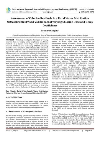
Available residual chlorine <0.2 mg/L for all the nodes at each reporting time step (1 hour) is collected for both Option-1 and Option-2 for all the chlorine doses (1 to 5 mg/L) and values are summarised and presented in tabularformatandcharts Itisobservedfromtheanalysis that a nos. of nodes require about 30 hours to get initial chlorine doseandWQAresultsforeachofthe last24hrs. (49 hrs. to 72 hrs.) are only presented in Table-2 and in theChart-1&Chart-2
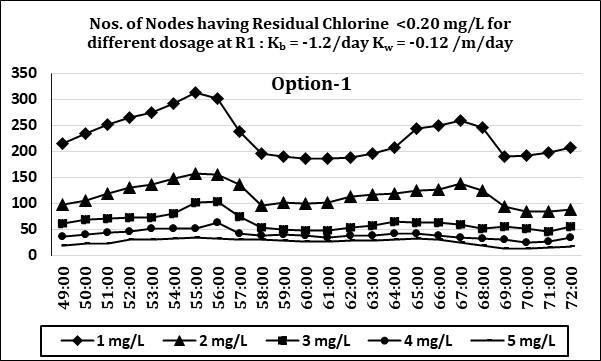
Chart-1 :ResidualChlorine<0.2mg/L–Option-1
International Research Journal of Engineering and Technology (IRJET) e-ISSN: 2395-0056
Volume: 12 Issue: 08 | Aug 2025 www.irjet.net p-ISSN: 2395-0072
The WDN, selected for this paper is a typical multi-village WDN having low demand and higher minimum diameter resultinginlowvelocityintheterminalpipelines.
For Option-1, even with a 5 mg/L chlorine dose, several nodes show available residual chlorine <0.2 mg/L throughout the day. With a 1 mg/L dose, about 50% of nodesshowavailableresidualchlorine<0.2mg/L.
ForOption-2,withlowervaluesofkbandkw,mostnodes have available residual chlorine >0.2 mg/L with a 2 mg/L or higher chlorine dose. However, with a 1 mg/L dose, somenodesstillhaveresidualchlorine<0.2mg/L.
Comparisonoftheresultswithhigherandlowervaluesof kb and kw with different dose of chlorine shows there are hugedifferencesinresidualchlorineatthefurthestnodes.
Tounderstandthecomplexbehaviourofchlorinedecayin aWDNseveralresearchersmadeseveralstudies
Ababuetal.(1)conductedbottletestexperimentstostudy the bulk decay of chlorine residual under varying initial chlorine doses. Their findings revealed that with an increase in the initial chlorine dose, the reaction rate constant for chlorine's bulk decay decreases, demonstratinganinverserelationshipbetweenthetwo.
Rossman et al. (13) suggests that applying a uniform wall decay constant for all pipes within a network may not be suitableforeverydistributionsystem.
Vasconcelos et al. (7) demonstrated that the chlorine reaction rate at the pipe wall is inversely proportional to the pipe diameter and may be constrained by the rate of chlorinemasstransfertothewall.
The first-order chlorine decay model assumes uniform bulk decay rate even with higher contact time. This assumption results in lower value of residual chlorine at the furthest point of a WDN having low velocity which
seemstobeincorrectandneedtobemodifiedasindicated inthestudy(1).
After analysing the result, it concludes that, for the selectedWDNwithlowervelocityoftheterminalpipes: a) it is the decay coefficients and travel time which playsthemajorroleratherthanthedose; b) assumption of uniform decay rates for all the pipes for all initial dose of chlorine may not be correct.
The above findings match with the studies done by the researcherssomeofwhicharementionedabove.
This study also implies that it is crucial to obtain reliable valuesofkb andkwtounderstandtheactualbehaviourofa WDNduringWQA
As both kb and kw vary widely and case dependent, it is always better to find out the chlorine residuals at several locations after application of chlorine at Headworks or Booster stations of a similar WDN to standardised the values of kb and kw applicable for all the WDN of similar nature.Thisprocessshallberepeatedthroughouttheyear forany changethat mayoccurduetochangein quality of water over time, temperature and other factors. Based on suchtestresultsoptimalvaluesofkb andkw maybefixed. For large complex WDN, sensors combined with remote telemetry, could enable continuous online calibration of network chlorine decay models, adapting to changing conditionsovertime.
The study emphasizes the critical role of WQA in maintainingsafeandpotablewaterinWDNs.Chlorination, while effective, faces challenges due to chlorine decay during transport. In rural WDNs having low demand coupled with provision of higher diameter of pipe due to regulatory reason results in lower velocity leading to insufficient residual chlorine at the farthest nodes. The researchdemonstratesthatdecaycoefficientssignificantly impact chlorine residuals Considering, an uniform decay ratesthroughoutthelengthoftheWDNwithlongertravel timesmayneedattention.
The findings highlight the need for site-specific determinationofbulk(kb)andwalldecay(kw)coefficients through field testing. Implementing systematic WQA and adjustingchlorinedosebasedonreal-timemonitoringcan optimize disinfection while minimizing excess chlorine use. Future studies should focus on developing improved decay models tailored to rural Indian water supply conditions to ensure consistent and safe potable water distribution.
International Research Journal of Engineering and Technology (IRJET) e-ISSN: 2395-0056
Volume: 12 Issue: 08 | Aug 2025 www.irjet.net p-ISSN: 2395-0072
[1] Ababu T. T, Tesfamariam Y. D, Gabriel C. B, and Stanley J. N. (2019). “A Mathematical Model for Variable Chlorine Decay Rates in Water Distribution Systems.” Modelling and Simulation in Engg Vol 2019, ArticleID5863905.
[2] Agboka K M, Alfred O. M, and Charles C. (2019). “Residual Chlorine Decay in Juja Water Distribution NetworkusingEPANETModel.”Int.J.ofEngg.andAdv. Tech. (IJEAT) ISSN: 2249-8958, Volume-9 Issue-1, October,2019,332-334.
[3] B Kowalska, D Kowalski, and Anna Musz (2006). “Chlorine decay in water distribution systems.” EnvironmentProtectionEngineering,Vol.32,2006,No. 2.
[4] CPHEEO. Manual on Water Supply and Treatment Systems (Drink from tap) Part A: Engineering - Planning, Design and Implementation. 4thEdition.Governmentof IndiaMinistryOfHousingandUrbanAffairs.December 2023.
[5]DenisN.,PhillimonT.O.,InnocentB.andBhagabaP.P. (2019). “Assessment of probable causes of chlorine decayin waterBOTSWANA.”ISSN1816-7950(Online) =WaterSAVol.45No.2April2019.
[6]Grayman, W.,S. Kshirsagar,M.Rivera-Sustacheand M. Ginsberg. (2012). "An Improved Water Distribution System Chlorine Decay Model Using EPANET MSX." Journal of Water Management Modeling R245-21. doi: 10.14796/JWMM.R245-21.
[7] John J. Vasconcelos, Lewis A. Rossman, Walter M. Grayman,Paul F.Boulos,andRobertM. Clark. (1997). “Kinetics of Chlorine Decay.” Article, AWWA – July 1997.
[8] Julius Caesar, Kwio-Tamale, and Charles Onyutha. (2024). “Influence of physical and water quality parameters on residual chlorine decay in water distributionnetwork.”Heliyon10(2024)e30892.
[9] L. Monteiro, J. Carneiro and Didia I. C. Covas. (2020) “Modelling chlorine wall decay in a full-scale water supply system.” URBAN WATER JOURNAL 2020, VOL. 17,NO.8,754–762.
[10] P. R. Bhave and R. Gupta. Analysis of Water Distribution Networks. Narosa Publishing, 2006, 388416.
[11] R. Gupta, S. Dhapade, S. Ganguly and P. R. Bhave. (2012). “Water quality based reliability analysis for water distribution networks.” ISH Journal of Hydraulic Engineering Vol. 18, No. 2, June 2012, 80–89.
[12]RoopaliV.GoyalandH.M.Patel. (2015). “Analysisof residual chlorine in simple drinking water distribution system with intermittent water supply.” Appl Water Sci (2015) 5:311–319 DOI 10.1007/s13201-014-0193-7.
[13] Rossman Lewis A., Robert M. Clark, Walter M. Grayman. (1994) “Modeling Chlorine Residuals in Drinking-Water Distribution Systems.” J. of Env. Engg., Vol. 120, No. 4, July/August, ASCE, ISSN 07339372/94/0004-0803.
[14] Rossman Lewis A. (2020). EPANET 2.2 User Manual. U.S.EnvironmentalProtectionAgency.
International Research Journal of Engineering and Technology (IRJET) e-ISSN: 2395-0056
Volume: 12 Issue: 08 | Aug 2025 www.irjet.net p-ISSN: 2395-0072
WaterDistributionNetworkData–NodeTable Node LPM Node LPM Node LPM Node LPM
J1 0.321 J51 0.643 J101 0.184 J151 1.908
J2 1.056 J52 0.367 J102 0.597 J152 1.060
J3 1.561 J53 0.826 J103 2.571 J153 1.749
J4 1.607 J54 1.377 J104 2.984 J154 1.060
J5 0.184 J55 0.872 J105 1.745 J155 2.755
J6 1.102 J56 0.826 J106 1.974 J156 1.484
J7 1.515 J57 1.791 J107 1.607 J157 3.126
J8 0.551 J58 0.689 J108 3.030 J158 1.590
J9 0.689 J59 1.148 J109 5.234 J159 2.225
J10 0.872 J60 1.515 J110 4.316 J160 1.007
J11 1.423 J61 0.459 J111 2.525 J161 2.914
J12 0.275 J62 0.643 J112 0.918 J162 1.855
J13 0.918 J63 0.551 J113 1.791 J163 1.643
J14 0.551 J64 0.230 J114 0.689 J164 1.272
J15 0.321 J65 0.826 J115 2.020 J165 1.537
J16 1.607 J66 0.275 J116 0.918 J166 1.113
J17 0.781 J67 0.643 J117 1.928 J167 1.855
J18 0.643 J68 0.184 J118 1.332 J168 0.954
J19 1.837 J69 0.459 J119 2.525 J169 1.484
J20 2.250 J70 0.643 J120 1.377 J170 0.477
J21 2.250 J71 0.505 J121 1.102 J171 0.742
J22 1.745 J72 0.230 J122 1.286 J172 1.960
J23 1.056 J73 1.423 J123 8.520 J173 0.477
J24 0.918 J74 0.275 J124 8.611 J174 0.742
J25 0.413 J75 1.332 J125 4.280 J175 1.272
J26 0.321 J76 0.275 J126 5.645 J176 0.795
J27 2.938 J77 0.597 J127 4.218 J177 2.066
J28 3.581 J78 0.184 J128 1.799 J178 0.636
J29 3.306 J79 0.459 J129 1.091 J179 0.848
J30 0.367 J80 1.469 J130 2.433 J180 1.749
J31 1.240 J81 0.275 J131 1.930 J181 1.325
J32 0.459 J82 0.230 J132 1.594 J182 1.378
J33 0.964 J83 0.781 J133 4.530 J183 1.378
J34 0.367 J84 0.459 J134 1.762 J184 0.795
J35 0.367 J85 1.056 J135 5.029 J185 2.861
J36 3.857 J86 0.367 J136 1.332 J186 2.172
J37 1.561 J87 0.321 J137 2.893 J187 1.166
J38 1.699 J88 0.964 J138 3.719 J188 2.967
J39 1.240 J89 0.413 J139 4.637 J189 1.088
J40 0.321 J90 0.918 J140 2.250 J190 1.323
J41 0.275 J91 0.321 J141 0.476 J191 0.501
J42 0.184 J92 0.643 J142 5.140 J192 1.422
J43 0.781 J93 0.735 J143 1.166 J193 2.505
J44 0.826 J94 0.964 J144 2.702 J194 1.055
J45 0.230 J95 0.321 J145 3.020 J195 0.835
J46 0.689 J96 0.551 J146 1.007 J196 1.626
J47 1.010 J97 0.643 J147 6.729 J197 0.791
J48 0.321 J98 0.964 J148 3.497 J198 0.395
J49 0.643 J99 0.321 J149 3.179 J199 1.934
J50 0.275 J100 0.689 J150 1.219 J200 0.703
Table – 3 : NodeData(Contd.)
WaterDistributionNetwork
J201 1.934 J251 0.483 J301 3.118 J351 0.864 J202 1.494 J252 1.318 J302 3.005 J352 0.376
J203 0.923 J253 0.439 J303 1.315 J353 0.563 J204 0.483 J254 0.527 J304
J354 0.451 J205 1.934 J255 1.099 J305
J355 0.714 J206 1.626 J256 1.186 J306
J356 3.419 J207 0.483 J257
J307
J357 3.381 J208 1.977 J258 1.230 J308 1.766 J358 3.306 J209 0.439 J259
J260
J218
J222
J266
J267
J268
J269
J270
J271
J272
J223 0.264 J273
J224 0.308 J274
J318
J321
J322
J324
J225 0.923 J275 0.571 J325
J367
J368
J369
J370
J371
J372
J373
J374
J375 0.150
J226 0.659 J276 0.879 J326 4.996 J376 1.465
J227 0.747 J277
J228 0.395 J278
J327
J328
J229 0.835 J279 0.308 J329
J230 4.878 J280
J330
J231 1.230 J281 0.747 J331
J232 0.264 J282 0.527 J332
J233 5.053 J283 0.835 J333
J234 4.394 J284
J334
J235 0.527 J285 1.099 J335
J236 0.703 J286 0.747 J336
J377
J378
J379 0.563
J380 0.751
J381
J382 0.563
J383
J384
J385 0.413
J386 0.601 J237
J287
J337
J238 1.186 J288 1.626 J338
J387
J388 0.601 J239
J240
J289
J290
J339
J340
J389
J390
J241 1.099 J291 0.483 J341 0.413 J391 0.413 J242 0.923 J292 0.703 J342 0.376 J392 0.263
J243 2.505 J293 1.670 J343 1.127 J393 0.601 J244 0.395 J294 0.659 J344 0.225 J394 0.451
J245 0.835 J295 1.977 J345 0.601 J395 0.488
J246 0.923 J296 0.264 J346 0.526 J396 0.714
J247 3.603 J297 0.766 J347 1.465 J397 0.488
J248 0.747 J298 3.145 J348 0.413 J398 0.751
J249 2.505 J299 5.109 J349 0.939 J399 0.451
J250 0.571 J300 3.381 J350 0.488 J400 0.751
International Research Journal of Engineering and Technology (IRJET) e-ISSN: 2395-0056
Volume: 12 Issue: 08 | Aug 2025 www.irjet.net p-ISSN: 2395-0072
WaterDistributionNetworkData–NodeTable
Node LPM Node LPM Node LPM Node LPM
J401 0.413 J423 3.531 J445 1.052 J467 0.601
J402 0.263 J424 0.751 J446 0.601 J468 1.352
J403 0.751 J425 1.089 J447 0.826 J469 1.803
J404 1.315 J426 0.789 J448 0.338 J470 0.639
J405 0.751 J427 1.052 J449 1.352 J471 5.710
J406 0.413 J428 0.413 J450 0.451 J472 1.615
J407 0.714 J429 0.826 J451 0.676 J473 0.488
J408 0.714 J430 0.751 J452 0.563 J474 0.601
J409 1.690 J431 0.676 J453 1.089 J475 4.283
J410 0.751 J432 4.508 J454 0.826 J476 1.766
J411 0.864 J433 4.095 J455 0.751 J477 3.193
J412 0.714 J434 3.231 J456 1.540 J478 1.615
J413 0.563 J435 0.639 J457 0.826 J479 0.188
J414 1.202 J436 0.676 J458 2.517 J480 0.225
J415 1.352 J437 0.639 J459 0.601 J481 1.202
J416 0.263 J438 0.789 J460 0.338 J482 0.789
J417 0.751 J439 0.301 J461 1.165 J483 1.202
J418 1.277 J440 1.277 J462 2.141 J484 0.376
J419 0.413 J441 0.714 J463 1.803 J485 1.352
J420 0.902 J442 1.089 J464 1.352 J486 0.601
J421 1.428 J443 0.751 J465 0.376 J422 0.563 J444 0.338 J466 1.916 Table – 4 : PipeData
P49 J51 J49
P50
Volume: 12 Issue: 08 | Aug 2025 www.irjet.net p-ISSN: 2395-0072
P101 J96 J94 15
P151 J150 J149 12
P102 J94 J92 15 80.4 P152 J149 J151 55
Table – 4 : PipeData(Contd.)
P103 J103 J36 145 112 P153 J152 J151 10 5 80.4
P104 J103 J104 150 112 P154 J151 J153 30 98.6
P105 J104 J105 100 80.4 P155 J154 J153 10 5 80.4
P106 J105 J106 100 80.4 P156 J153 J155 40 98.6
P107 J106 J73 125 80.4 P157 J155 J156 15 0
P108 J104 J107 85 112 P158 J155 J157 90 98.6
P109 J108 J107 95 112 P159 J158 J157 16 0 80.4
P110 J108 J109 250 98.6 P160 J157 J159 65
P112 J110 J111 145 98.6 P162 J159 J161 60 98.6
P113 J117 J116 105 80.4 P163 J161 J162 18 5 80.4
P114 J119 J118 150 80.4 P164 J161 J163 45 98.6
P115 J115 J113 100 80.4 P165 J164 J163 85 80.4
P116 J113 J112 105 80.4 P166 J164 J165 40 80.4
P117 J115 J114 80 80.4 P167 J165 J166 11 0 80.4
P118 J121 J120 20 80.4 P168 J163 J167 35 98.6
P119 J120 J119 140 80.4 P169 J167 J168 95 80.4
P120 J111 J122 105 80.4 P170 J167 J169 55 80.4
P121 J122 J121 45 80.4 P171 J171 J172 75 80.4
P122 J121 J117 60 80.4 P172 J179 J181 85 80.4
P123 J117 J115 55 80.4 P173 J180 J178 65 80.4
P124 J111 J123 35 98.6 P174 J177 J176 80 80.4
P125 J123 J124 365 80.4 P175 J173 J174 45 80.4
P126 J124 J125 90 80.4 P176 J174 J175 25 80.4
P127 J125 J126 270 80.4 P177 J175 J172 70 80.4
P128 J126 J127 205 80.4 P178 J172 J170 50 80.4
P129 J127 J128 150 80.4 P179 J169 J181 40 80.4
P130 J123 J137 75 80.4 P180 J180 J177 10 0 80.4
P131 J133 J132 100 80.4 P181 J177 J175 30 80.4
P132 J137 J136 150 80.4 P182 J181 J180 10 80.4
P133 J134 J135 110 80.4 P183 J188 J187 11 5 80.4
P135 J130 J129 65 80.4 P185 J186 J184 80 80.4
P134 J135 J133 150 80.4 P184 J183 J185 13 5 80.4
P136 J133 J131 40 80.4 P186 J169 J188 55 80.4
P137 J131 J130 85 80.4 P187 J188 J186 12 5 80.4
P139 J19 J138 150 225.4 P189 J186 J185 10 80.4
P138 J137 J135 105 80.4 P188 J185 J182 14 0 80.4
P140 J138 J139 270 225.4 P190 J141 J189 40 5 201.8
P141 J140 J139 255 225.4 P191 J190 J189 52 0 201.8
P143 J141 J142 225 112 P193 J191 J192
P142 J140 J141 370 225.4 P192 J190 J191 26 5 125.4
P144
J144
P146 J145 J144 195 80.4 P196
Volume: 12 Issue: 08 | Aug 2025 www.irjet.net
Table – 4 : PipeData(Contd.)
P301 J300 J299 325
P302 J301 J300 150 179.4 P352 J353 J355 15 80.4
P303 J306 J305 140 80.4 P353 J355 J333 20 80.4
P304 J302 J303 185 80.4 P354 J347 J349 30 80.4
P305 J306 J304 110 80.4 P355 J349 J351 45 80.4
P306 J304 J302 235 80.4 P356 J345 J347 50 80.4
P307 J301 J306 90 80.4 P357 J356 J329 235 98.6
P308 J307 J301 200 179.4 P358 J357 J356 245 98.6
P309 J309 J310 40 80.4 P359 J358 J357 225 98.6
P310 J319 J318 35 80.4 P360 J359 J358 240 98.6
P311 J313 J314 40 80.4 P361 J360 J359 60 98.6
P312 J314 J312 50 80.4 P362 J360 J361 110 80.4
P313 J317 J319 35 80.4 P363 J362 J360 20 98.6
P314 J308 J310 245 80.4 P364 J363 J362 65 80.4
P315 J310 J315 40 80.4 P365 J363 J364 295 80.4
P316 J311 J314 160 80.4 P366 J364 J370 55 80.4
P317 J315 J317 25 80.4 P367 J371 J372 80 80.4
P318 J317 J316 25 80.4 P368 J364 J372 60 80.4
P319 J314 J315 25 80.4 P369 J367 J368 100 80.4
P320 J319 J307 20 98.6 P370 J370 J369 65 80.4
P321 J320 J307 200 179.4 P371 J369 J368 40 80.4
P322 J321 J320 60 80.4 P372 J368 J366 50 80.4
P323 J322 J320 95 179.4 P373 J366 J365 215 80.4
P324 J323 J322 85 112 P374 J373 J362 20 80.4
P325 J323 J324 35 80.4 P375 J373 J383 45 80.4
P326 J324 J325 115 80.4 P376 J379 J378 80 80.4
P327 J326 J323 280 112 P377 J381 J380 105 80.4
P328 J326 J327 115 80.4 P378 J376 J374 100 80.4
P329 J328 J326 300 112 P379 J378 J377 105 80.4
P330 J329 J328 130 112 P380 J383 J381 95 80.4
P331 J330 J329 45 80.4 P381 J381 J378 30 80.4
P332 J330 J331 40 80.4 P382 J378 J376 85 80.4
P333 J332 J330 25 80.4 P383 J376 J375 20 80.4
P334 J333 J332 30 80.4 P384 J383 J382 80 80.4
P335 J334 J336 315 80.4 P385 J384 J373 45 80.4
P336 J339 J340 40 80.4 P386 J385 J384 55 80.4
P337 J338 J337 65 80.4 P387 J398 J397 65 80.4
P338 J338 J336 35 80.4 P388 J400 J399 60 80.4
P339 J333 J340 40 80.4 P389 J386 J387 85 80.4
P340 J340 J338 40 80.4 P390 J388 J387 30 80.4
P341 J336 J335
P342
P343 J342 J343 50 80.4 P393 J394 J396 20 80.4
P344 J349 J348
P345
P346
P347 J355 J354 60 80.4
P348
P350
– 4 : PipeData(Contd.)
L = Length of the
Diameter