Issuu

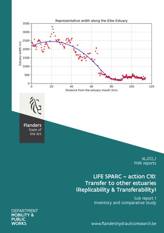
16_072_1 FHR reports

LIFE SPARC – action C10: Transfer to other estuaries (Replicability & Transferability) Sub report 1 Inventory and comparative study

www.flandershydraulicsresearch.be

LIFE SPARC – action C10: Transfer to other estuaries (Replicability & Transferability) Sub report 1 – Inventory and comparative study

Bi, Q.; Vanlede, J.; Mostaert, F.

The Life Sparc project has received funding from the LIFE Programme of the European Union

Cover figure © The Government of Flanders, Department of Mobility and Public Works, Flanders Hydraulics Research Legal notice Flanders Hydraulics Research is of the opinion that the information and positions in this report are substantiated by the available data and knowledge at the time of writing. The positions taken in this report are those of Flanders Hydraulics Research and do not reflect necessarily the opinion of the Government of Flanders or any of its institutions. Flanders Hydraulics Research nor any person or company acting on behalf of Flanders Hydraulics Research is responsible for any loss or damage arising from the use of the information in this report. Copyright and citation © The Government of Flanders, Department of Mobility and Public Works, Flanders Hydraulics Research 2021 D/2021/3241/222 This publication should be cited as follows: Bi, Q.; Vanlede, J.; Mostaert, F. (2021). LIFE SPARC – action C10: Transfer to other estuaries (Replicability & Transferability): Sub report 1 – Inventory and comparative study. Version 2.0. FHR Reports, 16_072_1. Flanders Hydraulics Research: Antwerp Reproduction of and reference to this publication is authorised provided the source is acknowledged correctly. Document identification Customer: Keywords (3-5): Knowledge domains:

ANB Ref.: WL2021R16_072_1 Estuary, Scheldt, Topo-bathymetry, Tidal range Hydraulics and sediment > Hydrodynamics > Tides > Literature and desktop study

Text (p.): Confidential:

40 ‫ ܈‬No

Author(s):

Bi, Q.

Appendices (p.): ‫ ܈‬Available online

Control Name Reviser(s):

Project leader:

Vanlede, J.

Signature

Getekend door:Joris Vanlede (Signature) Getekend op:2021-12-16 17:47:30 +01:0 Reden:Ik keur dit document goed

Getekend door:Joris Vanlede (Signature) Getekend op:2021-12-16 17:48:08 +01:0 Reden:Ik keur dit document goed

Approval Mostaert, F. Head of Division:

F-WL-PP10-2 Version 7 Valid as from 3/01/2017

For the Head of Division, absent Patrik Peeters, Engineer, in charge with leading the Division Flanders Hydraulics Research

Getekend door:Patrik Peeters (Signature) Getekend op:2021-10-19 16:12:24 +02:0 Reden:Ik keur dit document goed

LIFE SPARC – action C10: Transfer to other estuaries (Replicability & Transferability) Sub report 1 – Inventory and comparative study

Abstract The concept of combining Flood Control Areas (FCA) and Areas with a Controlled Reduced Tide (CRT) to give “Space to the River” is an original idea that has been developed, implemented and monitored in a pilot project in Flanders, Belgium. Through years of development, this nature-based solution is proved to be an effective approach of providing protection against flooding and improving resilience of the estuary ecosystem under the threat of climate change. One of the important goals in the LIFE-SPARC project is to perform knowledge transfer of the FCA/CRT method, including the design methodology, the expected effects and the monitoring plan with European partners. This report is aligned with the LIFE-SPARC project Action C10: Transfer to other estuaries (Replicability & Transferability). This action aims to assess the applicability of the core concept in other European Estuaries. In the LIFE-SPARC project, an idealised modelling approach is proposed as a tool for assessing the applicability for six European estuaries. This approach requires schematization of the geometry and the measures in each estuary, and only the important physical processes will be considered. As the first step of the comparative study, this report focuses on the schematization of estuary geometry. The necessary data consisting of the characteristics of each estuary has been collected and analysed. The representative geometry of each estuary is derived and will be used in the idealised modelling later.

Final version

WL2021R16_072_1

III

F-WL-PP10-2 Version 7 Valid as from 3/01/2017

LIFE SPARC – action C10: Transfer to other estuaries (Replicability & Transferability) Sub report 1 – Inventory and comparative study

Contents Abstract ............................................................................................................................................................ III Contents ............................................................................................................................................................ V List of tables..................................................................................................................................................... VII List of figures .................................................................................................................................................. VIII 1

Abbreviations............................................................................................................................................. 1

Introduction ............................................................................................................................................... 2 2.1

LIFE..................................................................................................................................................... 2

2.2

LIFE SPARC ......................................................................................................................................... 3

2.2.1

Project........................................................................................................................................ 3

2.2.2

Background ................................................................................................................................ 3

2.2.3

Objectives .................................................................................................................................. 3

2.3

Action C10: Transfer to other estuaries (Replicability & Transferability) ......................................... 4

2.3.1

CRT Technique ........................................................................................................................... 4

2.3.2

Applicability of FCA and CRT in other European estuaries ........................................................ 5

Methodology ............................................................................................................................................. 6 3.1

Idealised modelling of FCA and CRT in European estuaries. ............................................................. 6

3.2

Deriving the representative geometry .............................................................................................. 7

3.2.1

Definition of cross-sections ....................................................................................................... 8

3.2.2

Deriving morphological parameters and tidal characteristics................................................... 9

3.2.3

Representative width and bottom elevation ............................................................................ 9

3.2.4

Curve fitting ............................................................................................................................... 9

Data description ...................................................................................................................................... 11 4.1

Topo-bathymetry............................................................................................................................. 11

4.2

The tidal characteristics ................................................................................................................... 11

Scheldt estuary ........................................................................................................................................ 12 5.1

Introduction ..................................................................................................................................... 12

5.2

The representative geometry .......................................................................................................... 13

5.3

Tidal Range ...................................................................................................................................... 15

Elbe estuary ............................................................................................................................................. 16 6.1

Introduction ..................................................................................................................................... 16

6.2

The representative geometry .......................................................................................................... 17

Final version

WL2021R16_072_1

LIFE SPARC – action C10: Transfer to other estuaries (Replicability & Transferability) Sub report 1 – Inventory and comparative study

6.3 7

Tidal Range ...................................................................................................................................... 20

Weser estuary.......................................................................................................................................... 21 7.1

Introduction ..................................................................................................................................... 21

7.2

The representative geometry .......................................................................................................... 22

7.3

Tidal Range ...................................................................................................................................... 25

Humber estuary ....................................................................................................................................... 26 8.1

Introduction ..................................................................................................................................... 26

8.2

The representative geometry .......................................................................................................... 27

8.3

Tidal range ....................................................................................................................................... 29

Seine estuary ........................................................................................................................................... 30 9.1

Introduction ..................................................................................................................................... 30

9.2

The representative geometry .......................................................................................................... 31

9.3

Tidal Range ...................................................................................................................................... 33

Ems estuary ......................................................................................................................................... 34

10.1

Introduction ..................................................................................................................................... 34

10.2

The Representative geometry ......................................................................................................... 35

Conclusions .......................................................................................................................................... 37

References ....................................................................................................................................................... 38 Appendix: morphological parameters of the estuaries .................................................................................. A1 I. Scheldt ...................................................................................................................................................... A1 II. Elbe .......................................................................................................................................................... A3 III. Weser...................................................................................................................................................... A4 IV. Humber................................................................................................................................................... A6 V. Seine ........................................................................................................................................................ A7

WL2021R16_072_1

Final version

LIFE SPARC – action C10: Transfer to other estuaries (Replicability & Transferability) Sub report 1 – Inventory and comparative study

List of tables Table 1 – The spacing between the cross-section in the estuaries ................................................................... 8 Table 2 – The functions used in the curve fitting (x is the distance from the mouth) .................................... 10 Table 3 – Fitted parameters for the Scheldt estuary width ............................................................................ 13 Table 4 – Fitted parameters for the bottom elevation of the Scheldt estuary ............................................... 13 Table 5 – Fitted parameters for the Elbe estuary width ................................................................................. 17 Table 6 – Fitted parameters for the bottom elevation of the Elbe estuary .................................................... 18 Table 7 – Fitted parameters for the Weser estuary width .............................................................................. 23 Table 8 – Fitted parameters for the bottom elevation of the Weser estuary................................................. 23 Table 9 – Fitted parameters for the Humber estuary width ........................................................................... 27 Table 10 – Fitted parameters for the bottom elevation of the Humber estuary ............................................ 28 Table 11 – Fitted parameters for the Seine estuary width.............................................................................. 31 Table 12 – Fitted parameters for the bottom elevation of the Seine estuary ................................................ 32 Table 13 – Fitted parameters for the Seine estuary width.............................................................................. 35 Table 14 – Fitted parameters for the bottom elevation of the Seine estuary ................................................ 36

Final version

WL2021R16_072_1

VII

LIFE SPARC – action C10: Transfer to other estuaries (Replicability & Transferability) Sub report 1 – Inventory and comparative study

List of figures Figure 1 – Operational principle of a Flood Control Area (FCA) without (left panel) and with (middle and right panels) a Controlled Reduced Tide (CRT).................................................................................................. 4 Figure 2 – Width-averaged bed level relative to mean sea level at Vlissingen and the estuary width of the Scheldt in 2010 .................................................................................................................................................. 7 Figure 3 – An example of the cross-sections along the estuary (Seine) ............................................................ 8 Figure 4 – Map of the tidal part of the Scheldt River from Vlissingen to Ghent ............................................. 12 Figure 5 – Representative width along the Scheldt Estuary............................................................................ 14 Figure 6 – Representative bottom elevation along the Scheldt Estuary ......................................................... 14 Figure 7 – Water level at MHW and MLW and tidal range along the Scheldt estuary ................................... 15 Figure 8 – Overview of the Elbe estuary ......................................................................................................... 16 Figure 9 – Representative width along the Elbe Estuary................................................................................. 19 Figure 10 – Representative bottom elevation along the Elbe Estuary ............................................................ 19 Figure 11 – Water level at MHW and MLW and tidal range along the Elbe estuary ...................................... 20 Figure 12 – Overview of the Weser Estuary .................................................................................................... 21 Figure 13 – Representative width along the Weser Estuary ........................................................................... 24 Figure 14 – Representative bottom elevation along the Weser Estuary ........................................................ 24 Figure 15 – Water level at MHW and MLW and tidal range along the Weser Estuary ................................... 25 Figure 16 – Overview of the Humber Estuary ................................................................................................. 26 Figure 17 – Representative width along the Humber Estuary ........................................................................ 28 Figure 18 – Representative bottom elevation along the Humber Estuary ..................................................... 29 Figure 19 – Water level at MHW and MLW and tidal range along the Humber Estuary ................................ 29 Figure 20 – Overview of the Seine estuary...................................................................................................... 30 Figure 21 – Representative width along the Seine Estuary ............................................................................. 32 Figure 22 – Representative bottom elevation along the Seine Estuary .......................................................... 33 Figure 23 – Water level at MHW and MLW and tidal range along the Seine Estuary..................................... 33 Figure 24 – The overview of the Ems estuary ................................................................................................. 34 Figure 25 – Representative width along the Ems Estuary ............................................................................... 36 Figure 26 – Representative bottom elevation along the Ems Estuary ............................................................ 36 Figure 27 – Width along the Scheldt Estuary .................................................................................................. A1 Figure 28 – Wet section area along the Scheldt Estuary ................................................................................. A2 Figure 29 – Cross-sectionally averaged water depth along the Scheldt Estuary ............................................ A2 Figure 30 – Width along the Elbe Estuary ....................................................................................................... A3 Figure 31 – Wet section area along the Elbe Estuary ...................................................................................... A3

VIII

WL2021R16_072_1

Final version

LIFE SPARC – action C10: Transfer to other estuaries (Replicability & Transferability) Sub report 1 – Inventory and comparative study

Figure 32 – Cross-sectionally averaged water depth along the Elbe Estuary ................................................. A4 Figure 33 – Width along the Weser Estuary .................................................................................................... A4 Figure 34 – Wet section area along the Weser Estuary .................................................................................. A5 Figure 35 – Cross-sectionally averaged water depth along the Weser Estuary .............................................. A5 Figure 36 – Width along the Humber Estuary ................................................................................................. A6 Figure 37 – Wet section area along the Humber Estuary ............................................................................... A6 Figure 38 – Cross-sectionally averaged water depth along the Humber Estuary ........................................... A7 Figure 39 – Width along the Seine Estuary ..................................................................................................... A7 Figure 40 – Wet section area along the Seine Estuary .................................................................................... A8 Figure 41 – Cross-sectionally averaged water depth along the Seine Estuary................................................ A8

Final version

WL2021R16_072_1

LIFE SPARC – action C10: Transfer to other estuaries (Replicability & Transferability) Sub report 1 – Inventory and comparative study

1 Abbreviations Abbreviation

Meaning

CRT

Controlled Reduced Tide

FCA

Flood Control Area

MLW

Mean Low Water

MHW

Mean High Water

Final version

WL2021R16_072_1

LIFE SPARC – action C10: Transfer to other estuaries (Replicability & Transferability) Sub report 1 – Inventory and comparative study

2 Introduction 2.1 LIFE The LIFE programme is the EU’s funding instrument for the environment and climate action. The general objective of LIFE is to contribute to the implementation, updating and development of EU environmental and climate policy and legislation by co-financing projects with European added value. The European Commission (DG Environment and DG Climate Action) manages the LIFE programme. The LIFE 2014-2020 Regulation (EC) No 1293/2013 was published in the Official Journal L 347/185 of 20 December 2013. The Regulation establishes the Environment and Climate Action sub-programmes of the LIFE Programme. The ‘Environment’ strand of the new programme covers three priority areas: environment and resource efficiency; nature and biodiversity; and environmental governance and information. The ‘Climate Action’ strand covers climate change mitigation; climate change adaptation; and climate governance and information. This project falls under Climate Change Adaptation. From the EU regulation that establishes the LIFE programme, article 15: Specific objectives for the priority area Climate Change Adaptation With a view to contributing to supporting efforts leading to increased resilience to climate change, the priority area Climate Change Adaptation shall in particular have the following specific objectives: (a) to contribute to the development and implementation of Union policy on climate change adaptation, including mainstreaming across policy areas, in particular by developing, testing and demonstrating policy or management approaches, best practices and solutions for climate change adaptation, including, where appropriate, ecosystem-based approaches; (b) to improve the knowledge base for the development, assessment, monitoring, evaluation and implementation of effective climate change adaptation actions and measures, prioritising, where appropriate, those applying an ecosystem-based approach, and to enhance the capacity to apply that knowledge in practice; (c) to facilitate the development and implementation of integrated approaches, such as for climate change adaptation strategies and action plans, at local, regional or national level, prioritising, where appropriate, ecosystem-based approaches; (d) to contribute to the development and demonstration of innovative climate change adaptation technologies, systems, methods and instruments that are suitable for being replicated, transferred or mainstreamed.

WL2021R16_072_1

Final version

LIFE SPARC – action C10: Transfer to other estuaries (Replicability & Transferability) Sub report 1 – Inventory and comparative study

2.2 LIFE SPARC 2.2.1

Project

LIFE SPARC is a project under the LIFE programme (project number LIFE16 CCA/BE/000107). SPARC is the acronym for “Space for Adapting the River Scheldt to Climate Change”. The project runs from 01/09/2017 till 31/08/2022. The project partners are: • • • • • 2.2.2

Agentschap voor Natuur en Bos (coordinating beneficiary) Eigen Vermogen Flanders Hydraulics Flanders Hydraulics Research Regionaal Landschap Schelde-Durme Waterwegen en Zeekanaal NV Background

Climate change entails raising sea levels and increasing risks from extreme weather phenomena. The Scheldt estuary (Belgium) is highly vulnerable to flooding because of its open connection to the sea, its funnel-shape and surrounding low-lying land, especially when high tides coincide with heavy rainfall. The Scheldt is laden with sediment, so tidal marshes are systematically rising along with high waters. Consequently, the transition to the waterway is becoming steeper (squeeze). The steep tidal marshes risk being eroded. As a result, protected freshwater mud flat and tidal marsh habitats, which are rare in Europe, are disappearing. These habitats also provide important ecosystem services. Financial damage from flooding in the Scheldt estuary can exceed €50 million on an annual basis. In the Belgian part of the estuary (the tide-affected area) there are approximately 720 000 inhabitants and 10 000 businesses situated in low-lying areas at potential risk of flooding. In the port of Antwerp, where economic activity is concentrated, the consequences of a flood could be disastrous. Serious flooding would also affect inland waterways. 2.2.3

Objectives

The LIFE SPARC project proposes measures to make the Scheldt estuary and its highly urbanised area more resilient to climate change. In practice, this means providing much greater protection against flooding by creating open space for water and developing a robust estuary ecosystem. More specifically, the project has the following goals: 1. Reduce flood risk using nature-based solutions appropriate to tidal rivers, in line with the EU Floods Directive, such as the construction of flood areas that can safely fill with water during flood events, thereby decreasing water levels on the river and reducing the risk of flooding in urban areas; 2. Restore habitats to make the ecosystem more resilient to the effects of climate change, and enabling tidal mud flats and freshwater tidal marshes to develop in line with the Habitats Directive. The aim is for the restored sites to form a network, to improve the implementation of the Habitats and Birds directives and to act as green infrastructure ('corridors') to give species greater opportunity for movement; 3. Reinforcing public support, by actively engaging stakeholders and the general public, and sharing knowledge. Opportunities in the field of recreation and tourism will also be taken to boost the local economy; and 4. Demonstrating the transferability and replicability of new techniques for nature-based solutions appropriate to tidal rivers.

Final version

WL2021R16_072_1

LIFE SPARC – action C10: Transfer to other estuaries (Replicability & Transferability) Sub report 1 – Inventory and comparative study

2.3 Action C10: Transfer to other estuaries (Replicability & Transferability) The core concept of combining Flood Control Areas (FCA) and Areas with a Controlled Reduced Tide (CRT) to give “Space to the River” is an original idea that has been developed, implemented and monitored in a pilot project in Flanders, Belgium. The experience gained at the pilot site Lippenbroek (a CRT studied during the LIFE project MARS) combined with the development of 8 additional realizations during this project (actions C1- C8), complemented with additional knowledge gained in this action will be used to assess the applicability of the core concept in other European Estuaries. 2.3.1

CRT Technique

One of the measures in the Sigmaplan is to build a set of Flood Control Areas (FCAs). To this end, specific polders along the tidal river Scheldt are selected which have an elevation below mean high tide level. As a first construction step, a sufficiently high ring dike surrounding the polder needs to be built. Secondly, the existing levee between the polder and the river needs to be lowered, in order to create an overflow dike. During storm surges, water can overtop the overflow dike and be stored in the FCA, thus damping the tidal wave in the river and mitigating the flooding of nearby valuable areas. To drain the water from the FCA when the water level in the river is sufficiently low again, outlet sluices are included within the overflow dike (Error! Reference source not found., left). The corresponding culverts are equipped with flap gates on the river side. On average, such a FCA is flooded once or twice a year. An FCA-CRT is a variant of an FCA. It combines the safety role of a flood area with the restoration of rare tidal nature. Waterflows into and out of an FCA-CRT twice a day to the rhythm of the tides. The area is flooded at each high tide. A limited amount of waterflows in through the inlet sluice. In this way the tide is "reduced". When the tide ebbs, the water flows back into the river through the outlet sluice. The natural action of a tidal river is thus mimicked. The area effectively becomes part of the Scheldt ecosystem and a system of tidal marshes can develop. The CRT principle was developed by Professor Patrick Meire (University of Antwerp).

Figure 1 – Operational principle of a Flood Control Area (FCA) without (left panel) and with (middle and right panels) a Controlled Reduced Tide (CRT) (De Mulder et al., 2013)

The CRT technique is often unknown in the other EU member states but can also be used in other estuaries, especially under the following conditions: • • • • •

Available space is very limited, which means maximum storage capacity is required when the peak of the storm surge hits. The relative altitude of adjacent land is unfavourable in relation to the river, which prevents formation of proper mudflats - tidal marshes in case of depoldering. The embankment alongside the river needs to be retained and kept accessible. Large tidal fluctuations are undesirable in floodplains. Large depoldering operations are undesirable because the fairway is left without sufficient water at times

WL2021R16_072_1

Final version

LIFE SPARC – action C10: Transfer to other estuaries (Replicability & Transferability) Sub report 1 – Inventory and comparative study

For the CRT system to function properly, a carefully dimensioned culvert construction with combined inlet and outfall has to be placed at a specific height within the tidal window. This is the only way to secure an appropriate neap-spring tidal variation, which is crucial for the development of mudflats and tidal marshes in the area. 2.3.2

Applicability of FCA and CRT in other European estuaries

In order to perform knowledge transfer of the FCA/CRT method, the design methodology, the expected effects and the monitoring plan will be shared with European partners. In a series of workshops, we aim to perform a quickscan of the applicability of FCA and CRT in other European estuaries to obtain protection against flooding in combination with nature development. Experience in Flanders has shown that it is possible to combine the concept of a flood control area (FCA) with nature development and the functions of intertidal areas, by use of simple culvert constructions to introduce a controlled reduced tide (CRT). The term “Quickscan” is chosen to differentiate the work proposed in action C 10 with a complete design, which would take much longer to complete. With this action we want to show the applicability of the CRT concept (in terms of safety against flooding and nature development) in other European estuaries, in order to start a true discussion on transferability of the CRT technology. Letters of support were received from following partners Estuary Ems (Nederland) en Schelde Ems (Duitsland) Weser (Duitsland) Elbe (Duitsland) Seine (France) Humber (UK)

Institute Rijkswaterstaat - WVL BAW NLWKN - Niedersächsische Landesbetrieb für Wasserwirtschaft, Küsten- und Naturschutz HPA Groupement d'Intérêt Public Seine-Aval Environment Agency

Contact Herman Mulder Holger Rahlf Dr. Wilfried Heiber Dr. Maik Bohne Nicolas Bacq Philip Winn / Susan Manson

The workshops are organized in Antwerp in order to keep the costs of organizing the workshops as low as possible. This report is a deliverable under action C10, and aims for an inventory and comparative study of the estuaries mentioned above.

Final version

WL2021R16_072_1

LIFE SPARC – action C10: Transfer to other estuaries (Replicability & Transferability) Sub report 1 – Inventory and comparative study

3 Methodology 3.1 Idealised modelling of FCA and CRT in European estuaries. The estuaries in the Western Europe combine busy crossroads of transport routes with valuable ecological areas. They usually host important cities and ports, which are of significant importance for economics, while they also provide protected habitats for numerous species of fish, birds and sea mammals. However, these estuaries are under constant threat and subject to environmental pressures, which might impact the functioning of estuaries (Kaptein et al., 2020). For addressing the challenges and threats faced by the estuaries, the implementation of innovative management and engineering measures, e.g. FCA and CRT, is required. For studying the effect of FCA and CRT on tidal wave propagation, high water during storm conditions in particular, we can apply an idealized modelling approach. The idealised modelling approach consists of the following aspects: •

•

The schematization of the complex geometry and bathymetry. In nature, estuaries often have a complex geometry, with converging width towards a meandering tidal river upstream. But in general, this complex geometry can be simplified while maintaining important properties like the characteristics of tidal propagation. The schematization of physical processes. Usually there are many physical processes happening in a estuarine system, e.g. (tidal) wave propagation, transport of suspended matter, salinity mixing, ecological processes. In idealised modelling, depending on the research focus, only the important processes are included in the model. The schematization of the measures. The measures, e.g. FCA and CRT, consists of sophisticated hydraulic structures, and an area of land adjacent to them that can experience flooding during periods of high water. Both the structure and the area of the land have to be schematized in an idealised model. However, the dynamics between the main channel and the FCA and CRT will be kept for proper modelling the effects of these measures.

The purpose of using idealised modelling approach is to have a quick assessing tool to study the effects of implementing FCA and CRT in many other European estuaries, and check if they will achieve similar positive influences to the safety of the region and to the ecological system. The location of the flood control areas along the estuary, their surface area (and thus retention capacity) and the hydraulic characteristics (height of the overflowing dike; height and dimensions of the culverts) can all be varied. These different combinations will naturally cause different effects to the system. So the question of effect quantification becomes a problem with a lot of degrees of freedom. Li et al (2016) have shown that simple 1D models can be used as a quick assessment method. They tested 512 combinations of 9 retention basins in the Ems using an idealized one-dimensional linear model. Recently, the influence of retention basins has been systematically studied using more simplified crosssectionally averaged models (Alebregtse et al., 2013; Alebregtse and De Swart, 2014; Roos and Schuttelaars, 2015). This existing body of work shows the important effect of the location of the areas on their effect on tidal wave propagation in the estuary. In contrast to this existing body of work (that uses simplified equations), we propose to use idealised models built in a shallow water solver, including the culvert function. This way, the specific hydraulic characteristics of FCA and CRT can be represented more accurately compared to the more analytical approach. In order to make optimal use of existing data on the geometry and bathymetry of the estuaries, we propose to characterize the geometry in terms of the hydro-geomorphological characteristics that were quantified in the TIDE project (Vandenbruwaene et al, 2013):

WL2021R16_072_1

Final version

LIFE SPARC – action C10: Transfer to other estuaries (Replicability & Transferability) Sub report 1 – Inventory and comparative study

• • • •

Width along the estuary Wet section along the estuary Mean high/low water level along the eatery Convergence length

These are reported for the Scheldt, Elbe, Weser and Humber in the TIDE project (Vandenbruwaene et al, 2013). Recently, the similar data were also reported for the Seine (Vandenbruwaene et al., 2017). The Ems data was provided by Dijkstra et al. (2019b). For the idealised modelling of physical process, we focus on the hydrodynamics only, investigating the effects of FAC and CRT with different combinations of characteristics to the hydrodynamics in different estuaries.

3.2 Deriving the representative geometry The geometry of the estuary could change dramatically along the main channel, starting much wider in the mouth region and then converging to a much narrower tidal river towards upstream. The bottom of the estuary usually varies in two directions, along the thalweg of the channel (deeper in the estuary mouth and shallower when it reaches further upstream), and across (deeper in the middle of the channel and shallower when it is close to the banks). When deriving the geometry for building an idealised model, it is important to choose an appropriate method to perform schematization. In the study of Dijkstra et al. (2019a), a schematized Scheldt model is created using the observed morphological data. The Scheldt Estuary is schematized as a funnel-shaped single channel from the mouth at Vlissingen to the tidal weir and locks at Ghent. Tidal propagation into the tributaries is not explicitly taken into account.

Figure 2 – Width-averaged bed level relative to mean sea level at Vlissingen and the estuary width of the Scheldt in 2010 (Dijkstra et al. 2019a)

The width (W) of the Scheldt in the model is obtained by the average of the width measured at the surface at high and low water and is fitted by a smooth function. The width-averaged bed level (B) of the Scheldt is derived by subtracting the cross-sectionally averaged water depth from the mean water level at high and low water, respectively, and then taking the average of the two. The resulting bottom elevation is fitted using a smooth polynomial function. A similar methodology is applied for schematizing the geometry for all the 6 estuaries in this study. The morphological parameters at high and low water, e.g. the estuarine width, the cross-sectionally averaged water depth, are considered essential. Moreover, the mean high water (MHW) level and mean low water (MLW) level are also required.

Final version

WL2021R16_072_1

LIFE SPARC – action C10: Transfer to other estuaries (Replicability & Transferability) Sub report 1 – Inventory and comparative study

3.2.1

Definition of cross-sections

In order to capture the spatial variation of the characteristics along each estuary, it is necessary to define regularly spaced cross-sections starting from the estuary mouth all the way to the upstream boundary. Then the morphological parameters, e.g. estuarine width and cross-sectionally averaged water depth can be computed at these cross-sections, as well as other variables that represent the tidal characteristics. But before defining the cross-sections, a consistent definition of the estuary mouth for all the estuaries is needed. Different criteria (shape, tidal influence, river influence, geology, salinity) can be used to define the mouth of an estuary (e.g., Savenije, 2005). In this study, the estuary mouth is defined based on the width change: once the width change at MHW level is below a certain threshold value, at that location the mouth area stops and the estuary starts. This definition is necessary for studying the effect of estuary funneling on the tidal amplification (Vandenbruwaene et al. 2013), which is also the focus in the project.

Figure 3 – An example of the cross-sections along the estuary (Seine)

An example of the defined cross-sections for the Seine is shown in Figure 3Error! Reference source not found.. The regular distances between the cross-sections used in all the estuaries are listed in Table 1. Table 1 – The spacing between the cross-section in the estuaries

Name of the estuary Distance between cross-sections Scheldt

200 m

Elbe

250 m

Weser

500 m

Humber

250 m

Seine

500 m

Ems

5000 m

Then the defined cross-sections are indexed by their distance to the estuary mouth.

WL2021R16_072_1

Final version

LIFE SPARC – action C10: Transfer to other estuaries (Replicability & Transferability) Sub report 1 – Inventory and comparative study

3.2.2

Deriving morphological parameters and tidal characteristics

The following morphological parameters are derived at the cross-sections of each estuary. •

The estuarine width

The topo-bathymetry data was processed with the MikeGIS software, which can automatically derive the width at any reference level Vandenbruwaene et al. (2013 and 2018). In this case, the reference level can be the mean high water level and mean low water level, respectively. In principle, the estuary width is measured at each cross-section by computing the distance between the two end points on the cross-section. •

The cross-sectionally averaged water depth

The cross-sectionally averaged water depth can be obtained by dividing the wet-section area by the estuarine width. The wet-section area is defined as the cross-sectional area at the reference water level (MHW and MLW in this case). The cross-sectional area is another output given by the MikeGIS software when processing the topo-bathymetry data (Vandenbruwaene et al., 2013 and 2018). It is computed by integrating the water depth at the sampled points along each cross-section during mean high water and mean low water, respectively. The tidal characteristics, e.g. mean high water level and mean low water level, are usually measured at stations in the estuary. They are obtained by averaging the water levels during a specific period, e.g. high water and low water. The monitoring stations are usually not evenly spaced. In this case, the data points have to be interpolated at the defined cross-sections. Then it is possible to calculate the bottom elevation by subtracting the cross-sectionally averaged water depth from the mean water levels at each cross-section. 3.2.3

Representative width and bottom elevation

The geometry data from Vandenbruwaene et al. (2013 and 2018) and Dijkstra et al. (2019b) is used to compute the representative width and bottom elevation for schematization of the estuaries. More specifically,

𝐵𝐵𝑟𝑟𝑟𝑟𝑟𝑟

𝑊𝑊𝑀𝑀𝑀𝑀𝑀𝑀 + 𝑊𝑊𝑀𝑀𝑀𝑀𝑀𝑀 2 1 𝐴𝐴𝑀𝑀𝑀𝑀𝑀𝑀 𝐴𝐴𝑀𝑀𝑀𝑀𝑀𝑀 = ��𝑊𝑊𝑊𝑊𝑀𝑀𝑀𝑀𝑊𝑊 − � + �𝑊𝑊𝑊𝑊𝑀𝑀𝑀𝑀𝑀𝑀 − �� 𝑊𝑊𝑀𝑀𝑀𝑀𝑀𝑀 𝑊𝑊𝑀𝑀𝐿𝐿𝑊𝑊 2 𝑊𝑊𝑟𝑟𝑟𝑟𝑟𝑟 =

(6)

(7)

in which, 𝑊𝑊𝑟𝑟𝑟𝑟𝑟𝑟 is the representative estuary width, 𝑊𝑊𝑀𝑀𝑀𝑀𝑀𝑀 is the estuary width at mean high water level, 𝑊𝑊𝑀𝑀𝑀𝑀𝑀𝑀 is the estuary width at mean low water level, 𝐵𝐵𝑟𝑟𝑟𝑟𝑟𝑟 is the representative estuary bottom elevation, 𝑊𝑊𝑊𝑊𝑀𝑀𝑀𝑀𝑀𝑀 is the mean high water level, 𝑊𝑊𝑊𝑊𝑀𝑀𝑀𝑀𝑀𝑀 is the mean low water level, 𝐴𝐴𝑀𝑀𝑀𝑀𝑀𝑀 is the wet section area at mean high water level, and 𝐴𝐴𝑀𝑀𝑀𝑀𝑀𝑀 is the wet section area at mean low water level.

The collected datasets of the estuaries have different reference level since they located in different countries. In this study, they all have been converted into the mean sea level (MSL). 3.2.4

Curve fitting

For getting a smooth outline for the schematized geometry, curve (data) fitting has to be performed. The same procedure should be done with the derived bottom elevation as well. An overview of the functions that can be used in curve fitting are listed in Table 2. More details can be found in Dijkstra (2017).

Final version

WL2021R16_072_1

LIFE SPARC – action C10: Transfer to other estuaries (Replicability & Transferability) Sub report 1 – Inventory and comparative study

Table 2 – The functions used in the curve fitting (x is the distance from the mouth)

Function

Expression

Exponential

𝑓𝑓 = 𝐶𝐶0 ∙ 𝑒𝑒 −𝑥𝑥/𝐿𝐿𝑐𝑐

ExpRationalFunc

𝑓𝑓 = 1000 ∙ 𝑒𝑒 polyval(𝐶𝐶1 ,𝑥𝑥)/polyval(𝐶𝐶2 ,𝑥𝑥) 𝑓𝑓 = 𝐶𝐶0 + 𝐶𝐶1 ∙ tanh �

HyperbolicTangent Polynomial

PolynomialLinear

Remarks

𝑥𝑥 − 𝑥𝑥𝑐𝑐 � 𝑥𝑥𝑙𝑙

𝑓𝑓 = polyval(𝐶𝐶, 𝑥𝑥) �

polyval(𝐶𝐶, 𝑥𝑥) 𝑖𝑖𝑖𝑖 𝑥𝑥 < 𝑋𝑋𝐿𝐿 polyval(𝐶𝐶, 𝑋𝑋𝐿𝐿 ) + 𝑝𝑝𝑝𝑝𝑝𝑝𝑝𝑝𝑝𝑝𝑝𝑝𝑝𝑝(𝐶𝐶, 𝑋𝑋𝐿𝐿 )(𝑥𝑥 − 𝑋𝑋𝐿𝐿 ) 𝑖𝑖𝑖𝑖 𝑥𝑥 > 𝑋𝑋𝐿𝐿

𝐶𝐶0 and 𝐿𝐿𝑐𝑐 are the fitted parameters 𝐶𝐶1 and 𝐶𝐶2 contain polynomial coefficients 𝐶𝐶0 , 𝐶𝐶1 , 𝑥𝑥𝑐𝑐 and 𝑥𝑥𝑙𝑙 are fitted parameters 𝐶𝐶 contains polynomial coefficients 𝐶𝐶 contains polynomial coefficients, 𝑋𝑋𝐿𝐿 is the connection point

It is worthwhile to mention that in the exponential function, fitted parameter 𝐿𝐿𝑐𝑐 usually refers to the width convergence length, and 𝐶𝐶0 is the width at the estuary mouth. The tidal penetration in an estuary is influenced by several factors, with the most important factors being the funnel shape of the estuary, leading to an amplification of the tidal range, and the friction within the estuary, leading to a decrease in tidal range. The estuarine convergence can be described as in (Vandenbruwaene et al., 2013) by the width convergence length 𝐿𝐿𝑐𝑐 .

In what follows, the exponential function, exponential rational function, hyperbolic tangent function and their combinations are often used in curve fitting of the geometry, while the polynomial and polynomial linear function are used in curve fitting of the bathymetry.

WL2021R16_072_1

Final version

LIFE SPARC – action C10: Transfer to other estuaries (Replicability & Transferability) Sub report 1 – Inventory and comparative study

4 Data description For obtaining the representative geometry and bathymetry of each estuary, the topo-bathymetry and tidal characteristics were collected. The topo-bathymetry data and tidal characteristics were directly measured in the estuaries and other important morphological parameters, e.g. the estuary width, the thalweg depth, wet-section area can be derived from them. From the results of the TIDE project (Vandenbruwaene et al., 2013 and 2018), the processed topo-bathymetry data and tidal characteristics were available for the Scheldt, Elbe, Weser, Humber and Seine. The morphological parameters, such as estuarine width and cross-sectionally averaged depth along these estuaries have already been derived. For the Ems, the estuarine width and depth is taken from Dijkstra et al. (2019b). These datasets and how they were processed are described in the following sections.

4.1 Topo-bathymetry The topo-bathymetric data of an estuary represent the elevation of the subtidal, intertidal and supratidal areas. In general, the bathymetric data (based on multibeam or single-beam measurements) cover the subtidal and lower intertidal parts of the estuary, while the topographic datasets (based on LIDAR data) cover the higher parts of the intertidal areas and tidal marsh areas (supratidal). For the Scheldt and Elbe topo-bathymetric grids were directly available, respectively for the years 2001 and 2006. The Scheldt grid has a resolution varying between 5 x 5 m and 20 x 20 m, the Elbe grid has a resolution of 10 x 10 m. For the Weser and Humber, point datasets were delivered and interpolated to grids of those areas. The input datasets were respectively from 2009 and 2005 for the Weser and Humber, and interpolation grids were created with a resolution of respectively 20 x 20 m and 10 x 10 m. Seine topo-bathymetric data were provided for the 2010 and it has a 5 x 5 m topo-bathymetric ESRI raster ranging from the Seine mouth up to Pont-de-l’Arche (Vandenbruwaene et al., 2013). For the Ems, The original bathymetry data of Ems was owned by the WSA Emden. In the study of Dijkstra et al. (2019b), the original data was processed in order to derive the representative geometry and bathymetry. The width of the estuary is estimated from satellite images and the shallow areas and the Dollard bay have been ignored (Dijkstra et al. 2019b). Channel depth data for the year 2005 were obtained from Wasserstraßen- und Schifffahrtsamt Emden Emden and were presented earlier by de Jonge et al. (2014). The processed data with the morphological parameters from Dijkstra et al. (2019b) is provided and used in this study for deriving the idealized geometry and bathymetry for the Ems. The morphological parameters of the estuaries derived from the topo-bathymetric data are shown in the Appendix: morphological parameters of the estuaries.

4.2 The tidal characteristics For each estuary the main water level parameters (mean high water level = MHW, mean low water level = MLW) were delivered for a number of stations along the estuary. A 10-yearly average (2001-2010) was therefore used for the Scheldt, Elbe and Weser. For the Humber data from the period 2005-2010 were used. For the Seine, data from the period 2007-2010 were used. The detailed measurements of water levels were not required for the Ems, since the processed data was provided, which was the measured amplitudes and phases of M2 and M4 tides in 2005 from the study of Dijkstra et al. (2019b). The difference between mean high water (MHW) and mean low water (MLW) gives the tidal range.

Final version

WL2021R16_072_1

LIFE SPARC – action C10: Transfer to other estuaries (Replicability & Transferability) Sub report 1 – Inventory and comparative study

5 Scheldt estuary 5.1 Introduction The Scheldt estuary is defined as the part of the river basin under tidal influence. It is a well-mixed estuary opening to the southern North Sea and extends 160 km in length from the mouth at Vlissingen to Ghent, where sluices stop the tidal wave in the Upper Scheldt. The tidal wave also penetrates most of the upstream areas, entering the major tributaries Rupel and Durme, resulting in approximately 235 km of tidal river in the estuary. In the Scheldt estuary at Vlissingen, the tidal amplitude is about four meters. Further inland, the tidal range increases. The further upstream, the narrower the riverbed and the more the incoming floodwater is pushed up. Near Hamme, where the Durme flows into the Scheldt, the river reaches its highest water level. The locks around Ghent blocks the tide completely and ensure that the river further upstream is no longer influenced by the tide (Vlaams-Nederlandse Schelde Commissie, 2015).

Figure 4 – Map of the tidal part of the Scheldt River from Vlissingen to Ghent (Dijkstra et al., 2019a)

The Scheldt estuary is one of the youngest and most natural estuaries in Western Europe. It consists of an approximately 60 km long fresh water tidal zone stretching from near the mouth of Rupelmonde to Ghent, representing one of the largest freshwater tidal areas in Western Europe. It has a salinity mixing zone between Rupelmonde and Vlissingen/Breskens. The subtidal delta, seaward of Vlissingen forms the transition between the Western Scheldt and the North Sea. (Fettweis et al., 1998; Kuijper et al., 2004; Meire et al., 2005; van Kessel et al., 2011). The Scheldt estuary can be divided into two major parts, the Sea Scheldt (Zeeschelde) (length 105 km), which is the Belgian part from Ghent to the Dutch/Belgian boarder, and the Western Scheldt (Westerschelde) (length 58 km), which is the Dutch part covering the middle and lower estuary. The Sea Scheldt consist of one single ebb/flood channel and has a total surface area of 44 km2. Mudflats and marshes in this area are relatively small and approximately account for 28% of the total surface. The Sea Scheldt hosts one of the largest harbours in Europe – the Port of Antwerp. Therefore, human activities are very important in this region and industrial developments are concentrated along the riverbanks. The intertidal zone is often missing or very narrow. The estuary is almost completely canalized upstream of Dendermonde (Hoffmann & Meire, 1997).

WL2021R16_072_1

Final version

LIFE SPARC – action C10: Transfer to other estuaries (Replicability & Transferability) Sub report 1 – Inventory and comparative study

The Western Scheldt is a well-mixed region. Due to the influences of tidal waves and land changes, the Western Scheldt has a complex and dynamic morphology. The flood and ebb channels are interconnected, bordered by several large intertidal flats and salt marshes. The surface of the Western Scheldt amounts to 310 km2, of which 35% is intertidal flats. The average channel depth is approximately 15–20 m (Meire et al., 2005).

5.2 The representative geometry For schematizing the geometry of the Scheldt Estuary, two main parameters have to be computed based on the measured topo-bathymetry, the representative width and representative bottom elevation. As mentioned in §3.2, the representative width is the averaged width of the width at MHW and MLW according to the equation (6). The representative bottom elevation is computed from the cross-sectionally averaged depth according to equation (7). The reference level is converted to the mean sea level (MSL). For the Scheldt, Dijkstra et al. (2019a) proposed fitted curves for the estuary width and bottom elevation. The same curves are adopted in this study as well. For the estuary width 𝑊𝑊, an exponential rational function is used to fit the mean width along the Scheldt: 𝑊𝑊(𝑥𝑥) = 1000 ∗ 𝑒𝑒

𝑐𝑐11 𝑥𝑥+𝑐𝑐12 � � 𝑐𝑐21 𝑥𝑥 2 +𝑐𝑐22 𝑥𝑥+𝑐𝑐23

in which, 𝑊𝑊 is the estuary width (m), 𝑥𝑥 is the distance from mouth (m).

The fitted parameters are listed in Table 3.

Table 3 – Fitted parameters for the Scheldt estuary width

Parameter

𝑐𝑐11

Value

𝑐𝑐12

𝑐𝑐21

𝑐𝑐22

𝑐𝑐23

-2.742e-05 1.897e+00 4.979e-11 -9.213e-06 1.000e+00

For the bottom elevation 𝐵𝐵, a 4th degree polynomial fit P is used:

𝑃𝑃(𝑥𝑥) = 𝑐𝑐1 𝑥𝑥 4 + 𝑐𝑐2 𝑥𝑥 3 + 𝑐𝑐3 𝑥𝑥 2 + 𝑐𝑐4 𝑥𝑥 + 𝑐𝑐5

Then the bottom elevation is expressed as: 𝐵𝐵(𝑥𝑥) = �

𝑃𝑃(𝑥𝑥) 𝑖𝑖𝑖𝑖 𝑥𝑥 < 𝑋𝑋𝐿𝐿 − 𝑋𝑋𝐿𝐿 ) 𝑖𝑖𝑖𝑖 𝑥𝑥 > 𝑋𝑋𝐿𝐿

𝑃𝑃(𝑋𝑋𝐿𝐿 )𝑃𝑃′ (𝑋𝑋𝐿𝐿 )(𝑥𝑥

with 𝐵𝐵 the bottom elevation (m), 𝑥𝑥 the distance from the mouth (m), and 𝑋𝑋𝐿𝐿 = 1.291e + 05 (m).

The fitted parameters for the bottom elevation are listed in Table 4.

Table 4 – Fitted parameters for the bottom elevation of the Scheldt estuary

Parameter Value

𝑐𝑐1

3.727e-19

𝑐𝑐2

-1.151e-13

𝑐𝑐3

1.134e-08

𝑐𝑐4

-4.346e-04

𝑐𝑐5

1.500e+01

The representative geometry and bathymetry, and the fitted curved for the width and bottom elevations are shown in Figure 5 and Figure 6.

Final version

WL2021R16_072_1

LIFE SPARC – action C10: Transfer to other estuaries (Replicability & Transferability) Sub report 1 – Inventory and comparative study

Figure 5 – Representative width along the Scheldt Estuary

Figure 6 – Representative bottom elevation along the Scheldt Estuary

WL2021R16_072_1

Final version

LIFE SPARC – action C10: Transfer to other estuaries (Replicability & Transferability) Sub report 1 – Inventory and comparative study

5.3 Tidal Range The tidal range is calculated by subtracting the MLW from the MHW. The Scheldt estuary is macrotidal with at mean tidal range of 3.8 m near the mouth, a maximum tidal range of nearly 5.5 m at 100 km, and a minimum tidal range of 2.7 m at the upstream boundary. Once the maximum tidal range is reached, the strong decrease in tidal range in the upstream direction is mainly caused by an increase in MLW.

Figure 7 – Water level at MHW and MLW and tidal range along the Scheldt estuary (data source: Vandenbruwaene et al. 2013)

Final version

WL2021R16_072_1

LIFE SPARC – action C10: Transfer to other estuaries (Replicability & Transferability) Sub report 1 – Inventory and comparative study

6 Elbe estuary 6.1 Introduction The Elbe Estuary is comprised of the lower reaches between the weir at Geesthacht and the transition to the North Sea. As long as no storm-tide conditions prevail, the tidal influence of the Elbe estuary is limited by the Geesthacht weir. From the Geesthacht weir to Bunthaus (near Hamburg), which is situated 20 km further downstream, the Elbe has a typical width of 300 – 500 m. This area is called the “Upper Tidal Elbe”. At Bunthaus, the River branches out into the Northern and Southern Elbe. The reunited Elbe continues as a river measuring around 500 m in total width. Seven kilometres further downstream, the river abruptly widens to 2.5 km at the Elbe bay called Mühlenberger Loch (Boehlich et al. 2008). The “Lower Elbe” is a 108 km long section of the river Elbe, from western Hamburg downstream to its mouth into the North Sea near Cuxhaven. Starting at Mühlenberger Loch, it gradually widens from 2 km to 18 km. The economic importance of the Elbe Estuary is mainly due to its role as the most important shipping route for international maritime traffic.

Figure 8 – Overview of the Elbe estuary

The mean freshwater discharge at Neu Darchau is 722 m³/s, calculated over the time period 2001-2010. For a typical dry event (low discharge, P5) the discharge is 247 m³/s, for a typical flushing event (P95) this is 1709 m³/s. Low discharges are common during summer, whereas flushing events are more typical during winter. For the Elbe, the main channel discharge (i.e. discharge at Neu Darchau) is about 100 times larger than the tributary discharges, and hence tributary discharges are negligible. From the mouth to 74 km, the mean and maximum ebb and flood flow velocities respectively range between 0.2 and 0.9 m/s, and between 0.4 and 1.3 m/s. High discharge conditions result in higher ebb flow velocities and lower flood

WL2021R16_072_1

Final version

LIFE SPARC – action C10: Transfer to other estuaries (Replicability & Transferability) Sub report 1 – Inventory and comparative study

flow velocities compared to low discharge conditions (summer). At the most upstream part of the estuary, this effect is even more pronounced (74 – 114 km): close to the up-estuary boundary, the high freshwater discharge results in the absence of a flood flow velocity (value zero, only vertical tide), but clearly reaches higher values for the ebb flow velocity (up to 1.5-2 m/s). The Elbe is a well-mixed estuary where it takes about 76 km for the mean salinity profile to decrease from 30 PSU to 1 PSU (i.e. a mean salinity gradient of 0.38 PSU/km). During periods with low (typical during summer) and high discharges (typical during winter), the salinity in the estuary is respectively higher and lower compared to the mean salinity profile. The maximum difference between the summer and winter salinity profiles is about 16 PSU, whereas the maximum variation between low water and high water is about 12 PSU for the winter, and 7 PSU for the summer (Vandenbruwaene et al. 2013).

6.2 The representative geometry For schematizing the geometry of the Elbe Estuary, the representative width is the averaged width of the width at MHW and MLW and the representative bottom elevation is computed from the cross-sectionally averaged depth. The reference level is converted to the mean sea level (MSL). For curve fitting the estuary width, a combination of hyperbolic tangent function and polynomial function is used. This is due to the fact that the Elbe has varying convergence lengths, which requires more than one shapes (functions) to approximate its width along the estuary. The final form of the function reads: 𝑊𝑊(𝑥𝑥′) = (𝑐𝑐1 𝑥𝑥′ + 𝑐𝑐2 ) ∗ 𝑡𝑡𝑎𝑎𝑛𝑛ℎ �

𝑥𝑥′ − 𝑥𝑥𝑐𝑐 � + (𝑐𝑐3 𝑥𝑥′2 + 𝑐𝑐4 𝑥𝑥′ + 𝑐𝑐5 ) 𝑥𝑥𝑙𝑙

in which, 𝑊𝑊 is the estuary width (m), 𝑥𝑥 is the distance from mouth (m) and 𝑥𝑥 ′ = 𝑥𝑥/1000. The fitted parameters are listed in Table 5.

Table 5 – Fitted parameters for the Elbe estuary width

Parameter

Value

𝑐𝑐1

4.637e+01

𝑐𝑐2

-3.484e+03

𝑥𝑥𝑙𝑙

1.186e+01

𝑥𝑥𝑐𝑐 𝑐𝑐3

-6.615e-01

𝑐𝑐5

-1.308e+03

𝑐𝑐4

Final version

8.288e+01

7.307e+01

WL2021R16_072_1

LIFE SPARC – action C10: Transfer to other estuaries (Replicability & Transferability) Sub report 1 – Inventory and comparative study

The bottom elevation is fitted with a piecewise polynomial function, since none of the functions can capture all the complex changes along the estuary. The final form of the piecewise polynomial function reads: 𝑐𝑐11 𝑥𝑥′4 + 𝑐𝑐12 𝑥𝑥′3 + 𝑐𝑐13 𝑥𝑥′2 + 𝑐𝑐14 𝑥𝑥′ + 𝑐𝑐15 𝑖𝑖𝑖𝑖 𝑥𝑥′ > 𝑋𝑋𝐿𝐿1 ⎧ ⎪𝑐𝑐 𝑥𝑥′6 + 𝑐𝑐22 𝑥𝑥′5 + 𝑐𝑐23 𝑥𝑥′4 + 𝑐𝑐24 𝑥𝑥′3 + 𝑐𝑐25 𝑥𝑥′2 + 𝑐𝑐26 𝑥𝑥′ + 𝑐𝑐27 𝑖𝑖𝑖𝑖 𝑋𝑋𝐿𝐿1 < 𝑥𝑥′ < 𝑋𝑋𝐿𝐿2 𝐵𝐵(𝑥𝑥′) = 21 𝑐𝑐31 𝑥𝑥′4 + 𝑐𝑐32 𝑥𝑥′3 + 𝑐𝑐33 𝑥𝑥′2 + 𝑐𝑐34 𝑥𝑥′ + 𝑐𝑐35 𝑖𝑖𝑖𝑖 𝑋𝑋𝐿𝐿2 < 𝑥𝑥′ < 𝑋𝑋𝐿𝐿3 ⎨ ⎪ 𝑐𝑐41 𝑥𝑥′2 + 𝑐𝑐42 𝑥𝑥′ + 𝑐𝑐43 𝑖𝑖𝑖𝑖 𝑥𝑥′ > 𝑋𝑋𝐿𝐿3 ⎩

in which, 𝐵𝐵 is the bottom elevation (m), 𝑥𝑥 is the distance from mouth (m), 𝑥𝑥 ′ = 𝑥𝑥/1000, 𝑋𝑋𝐿𝐿1 is set to 20 km, 𝑋𝑋𝐿𝐿2 to 66 km and 𝑋𝑋𝐿𝐿3 to 88 km. The other parameters are automatically fitted and listed in Table 6. Table 6 – Fitted parameters for the bottom elevation of the Elbe estuary

Parameter

Value

Parameter

Value

𝑐𝑐11

1.882e-04

𝑐𝑐26

-1.238e+01

𝑐𝑐31

6.207e-04

𝑐𝑐12

-5.356e-03

𝑐𝑐14

-1.678e-02

𝑐𝑐13

4.067e-02

𝑐𝑐15

-1.098e+01

𝑐𝑐22

5.090e-06

𝑐𝑐21

-2.692e-08

𝑐𝑐23

-3.108e-04

𝑐𝑐25

3.380e-01

𝑐𝑐24

3.376e-03

𝑐𝑐27

1.152e+02

𝑐𝑐32

-1.871e-01

𝑐𝑐34

-1.068e+03

𝑐𝑐41

-1.969e-03

𝑐𝑐43

-3.340e+01

𝑐𝑐33

𝑐𝑐35 𝑐𝑐42

2.120e+01

2.019e+04

5.016e-01

The representative geometry and bathymetry of Elbe, and the fitted curved for the width and bottom elevations are shown in Figure 9 and Figure 10.

WL2021R16_072_1

Final version

LIFE SPARC – action C10: Transfer to other estuaries (Replicability & Transferability) Sub report 1 – Inventory and comparative study

Figure 9 – Representative width along the Elbe Estuary

Figure 10 – Representative bottom elevation along the Elbe Estuary

Final version

WL2021R16_072_1

LIFE SPARC – action C10: Transfer to other estuaries (Replicability & Transferability) Sub report 1 – Inventory and comparative study

6.3 Tidal Range The tidal range is calculated by subtracting the MLW from the MHW. The Elbe is a mesotidal estuary with at mean tidal conditions a tidal range of 2.9 m near the mouth, a maximum tidal range of 3.6 m at Hamburg (Saint-Pauli), and a minimum tidal range of 2.15 m at the up-estuary boundary. As the tidal wave enters the estuary (from the mouth), the increase in tidal range (up to 2 cm/km) is only important in the most upstream part of estuary (from 49 km towards up-estuary boundary), whereas the tidal range in the downstream part of the estuary can be considered as more or less constant (from 39 km to the mouth area). Once the maximum tidal range is reached, the strong decrease in tidal range in the upstream direction is caused by a decrease in MLW.

Figure 11 – Water level at MHW and MLW and tidal range along the Elbe estuary

WL2021R16_072_1

Final version

LIFE SPARC – action C10: Transfer to other estuaries (Replicability & Transferability) Sub report 1 – Inventory and comparative study

7 Weser estuary 7.1 Introduction The Weser estuary discharges into the southern North Sea. The upper mesotidal to lower macrotidal Weser estuary is located along the southern North Sea coast of Germany. It is a heavily engineered estuary, having been repeatedly deepened and straightened for use as a major navigation channel for large ships up to the city of Bremen (Franzius 1991; Wienberg 2003). As a consequence, the range of the semidiurnal tide at Bremen has increased from about 0.13 m in 1882 to over 4 m in 1990 (Bundesanstalt für Gewässerkunde 1992).

Figure 12 – Overview of the Weser Estuary

Final version

WL2021R16_072_1

LIFE SPARC – action C10: Transfer to other estuaries (Replicability & Transferability) Sub report 1 – Inventory and comparative study

The tidally influenced stretch of the Weser is about 120 km long, extending from the weir at Bremen to the open North Sea. The seaward limit has been defined as the location where salinity levels are almost constant over individual tidal cycles, irrespective of seasonal fluctuations (Grabemann and Krause 2001). The Weser estuary is the shipping channel to the harbours of Bremen and Bremer-haven. The estuary can be subdivided into an upper, channel-like section between Bremen and Bremerhaven, with a sustained navigation depth of 9 m at low-water springs, and a lower, funnel-shaped section with a double channel system between Bremerhaven and the open North Sea, bounded by tidal flats and with a navigation depth of 14 m (Schrottke et al. 2006). As for the Elbe, the Weser estuary is featured by 3 more or less prismatic channels, one from 5 - 35 km, one from 35 - 45 km, and one at the most upstream part of the estuary. The thalweg depth gradually decreases from mouth to up-estuary boundary, with at 53 km a sudden shallowing of the thalweg depth. The Weser estuary is a multi-channel system from the mouth up to 43 km, and a single channel in the most upstream part (43 - 73 km). The wet section of the Weser has a typical decrease from mouth to up-estuary boundary (Vandenbruwaene et al. 2013). The mean freshwater discharge at Intschede is 331 m³/s, calculated over a time period from 2001 to 2010. For a typical dry event (low discharge, P5) the discharge is 122 m³/s, and for a typical flushing event (P95) this is 798 m³/s. Low discharges are common during summer, whereas flushing events are more typical during winter. For the Weser, the main channel discharge (i.e. discharge at Intschede) is significantly higher than the tributary discharges, and hence tributary discharges are negligible. From the mouth to 63 km, the mean and maximum ebb and flood flow velocities respectively range between 0.1 and 0.6 m/s, and between 0.2 and 1.3 m/s. High discharge conditions (winter) result in higher ebb flow velocities and lower flood flow velocities, compared to low discharge conditions (summer). At the most upstream part of the estuary, this effect is even more pronounced (63 - 73 km): close to the up-estuary boundary, the high freshwater discharge results in the absence of a flood flow velocity (value zero, only vertical tide), but clearly reaches higher values for the ebb flow velocity (up to 1.5-2 m/s). The Weser is a well-mixed estuary where it takes about 68 km for the mean salinity profile to decrease from 30 PSU to 1 PSU (i.e. a mean salinity gradient of 0.43 PSU/km). During periods with low (typical during summer) and high discharges (typical during winter), the salinity in the estuary is respectively higher and lower compared to the mean salinity profile (see Figure 26, respectively P(95%) and P(5%) profiles). The maximum difference between the summer and winter salinity profile is about 16 PSU, whereas the maximum variation between low water and high water is about 11 PSU for winter and summer (Vandenbruwaene et al. 2013).

7.2 The representative geometry For schematizing the geometry of the Weser Estuary, the representative width and representative bottom elevation are computed based on the measured topo-bathymetry, as mentioned in §3.2. The reference level is converted to the mean sea level (MSL). A piecewise polynomial function is used for curve fitting the estuary width. This is because the width along the Weser converges sharply at about 32 km from the mouth. The functions follows the same trend with two polynomials joined at 32 km. The final form of the function is: 𝑊𝑊(𝑥𝑥′) = �

𝑐𝑐11 𝑥𝑥 ′ + 𝑐𝑐12 𝑥𝑥 ′ + 𝑐𝑐13 𝑥𝑥 ′ + 𝑐𝑐14 𝑖𝑖𝑖𝑖 𝑥𝑥 ′ > 𝑋𝑋𝐿𝐿 𝑐𝑐21 𝑥𝑥′4 + 𝑐𝑐22 𝑥𝑥′3 + 𝑐𝑐23 𝑥𝑥′2 + 𝑐𝑐24 𝑥𝑥′ + 𝑐𝑐25 𝑖𝑖𝑖𝑖 𝑥𝑥′ < 𝑋𝑋𝐿𝐿

in which, 𝑊𝑊 is the estuary width (m), 𝑥𝑥 is the distance from mouth (m), 𝑥𝑥 ′ = 𝑥𝑥/1000 and 𝑋𝑋𝐿𝐿 is set to 32km.

The fitted parameters are listed in Table 7.

WL2021R16_072_1

Final version

LIFE SPARC – action C10: Transfer to other estuaries (Replicability & Transferability) Sub report 1 – Inventory and comparative study

Table 7 – Fitted parameters for the Weser estuary width

Parameter

Value

Parameter

Value

𝑐𝑐11

-2.625e-02

𝑐𝑐21

2.535e-03

𝑐𝑐13

-4.795e+01

𝑐𝑐12 𝑐𝑐14

2.244e+00

1.285e+03

𝑐𝑐22

-5.944e-01

𝑐𝑐24

-1.935e+03

𝑐𝑐23 𝑐𝑐25

5.128e+01

2.739e+04

The bottom elevation is fitted with a piecewise polynomial function as well. The “turning point” in the bottom elevation is the same as in the estuary width, which is at about 32 km from the mouth. This is also the location, where two polynomial functions are joined together. The final form of the function is: 3

𝑐𝑐31 𝑥𝑥 ′ + 𝑐𝑐32 𝑥𝑥 ′ + 𝑐𝑐33 𝑥𝑥 ′ + 𝑐𝑐34 𝑖𝑖𝑖𝑖 𝑥𝑥 ′ > 𝑋𝑋𝐿𝐿 𝐵𝐵(𝑥𝑥′) = � 𝑐𝑐41 𝑥𝑥′4 + 𝑐𝑐42 𝑥𝑥′3 + 𝑐𝑐43 𝑥𝑥′2 + 𝑐𝑐44 𝑥𝑥′ + 𝑐𝑐45 𝑖𝑖𝑖𝑖 𝑥𝑥′ < 𝑋𝑋𝐿𝐿

in which, 𝐵𝐵 is the bottom elevation (m), 𝑥𝑥 is the distance from mouth (m), 𝑥𝑥 ′ = 𝑥𝑥/1000 and 𝑋𝑋𝐿𝐿 is set to 32km. The fitted parameters are listed in Table 8.

Table 8 – Fitted parameters for the bottom elevation of the Weser estuary

Parameter

Value

Parameter

Value

𝑐𝑐31

-3.195e-04

𝑐𝑐41

1.050e-05

𝑐𝑐33

-2.014e-01

𝑐𝑐32 𝑐𝑐34

2.027e-02

-8.732e+00

𝑐𝑐42

-1.777e-03

𝑐𝑐44

-3.868e+00

𝑐𝑐43 𝑐𝑐45

1.189e-01

4.431e+01

The representative geometry and bathymetry of Weser, and the fitted curved for the width and bottom elevations are shown in Figure 13 and Figure 14.

Final version

WL2021R16_072_1

LIFE SPARC – action C10: Transfer to other estuaries (Replicability & Transferability) Sub report 1 – Inventory and comparative study

Figure 13 – Representative width along the Weser Estuary

Figure 14 – Representative bottom elevation along the Weser Estuary

WL2021R16_072_1

Final version

LIFE SPARC – action C10: Transfer to other estuaries (Replicability & Transferability) Sub report 1 – Inventory and comparative study

7.3 Tidal Range The Weser is a predominant mesotidal estuary with only at the most upstream part (from 53 - 73 km) a macrotidal regime. At mean tidal conditions, the tidal range at the mouth is 3.8 m and reaches a maximum value in the most upper part of 4.1 m. Within the estuary there is a more or less constant increase of about 1 cm/km in MHW.

Figure 15 – Water level at MHW and MLW and tidal range along the Weser Estuary

Final version

WL2021R16_072_1

LIFE SPARC – action C10: Transfer to other estuaries (Replicability & Transferability) Sub report 1 – Inventory and comparative study

8 Humber estuary 8.1 Introduction The Humber is a large tidal estuary on the east coast of Northern England. It is formed at Trent Falls, Faxfleet, by the confluence of the tidal rivers Ouse and Trent. From there to the North Sea, it forms part of the boundary between the East Riding of Yorkshire on the north bank and North Lincolnshire on the south bank. The tidal Trent is a canalised estuary approximately 80 km in length, stretching from Cromwell Weir in the south to the Humber confluence at Trent Falls in the north. The tidal Ouse is approximately 60 km long, stretching from Naburn Weir, near York, to Trent Falls at the downstream end, and has several tributaries: the Wharfe, which joins the main channel at Cawood, Derwent at Drax, Aire at Asselby and Don at Goole (Mitchell et al. 1999).

Ouse

Trent

Figure 16 – Overview of the Humber Estuary

The Humber estuary is a typical converging estuary, mainly from 2 km to 32 km. The thalweg depth clearly decreases from the mouth up to 24 km, whereas the decrease from 24 km up to the up-estuary boundary is more gentle. The Humber-Ouse estuary can be considered as a multi-channel system from 19 km up to the junction with the Trent. The Ouse, Trent, and the most downstream part of the Humber (downstream 19 km) can be considered as single channel systems (i.e. only one subtidal channel). The decrease from

WL2021R16_072_1

Final version

LIFE SPARC – action C10: Transfer to other estuaries (Replicability & Transferability) Sub report 1 – Inventory and comparative study

mouth to up-estuary boundary in estuary width and/or estuary depth results in a decrease of the wet section. The mean freshwater discharge at Skelton (Ouse up-estuary boundary) and North Muskam (Trent upestuary boundary) is respectively 44 and 72 m³/s for the year 2010. Including the Trent, the Ouse and all tributaries of the Ouse (Wharfe, Derwent, Aire and Don), this results in a mean discharge into the Humber of 209 m³/s. During flushing events (P95, typical during winter) and dry events (P5, typical during summer) the discharge at Skelton is respectively 143 and 9 m³/s, and at North Muskam respectively 177 and 29 m³/s (Vandenbruwaene et al. 2013). The Humber is a well-mixed estuary where it takes about 60 km for the mean salinity profile to decrease from 30 PSU to 1 PSU (i.e. a mean salinity gradient of 0.48 PSU/km). During periods with low (typical during summer) and high discharges (typical during winter), the salinity in the estuary is respectively higher and lower compared to the mean salinity profile. The maximum difference between the summer and winter salinity profile is nearly 16 PSU, whereas the maximum variation between low water and high water is about 6 PSU for winter and summer (Vandenbruwaene et al. 2013).

8.2 The representative geometry Due to the availability of the data, we focus on the Humber-Ouse branch in this study. For schematizing the geometry of the Humber-Ouse Estuary, the representative width and representative bottom elevation are used. Similar to the width of Weser, the width along the Humber estuary has a sharp decrease around the area at 50 km. This requires a piecewise function to fully capture the two regions with different convergence lengths. In this case, a more complex combination of functions is used in the curve fitting of the width. The final form of the function is comprised of polynomial functions, a hyperbolic tangent function and an exponential function: 𝑊𝑊(𝑥𝑥′) = �

𝑥𝑥 ′ − 𝑥𝑥𝑐𝑐 ′ � + 𝑐𝑐3 ∙ 𝑒𝑒 −𝑥𝑥 ⁄𝐿𝐿𝑐𝑐 𝑥𝑥𝑙𝑙 𝑐𝑐4 𝑥𝑥 ′ + 𝑐𝑐5 𝑖𝑖𝑖𝑖 𝑥𝑥 ′ > 𝑋𝑋𝐿𝐿

𝑐𝑐0 + (𝑐𝑐1 𝑥𝑥 ′ + 𝑐𝑐2 ) ∙ 𝑡𝑡𝑡𝑡𝑡𝑡ℎ �

𝑖𝑖𝑖𝑖 𝑥𝑥 ′ < 𝑋𝑋𝐿𝐿

in which, 𝑊𝑊 is the estuary width (m), 𝑥𝑥 is the distance from mouth (m), 𝑥𝑥 ′ = 𝑥𝑥/1000 and 𝑋𝑋𝐿𝐿 is set to 87.9 km.

The fitted parameters are listed in Table 9.

Table 9 – Fitted parameters for the Humber estuary width

Parameter

Value

Parameter

Value

𝑐𝑐0

7.390e+06

𝑐𝑐3

-7.388e+06

𝑐𝑐4

-5.089e-01

𝑐𝑐1

-2.300e+01

𝑥𝑥𝑐𝑐

5.046e+01

𝑐𝑐2 𝑥𝑥𝑙𝑙

Final version

1.663e+03

-2.278e+00

𝐿𝐿𝑐𝑐

-2.536e+05

𝑐𝑐5

9.332e+01

WL2021R16_072_1

LIFE SPARC – action C10: Transfer to other estuaries (Replicability & Transferability) Sub report 1 – Inventory and comparative study

The bottom elevation along the Humber estuary is fitted with a polynomial function, since its transition from the downstream to upstream is relatively smooth. The final form of the curve fitting function reads: 𝐵𝐵(𝑥𝑥 ′ ) = 𝑐𝑐6 𝑥𝑥′7 + 𝑐𝑐7 𝑥𝑥′6 + 𝑐𝑐8 𝑥𝑥′5 + 𝑐𝑐9 𝑥𝑥′4 + 𝑐𝑐10 𝑥𝑥′3 + 𝑐𝑐11 𝑥𝑥′2 + 𝑐𝑐12 𝑥𝑥′ + 𝑐𝑐13

in which, 𝐵𝐵 is the bottom elevation (m), 𝑥𝑥 is the distance from mouth (m), and 𝑥𝑥 ′ = 𝑥𝑥/1000. The fitted parameters are listed in Table 10.

Table 10 – Fitted parameters for the bottom elevation of the Humber estuary

Parameter

Value

Parameter

Value

𝑐𝑐6

2.894e-12

𝑐𝑐10

1.229e-03

𝑐𝑐7

-1.490e-09

𝑐𝑐9

-2.663e-05

𝑐𝑐8

2.886e-07

𝑐𝑐11

-2.899e-02

𝑐𝑐13

-1.026e+01

𝑐𝑐12

4.768e-01

The representative geometry and bathymetry of Humber, and the fitted curved for the width and bottom elevations are shown in Figure 17 and Figure 18.

Figure 17 – Representative width along the Humber Estuary

WL2021R16_072_1

Final version

LIFE SPARC – action C10: Transfer to other estuaries (Replicability & Transferability) Sub report 1 – Inventory and comparative study

Figure 18 – Representative bottom elevation along the Humber Estuary

8.3 Tidal range The tidal range is calculated by subtracting the MLW from the MHW. The Humber is a macrotidal estuary with at mean tidal conditions a tidal range of 4.3 m at the mouth, a maximum tidal range of 5 m at 24 km, and a tidal range of 1.3 m at the Ouse up-estuary boundary. The increase in tidal range from the mouth to 24 km is caused by an increase in MHW and a decrease in MLW. From then on a decrease in tidal range occurs, caused by a stronger decrease in MLW than the increase in MHW.

Figure 19 – Water level at MHW and MLW and tidal range along the Humber Estuary

Final version

WL2021R16_072_1

LIFE SPARC – action C10: Transfer to other estuaries (Replicability & Transferability) Sub report 1 – Inventory and comparative study

9 Seine estuary 9.1 Introduction The Seine estuary is open to the English Channel, on the north-west coast of France and is about 160 km long. At the mouth, the tidal range reaches 7 m during spring tides. The river has a mean discharge of 480 m3/s, draining a basin of 74,000 km2 where 40% of the French population and industry is concentrated (Brenon et al. 1999).

Figure 20 – Overview of the Seine estuary

The present-day tide-dominated Seine estuary displays a typical funnel shape. The morphology of the estuary is mostly artificial, resulting from its adaptation to man-made modifications. The Seine has been channelized and dredged 120 km upstream from the mouth to allow navigation from the sea to the inland port of Rouen. At the mouth, intensive dredging is necessary to maintain water depth at 5-6 m below the zero sea level; the width of this channel decreases from 1,000 m at the mouth to only 200 m, 30 km upstream (Lesourd et al. 2001). The Seine estuary is a converging estuary with a strong decrease in width along the mouth area, and a gentle decrease in width along the section Honfleur towards the up-estuary boundary. In the mouth area the width ranges between 15 km and about 1 km, while upstream Honfleur the range is between 800 m and 100 m. From 125 km up to 160 km the difference in width between MHW and MLW is the largest, demonstrating that this section has the largest area in tidal flats. The cross-section averaged depth at MHW is for the largest part of the Seine estuary around 10 m. Only upstream Rouen there is a strong decrease in cross-section averaged depth with values around 5 m. This difference in depth can be explained by the deepening and maintenance of the fairway downstream Rouen, in order to make the harbour of Rouen accessible for vessels. The change in thalweg depth1 along the Seine estuary is comparable with the change in cross-section averaged depth (Vandenbruwaene et al. 2013). The Seine is a macrotidal estuary; at the mouth (Le Havre), tidal amplitude varies from 3 m at neap tides to 7.5 m at spring tides. This estuary is hypersynchronous; the maximum tidal amplitude is up to 8 m within the estuary. The dynamic tidal upstream limit is represented by Poses Dam, 160 km inland. Tidal currents

WL2021R16_072_1

Final version

LIFE SPARC – action C10: Transfer to other estuaries (Replicability & Transferability) Sub report 1 – Inventory and comparative study

are strong in the estuary; flood currents whose velocity can reach 2.5 m/s during spring tides predominate. The estuary is relatively well sheltered from swells originating in the western English Channel (Lesourd et al. 2001). Local winds induce dominant waves from west to north-west. Seaward of the estuary, the wave period is 4 to 5 s, with a decennial maximum significant height of about 5 m (Laboratoire Central d'Hydraulique de France, 1973). Wave action affects the lower water depths (a few meters), below which tidal currents predominate (Larsonneur et al. 1982).

9.2 The representative geometry For schematizing the geometry of the Seine Estuary, the representative width and representative bottom elevation are computed from the measured topo-bathymetry and used in curve fitting. The width of the Seine estuary can be fitted by an exponential rational function, which is the same function used in the curve fitting of the width of Scheldt. This also indicates that the Seine and the Scheldt share similarity in terms of morphology. The final form of the curve fitting function reads: 𝑊𝑊(𝑥𝑥′) = 1000 ∗ 𝑒𝑒

𝑐𝑐11 𝑥𝑥′+𝑐𝑐12 � � 𝑐𝑐21 𝑥𝑥′2 +𝑐𝑐22 𝑥𝑥′+𝑐𝑐23

in which, 𝑊𝑊 is the estuary width (m), 𝑥𝑥 is the distance from the mouth (m) and 𝑥𝑥 ′ = 𝑥𝑥 ⁄1000. The fitted parameters are listed in Table 11.

Table 11 – Fitted parameters for the Seine estuary width

Parameter

Value

𝑐𝑐11

-2.483e+01

𝑐𝑐21

-3.967e-02

𝑐𝑐23

1.425e+02

𝑐𝑐12

𝑐𝑐22

1.072e+02

1.950e+01

The bottom elevation of the Seine can be divided into two regions, the lower bottom from 0 km to about 114.5 km, and the higher bottom from 114.5 km to the further upstream. Again, this feature requires a piecewise function to fit the bottom elevation along the entire estuary. The final form of the curve fitting function is a combination of two polynomial functions, joined at 114.5 km: 𝐵𝐵(𝑥𝑥′) = �

𝑐𝑐31 𝑥𝑥 ′ + 𝑐𝑐32 𝑥𝑥 ′ + 𝑐𝑐33 𝑥𝑥 ′ + 𝑐𝑐34 𝑥𝑥 ′ + 𝑐𝑐35 𝑥𝑥 ′ + 𝑐𝑐36 𝑥𝑥 ′ + 𝑐𝑐37 𝑖𝑖𝑖𝑖 𝑥𝑥 ′ > 𝑋𝑋𝐿𝐿 𝑐𝑐41 𝑥𝑥′3 + 𝑐𝑐42 𝑥𝑥′2 + 𝑐𝑐43 𝑥𝑥′ + 𝑐𝑐44 𝑖𝑖𝑖𝑖 𝑥𝑥′ < 𝑋𝑋𝐿𝐿

in which, 𝐵𝐵 is the bottom elevation (m), 𝑥𝑥 is the distance from mouth (m), 𝑥𝑥 ′ = 𝑥𝑥/1000 and 𝑋𝑋𝐿𝐿 is set to 114.5 km. The fitted parameters are listed in Table 12.

Final version

WL2021R16_072_1

LIFE SPARC – action C10: Transfer to other estuaries (Replicability & Transferability) Sub report 1 – Inventory and comparative study

Table 12 – Fitted parameters for the bottom elevation of the Seine estuary

Parameter

Value

Parameter

Value

𝑐𝑐31

5.801e-10

𝑐𝑐37

-1.699e+00

𝑐𝑐42

-2.244e-01

𝑐𝑐44

-1.386e+03

𝑐𝑐32

-1.992e-07

𝑐𝑐34

-1.545e-03

𝑐𝑐36

-5.814e-01

𝑐𝑐33 𝑐𝑐35

2.569e-05

4.431e-02

𝑐𝑐41 𝑐𝑐43

5.487e-04

3.057e+01

The representative geometry and bathymetry of Weser, and the fitted curved for the width and bottom elevations are shown in Figure 21 and Figure 22.

Figure 21 – Representative width along the Seine Estuary

WL2021R16_072_1

Final version

LIFE SPARC – action C10: Transfer to other estuaries (Replicability & Transferability) Sub report 1 – Inventory and comparative study

Figure 22 – Representative bottom elevation along the Seine Estuary

9.3 Tidal Range The MHW level is more or less constant over a large part of the Seine estuary. Only upstream Rouen there is an increase in MHW. With regard to the MLW level there is an increase in the upstream direction, with the strongest increase for the sections Balisa – Caudebec and Petit-Couronne – Pont de l’Arche, and a more gentle increase in the middle part of the estuary between Caudebec and Petit- Couronne. The increase in MLW and the constant MHW results in a decrease of the tidal range in the upstream direction. At the mouth the tidal range is about 5 m and it gradually decreases towards 2 m at the up-estuary boundary, demonstrating that the Seine estuary is dominated by tidal damping.

Figure 23 – Water level at MHW and MLW and tidal range along the Seine Estuary

Final version

WL2021R16_072_1

LIFE SPARC – action C10: Transfer to other estuaries (Replicability & Transferability) Sub report 1 – Inventory and comparative study

10 Ems estuary 10.1 Introduction The Ems Estuary is a partially mixed meso-tidal estuary situated at the boundary between The Netherlands and Germany, discharging into the Wadden Sea-North Sea. It consists of the lower Ems estuary on the Dutch-German border, the shallow Dollard Bay, the upper Ems estuary, and tidal river in Germany (Dijkstra et al. 2019b). All of these form an important navigation route for sea-going vessels and river ships. There are three im portant harbours: Eemshaven, Delfzijl and Emden (de Jonge, 2000).

Figure 24 – The overview of the Ems estuary (Dijkstra et al., 2019b)

The Ems estuary is an intertidal area shielded from the open sea by a couple of barrier islands, e.g. Borkum and Rottumeroog, which separates the river Ems from marine influences and can be regarded as the head of the estuary. The distance between the barrier islands and the tidal weir near Herbrum in the Ems River is approximately 100 km. The major exchange between estuary and open sea occurs through the channel between Islands of Borkum and Rottumeroog in the Wadden Sea, reacheing up to the mouth of Dollart Bay. The remaining part, which extends up the river reaching the weir forms the upper estuary and the tidal river (Pein et al. 2014). The Ems estuary is characterized by large areas of tidal flats, tidal channels, and salt marshes (de Jonge and Brauer 2006). The entire estuarine system consists of 50% tidal flats (de Jonge 1992). The Dollart Bay, which is situated half way between the barrier islands and the tidal weir is the major representative of these intertidal areas. Large tidal flats in the Dollart Bay delay the propagation of the flood while enhancing the ebb-current (Dronkers 1986, Speer and Aubrey 1985). At the mouth of the Dollart Bay the flood flow bifurcates, with one part filling the bay, the other part travelling up the Ems River. In the outer estuary and in the tidal river the tidal wave propagates faster during flood than during ebb because during ebbs the local depth is shallower. This asymmetry is known as flood dominance (Friedrichs and Aubrey 1988).

WL2021R16_072_1

Final version

LIFE SPARC – action C10: Transfer to other estuaries (Replicability & Transferability) Sub report 1 – Inventory and comparative study

The interactions between tidal forcing, complex geometry and longitudinal density gradient generates complex dynamics (de Jonge, 2000) in the Ems estuary. The mean tidal range, an over-time-varying parameter, increases from 2.3 m near the barrier islands to 3.2 m at Emden (de Jonge, 1983). The river discharge varies from 25 to 380 m3 /s, with an annual mean value of 110 m3/s (van Leussen, 2011), which provides 90% of the total freshwater in the Ems Estuary (Chernetsky et al., 2010). This study focus on the same domain used in the study of Dijkstra et al. (2019b), which is from Knock to the tidal weir at Herbrum, 64 km from Knock.

10.2 The Representative geometry For schematizing the geometry of the Ems Estuary, two morphological parameters, the estuary width and the bottom elevation, are needed. Then the curve fitting is performed, in order to get smoothed geometry and bathymetry for making the idealised model later. The width of the estuary is fitted by a smooth polynomial curve. It is assumed that the width remain unchanged between 2005 and present day, when the satellite images were acquired, because most of the narrowing works and land reclamations were done before. The depth data from 2005 is also fitted with smooth curve. The curve fits average over the large-scale dunes with typical amplitudes of 2–3 m and lengths of 5–10 km. Hence, the bottom elevation does not include their effect on the dynamics of the water when it is used in the idealised model (Dijkstra et al. 2019b). The final form of the polynomial function used for the curve fitting of the estuary width reads: 5

𝑊𝑊(𝑥𝑥′) = 𝑐𝑐1 𝑥𝑥 ′ + 𝑐𝑐2 𝑥𝑥 ′ + 𝑐𝑐3 𝑥𝑥 ′ + 𝑐𝑐4 𝑥𝑥 ′ + 𝑐𝑐5 𝑥𝑥 ′ + 𝑐𝑐6

in which, 𝑊𝑊 is the estuary width (m), 𝑥𝑥 is the distance from the mouth (m) and 𝑥𝑥 ′ = 𝑥𝑥 ⁄1000. The fitted parameters are listed in Table 13.

Table 13 – Fitted parameters for the Seine estuary width

Parameter

Value

𝑐𝑐1

-2.500e-05

𝑐𝑐3

-2.440e-01

𝑐𝑐5

-7.020e+01

𝑐𝑐2 𝑐𝑐4 𝑐𝑐6

4.178e-03

5.953e+00

8.950e+02

The bottom elevation is fitted with the combination of a polynomial function and a hyperbolic tangent function, which is proposed in the study of Dijkstra et al. (2019b). The final form of the function used in curve fitting reads: 𝑥𝑥 − 𝑥𝑥𝑐𝑐 𝐵𝐵(𝑥𝑥) = (𝑐𝑐7 𝑥𝑥 + 𝑐𝑐8 ) ∙ 𝑡𝑡𝑡𝑡𝑡𝑡ℎ � � + 𝑐𝑐9 𝑥𝑥𝑙𝑙 in which, 𝐵𝐵 is the bottom elevation (m) and 𝑥𝑥 is the distance from mouth (m).

The fitted parameters are listed in Table 14.

Final version

WL2021R16_072_1

LIFE SPARC – action C10: Transfer to other estuaries (Replicability & Transferability) Sub report 1 – Inventory and comparative study Table 14 – Fitted parameters for the bottom elevation of the Seine estuary

Parameter Value 𝑐𝑐7

-2.55e-05

𝑥𝑥𝑐𝑐

13000

𝑐𝑐8

-0.6

𝑥𝑥𝑙𝑙

5000

𝑐𝑐9

10.0

The representative geometry and bathymetry of Ems, and the fitted curved for the width and bottom elevations are shown in Figure 25 and Figure 26.

Figure 25 – Representative width along the Ems Estuary

Figure 26 – Representative bottom elevation along the Ems Estuary

WL2021R16_072_1

Final version

LIFE SPARC – action C10: Transfer to other estuaries (Replicability & Transferability) Sub report 1 – Inventory and comparative study

11 Conclusions This report describes the six important estuaries in the Western Europe, namely the Scheldt, the Elbe, the Weser, the Humber, the Seine and the Ems. Brief introductions are given to each estuary. The morphological data of the Scheldt, the Elbe, the Weser, the Humber and the Seine is provided by Vandenbruwaene et al. (2013 and 2018) and presented in the report. The derived representative geometry and bathymetry is then fitted with curves for later being used as the domain for the idealised models. The Ems data was processed and provided by Dijkstra et al. (2019b). The functions used for curve fitting the width and bottom for the Scheldt, and the bottom for the Ems are the same as the ones used in Dijkstra et al. (2019a and 2019b). All the fitted functions and the derived idealised domain for each estuary are described in detail in this report.

Final version

WL2021R16_072_1

LIFE SPARC – action C10: Transfer to other estuaries (Replicability & Transferability) Sub report 1 – Inventory and comparative study

References Alebregtse, N.C., De Swart, H.E. (2014). Effect of a secondary channel on the non- linear tidal dynamics in a semi-enclosed channel: a simple model. Ocean. Dyn. 64, 573e585. Alebregtse, N.C., De Swart, H.E., Schuttelaars, H.M. (2013). Resonance characteristics of tides in branching channels. J. Fluid Mech. 728, R3. Boehlich, Marcus J.; Strotmann, Thomas (2008). The Elbe Estuary. In: Die Küste 74. Heide, Holstein: Boyens. S. 288-306. Brenon, I., & Le Hir, P. (1999). Modelling the turbidity maximum in the Seine estuary (France): identification of formation processes. Estuarine, coastal and shelf science, 49(4), 525-544.

Bundesanstalt für Gewässerkunde (1992) Anpassung der Fahrrinne der Außenweser an die künftig weltweit gültigen Anforderungen der Containerschifffahrt—SKN—14 m-Ausbau (UVU). Bundesanstalt für Gewässerkunde, Koblenz, Umweltverträglichkeitsuntersuchung BFG-0664. Chernetsky, A.S., Schuttelaars, H.M., Talke, S.A., (2010). The effect of tidal asymmetry and temporal settling lag on sediment trapping in tidal estuaries. Ocean dynamics 60, 1219–1241. De Jonge, V. N. (1983). Relations between annual dredging activities, suspended matter concentrations, and the development of the tidal regime in the Ems estuary. Canadian Journal of Fisheries and Aquatic Sciences, 40(S1), s289-s300. De Jonge, V. N. (1992). Physical processes and dynamics of microphytobenthos in the Ems estuary (The Netherlands). Ministry of Transport, Public Works and Water Management, Directorate-General for Public Works and Water Management, Tidal Waters Division. De Jonge, V. N. (2000). Importance of temporal and spatial scales in applying biological and physical process knowledge in coastal management, an example for the Ems estuary. Continental Shelf Research, 20(12-13), 1655-1686.

De Jonge V. N., Brauer V. S. (2006). The Ems estuary. Changes in functioning and structure of a system under pressure. University of Groningen, Groningen, p 100 De Jonge, V. N., Schuttelaars, H. M., van Beusekom, J. E., Talke, S. A., & de Swart, H. E. (2014). The influence of channel deepening on estuarine turbidity levels and dynamics, as exemplified by the Ems estuary. Estuarine, Coastal and Shelf Science, 139, 46-59. De Mulder, T.; Vercruysse, J.; Peeters, P.; Maris, T.; Wang, L.; et al. (2013). Inlet sluices for flood control areas with controlled reduced tide in the Scheldt estuary: an overview. Proceedings of the international workshop on hydraulic design of lowhead structures Aachen Germany February 2013. ISBN 9783939230045 January: 43–53 Dijkstra, Y. M. (2017). iFlow modelling framework. User manual & technical description. Dijkstra, Y. M., Schuttelaars, H. M., & Schramkowski, G. P. (2019a). Can the Scheldt River Estuary become hyperturbid?. Ocean Dynamics, 1-19.

WL2021R16_072_1

Final version

LIFE SPARC – action C10: Transfer to other estuaries (Replicability & Transferability) Sub report 1 – Inventory and comparative study

Dijkstra, Y. M., Schuttelaars, H. M., Schramkowski, G. P., & Brouwer, R. L. (2019b). Modeling the transition to high sediment concentrations as a response to channel deepening in the Ems River Estuary. Journal of Geophysical Research: Oceans, 124(3), 1578-1594. Dronkers, J. (1986). Tide‐induced residual transport of fine sediment. Physics of shallow estuaries and bays, 16, 228-244. Dronkers, J. (2017). Convergence of estuarine doi:10.1016/j.csr.2017.06.012

channels. Cont. Shelf Res. 144: 120–133.

Fettweis, M., Sas, M., & Monbaliu, J. (1998). Seasonal, neap-spring and tidal variation of cohesive sediment concentration in the Scheldt Estuary, Belgium. Estuarine, Coastal and Shelf Science, 47(1), 21-36. Franzius L. (1991) Die Korrektion der Unterweser (Bremen, Nachdruck von 1888 mit ergänzenden Anmerkungen von Dipl.-Ing. Jan Dierksen). Die Küste 51:39–74 Friedrichs, C. T., & Aubrey, D. G. (1988). Non-linear tidal distortion in shallow well-mixed estuaries: a synthesis. Estuarine, Coastal and Shelf Science, 27(5), 521-545.

Grabemann I., Krause G. (2001) On different time scales of suspended matter dynamics in the Weser Estuary. Estuaries 24(5):688–698 Hoffmann, M. & Meire, P. (1997). De oevers langs de Zeeschelde: inventarisatie van de huidige oeverstructuren. Water 95: 131–137. Kaptein, S. J., Schramkowski, G., & Mostaert, F. (2020). Summary of status of current pressures and trends, and analysis of current measures effectiveness. WL Rapporten, 19_005. Flanders Hydraulics Research: Antwerp, Belgium. Kuijper, C., Steijn, R., Roelvink, D., van der Kaaij, T., Olijslagers, P. (2004). Report: Morphological modelling of the Western Scheldt: validation of Delft3D. Deltares (WL). Chapter 2, 1-2 Laboratoire Central d'hydraulique de France. (1973). Etude du littoral entre Le Havre et Antifer, Rapport technique, Maisons-Alfort. Larsonneur, C., P. Bouysse, And J. P. Auffret. (1982). The superficial sediments of the English Channel and its western approaches. Sedimentology 29:851-864 Lesourd, S., Lesueur, P., Brun-Cottan, J. C., Auffret, J. P., Poupinet, N., & Laignel, B. (2001). Morphosedimentary evolution of the macrotidal Seine estuary subjected to human impact. Estuaries, 24(6), 940. Li, C.; Schuttelaars, H.M.; Roos, P.C.; Damveld, J.H.; Gong, W.; Hulscher, S.J.M.H. (2016). Influence of retention basins on tidal dynamics in estuaries: Application to the Ems estuary. Ocean Coast. Manag. 134: 216–225. doi:10.1016/j.ocecoaman.2016.10.010 Maris, T., Cox, T., Temmerman, S., De Vleeschauwer, P., Van Damme, S., De Mulder, T., Van den Bergh, E., Meire, P. (2007). Tuning the tide: creating ecological conditions for tidal marsh development in a flood control area. Hydrobiologia 588(1): 31–43. doi:10.1007/s10750-007-0650-5 Meire, P., Ysebaert, T., Van Damme, S., Van den Bergh, E., Maris, T., & Struyf, E. (2005). The Scheldt estuary: a description of a changing ecosystem. Hydrobiologia, 540(1-3), 1-11. Mitchell, S. B., West, J. R., Arundale, A. M. W., Guymer, I., & Couperthwaite, J. S. (1999). Dynamics of the turbidity maxima in the upper Humber estuary system, UK. Marine Pollution Bulletin, 37(3-7), 190-205.

Final version

WL2021R16_072_1

LIFE SPARC – action C10: Transfer to other estuaries (Replicability & Transferability) Sub report 1 – Inventory and comparative study

Pein, J. U., Stanev, E. V., & Zhang, Y. J. (2014). The tidal asymmetries and residual flows in Ems Estuary. Ocean Dynamics, 64(12), 1719-1741. Roos, P.C., Schuttelaars, H.M., (2015). Resonance properties of tidal channels with multiple retention basins: role of adjacent sea. Ocean. Dyn. 65, 311e324. Savenije, H.H.G. (2005). Salinity and tides in alluvial estuaries. Elsevier: Amsterdam. ISBN 0-444-521089.xiv, 194 pp. Schrottke K., Becker M., Bartholomä A., Flemming B.W., Hebbeln D. (2006). Fluid mud dynamics in the Weser estuary turbidity zone tracked by high-resolution side-scan sonar and parametric sub-bottom profiler. Geo-Mar Lett 26(3):185–198. doi: 10.1007/s00367-006-0027-1 Smolders, S.; Maximova, T.; Vanlede, J.; Plancke, Y.; Verwaest, T.; Mostaert, F. (2016). Integraal Plan Bovenzeeschelde: Subreport 1 – SCALDIS: a 3D Hydrodynamic Model for the Scheldt Estuary. Version 5.0. WL Rapporten, 13_131. Flanders Hydraulics Research: Antwerp, Belgium. Speer, P. E., & Aubrey, D. G. (1985). A study of non-linear tidal propagation in shallow inlet/estuarine systems Part II: Theory. Estuarine, Coastal and Shelf Science, 21(2), 207-224. van Braeckel, A.; Speybroeck, J.; Vanoverbeke, J.; Plancke, Y.; Van den Bergh, E. (2015). Optimizing estuarine management with ecologically validated habitat maps in the Scheldt estuary, in: International Conference Dunes and Estuaries 2015: Restoration of Tidal and Estuary Areas, Bruges, 16 -18 September 2015: programme and abstracts book. pp. 36 van Kessel, T., J. Vanlede & J. de Kok (2011). Development of a mud transport model for the Scheldt estuary. Continental Shelf Research, 31:S165-S181. van Leussen, W. (2011). Macroflocs, fine-grained sediment transports, and their longitudinal variations in the Ems Estuary. Ocean dynamics, 61(2-3), 387-401.

Vandenbruwaene, W.; Maris, T.; Cox, T.J.S.; Cahoon, D.R.; Meire, P.; Temmerman, S. (2011). Sedimentation and response to sea-level rise of a restored marsh with reduced tidal exchange: Comparison with a natural tidal marsh. Geomorphology 130(3–4): 115–126. doi:10.1016/j.geomorph.2011.03.004 Vandenbruwaene, W.; Plancke, Y.; Verwaest,T.; Mostaert, F. (2013). Interestuarine comparison: Hydrogeomorphology: Hydro- and geomorphodynamics of the TIDE estuaries Scheldt, Elbe, Weser and Humber. Version 4_0. WL Rapporten, 770_62b. Flanders Hydraulics Research: Antwerp, Belgium. Vandenbruwaene, W.; Plancke, Y.; Mostaert, F. (2018). ANPHYECO-Seine – Hydro-geomorphology of the Seine estuary: Interestuarine comparison and historical evolution. Version 4.0. FHR Reports, 14_120_2. Flanders Hydraulics Research: Antwerp. Vanlede, J.; Smolders, S.; Maximova, T.; Teles, M.J. (2015). The 3D Unstructured SCALDIS Model. A new high resolution model for hydrodynamics and sediment transport in the tidal Scheldt. IAHR: The Hague Vlaams-Nederlandse Scheldecommissie (2015). De Schelde: van bron tot monding. Retrieved from http://www.vnsc.eu/de-schelde/de-schelde-van-bron-tot-monding/. Wienberg, C. (2003). Korrigiert und ausgebaggert—die Außenweser im Wandel der Zeit. In: Heidbrink I (ed) Konfliktfeld Küste: ein Lebensraum wird erforscht. Bibliotheks- und Informationssystem der Universität Oldenburg, Germany, Hanse-Studien 3, pp 139–160

WL2021R16_072_1

Final version

LIFE SPARC – action C10: Transfer to other estuaries (Replicability & Transferability) Sub report 1 – Inventory and comparative study

Appendix: morphological parameters of the estuaries I. Scheldt The Scheldt estuary is about 160 km long. The estuary mouth is located at Vlissingen. The topo-bathymetry of the Scheldt estuary is shown in the following figures. The estuary width at MHW and MLW is plotted in Figure 27. The wet-section area at MHW and MLW is plotted in Figure 28. The cross-sectionally averaged depth is computed from the width and set-section areas (see details in §3.2) and plotted in Figure 29.

Figure 27 – Width along the Scheldt Estuary(data source: Vandenbruwaene et al. 2013)

Final version

WL2021R16_072_1

LIFE SPARC – action C10: Transfer to other estuaries (Replicability & Transferability) Sub report 1 – Inventory and comparative study

Figure 28 – Wet section area along the Scheldt Estuary(data source: Vandenbruwaene et al. 2013)

Figure 29 – Cross-sectionally averaged water depth along the Scheldt Estuary(data source: Vandenbruwaene et al. 2013)

WL2021R16_072_1

Final version

LIFE SPARC – action C10: Transfer to other estuaries (Replicability & Transferability) Sub report 1 – Inventory and comparative study

II. Elbe The Elbe Estuary is about 114 km long from the defined mouth. The estuary mouth is located near Brunsbüttel. The topo-bathymetry of the estuary is shown in the following figures. The estuary width at MHW and MLW is plotted in Figure 30. The wet-section area at MHW and MLW is plotted in Figure 31. The cross-sectionally averaged depth is computed from the width and set-section areas and plotted in Figure 32.

Figure 30 – Width along the Elbe Estuary(data source: Vandenbruwaene et al. 2013)

Figure 31 – Wet section area along the Elbe Estuary(data source: Vandenbruwaene et al. 2013)

Final version

WL2021R16_072_1

LIFE SPARC – action C10: Transfer to other estuaries (Replicability & Transferability) Sub report 1 – Inventory and comparative study

Figure 32 – Cross-sectionally averaged water depth along the Elbe Estuary(data source: Vandenbruwaene et al. 2013)

III. Weser The Weser Estuary is about 73 km long from the defined mouth, which is located near Immingham. The topo-bathymetry of the estuary is shown in the following figures. The estuary width at MHW and MLW is plotted in Figure 33. The wet section area at MHW and MLW is plotted in Figure 34. The cross-sectionally averaged depth is computed and plotted in Figure 35.

Figure 33 – Width along the Weser Estuary(data source: Vandenbruwaene et al. 2013)

WL2021R16_072_1

Final version

LIFE SPARC – action C10: Transfer to other estuaries (Replicability & Transferability) Sub report 1 – Inventory and comparative study

Figure 34 – Wet section area along the Weser Estuary(data source: Vandenbruwaene et al. 2013)

Figure 35 – Cross-sectionally averaged water depth along the Weser Estuary(data source: Vandenbruwaene et al. 2013)

Final version

WL2021R16_072_1

LIFE SPARC – action C10: Transfer to other estuaries (Replicability & Transferability) Sub report 1 – Inventory and comparative study

IV. Humber In this study, we focus on the Humber-Ouse Estuary, of which the data was collected and directly available (Vandenbruwaene et al. 2013). The Humber-Ouse Estuary is about 109 km long. The estuary mouth is located near Immingham. The topo-bathymetry of the Humber-Ouse Estuary is shown in the following figures. The estuary width at MHW and MLW is plotted in Figure 36. The wet section area at MHW and MLW is plotted in Figure 37. The cross-sectionally averaged depth is computed and plotted in Figure 38.

Figure 36 – Width along the Humber Estuary(data source: Vandenbruwaene et al. 2013)

Figure 37 – Wet section area along the Humber Estuary(data source: Vandenbruwaene et al. 2013)

WL2021R16_072_1

Final version

LIFE SPARC – action C10: Transfer to other estuaries (Replicability & Transferability) Sub report 1 – Inventory and comparative study

Figure 38 – Cross-sectionally averaged water depth along the Humber Estuary(data source: Vandenbruwaene et al. 2013)

V. Seine The Seine Estuary is about 160 km long. The estuary mouth is located near Balisa. The topo-bathymetry of the estuary is shown in the following figures. The estuary width at MHW and MLW is plotted in Figure 39. The wet section area at MHW and MLW is plotted in Figure 40. The cross-sectionally averaged depth is computed and plotted in Figure 41.

Figure 39 – Width along the Seine Estuary(data source: Vandenbruwaene et al. 2018)

Final version

WL2021R16_072_1

LIFE SPARC – action C10: Transfer to other estuaries (Replicability & Transferability) Sub report 1 – Inventory and comparative study

Figure 40 – Wet section area along the Seine Estuary(data source: Vandenbruwaene et al. 2018)

Figure 41 – Cross-sectionally averaged water depth along the Seine Estuary(data source: Vandenbruwaene et al. 2018)

WL2021R16_072_1

Final version

DEPARTMENT MOBILITY & PUBLIC WORKS Flanders hydraulics Research Berchemlei 115, 2140 Antwerp T +32 (0)3 224 60 35 F +32 (0)3 224 60 36 waterbouwkundiglabo@vlaanderen.be www.flandershydraulicsresearch.be