Issuu

00_130_9 FHR reports

Effect of climate change on the hydrological regime of navigable water courses in Belgium Sub report 9 The WetSpa model for the iFramework

www.flandershydraulicsresearch.be

Effect of climate change on the hydrological regime of navigable water courses in Belgium Sub report 9 – The WetSpa model for the iFramework

Salvadore, E.; Nossent, J.; Pereira, F.; Mostaert, F.

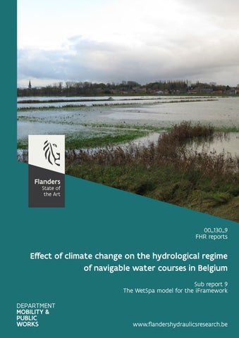
Cover figure © The Government of Flanders, Department of Mobility and Public Works, Flanders Hydraulics Research Legal notice Flanders Hydraulics Research is of the opinion that the information and positions in this report are substantiated by the available data and knowledge at the time of writing. The positions taken in this report are those of Flanders Hydraulics Research and do not reflect necessarily the opinion of the Government of Flanders or any of its institutions. Flanders Hydraulics Research nor any person or company acting on behalf of Flanders Hydraulics Research is responsible for any loss or damage arising from the use of the information in this report. Copyright and citation © The Government of Flanders, Department of Mobility and Public Works, Flanders Hydraulics Research 2021 D/2021/3241/024 This publication should be cited as follows: Salvadore, E.; Nossent, J.; Pereira, F.; Mostaert, F. (2021). Effect of climate change on the hydrological regime of navigable water courses in Belgium: Sub report 9 – The WetSpa model for the iFramework. Version 1.0. FHR Reports, 00_130_9. Flanders Hydraulics Research: Antwerp Reproduction of and reference to this publication is authorised provided the source is acknowledged correctly. Document identification Customer: Keywords (3-5): Knowledge domains: Text (p.): Confidential: Author(s):

Flanders Hydraulics rzesearch Ref.: WL2021R00_130_9 climate change; hydrological impact analysis; distributed & lumped models; Belgium; model uncertainty Watermanagement > hydrology > numerical modelling 17 ‫ ܈‬No

Appendices (p.): ‫ ܈‬Available online

Salvadore, E.

Control Name Reviser(s):

Project leader:

Nossent, J.; Pereira, F.

Pereira, F.

Signature Getekend door:Jiri Nossent (Signature) Getekend op:2022-03-22 09:46:19 +01:0 Reden:Ik keur dit document goed

Getekend door:Fernando Pereira (Signat Getekend op:2022-03-22 08:49:20 +01:0 Reden:Ik keur dit document goed

Getekend door:Fernando Pereira (Signat Getekend op:2022-03-22 08:50:04 +01:0 Reden:Ik keur dit document goed

Approval Mostaert, F. Head of Division:

F-WL-PP-16.03.01-02 Valid as from 6/11/2021

For the Head of Division, absent Patrik Peeters, Engineer, in charge with leading the Division Flanders Hydraulics Research

Digitaal ondertekend Patrik Peeters Patrik Peeters door (Signature) (Signature) Datum: 2021.09.08 08:17:18 +02'00'

Effect of climate change on the hydrological regime of navigable water courses in Belgium - Sub report 9 – The WetSpa model for the iFramework

Abstract The assessment of climate change impact on the hydrological system is becoming more and more a key issue for establishing best management practices for the limited water resources. Climate change impact analysis requires state of the art hydrological models to perform simulations of different climate scenarios. The study of these scenarios is however not sufficient to compensate for the high uncertainty of future forecasting. With the purpose of including model structure uncertainty, the iFramework was developed (Pannemans et al., 2014). This Python-based framework is a powerful platform for managing and creating flexible hydrological models. Within the iFramework, three well known lumped hydrological models can be used: NAM, PDM and VHM. The available tools have however a lumped model structure which can be a limiting factor for complex hydrological applications. To overcome this limitation, we extended the library of hydrological tools by including the spatially-distributed model WetSpa in the iFramework toolbox. This report describes the development of a iFramework-compatible WetSpa model, and its implementation and testing by means of theoretical and real case study. The WetSpa model (Water and energy transfer between Soil plant and atmosphere) is a well established GIS-based, spatially-distributed rainfall-runoff model for hydrological simulations at the catchment scale. Recently a process-based Python version of the model has been developed (Salvadore, E. et al., 2012, 2014), this new version is based on a different Python framework (Schmitz, et al. 2013a, 2013b) but facilitates the integration with the iFramework. To perform the integration, we carried out an in-depth comparison of the two framework paradigms to identify the appropriate strategy to bridge the gaps between the two frameworks. Afterwards, we developed new Python codes for the WetSpa model in the iFramework and we modified some parts of the iFramework to allow the integration of the WetSpa model in the toolbox. In this phase, we decided to develop two versions of the WetSpa model: a spatially-distributed and a lumped version. Distributed and lumped WetSpa models share the same Python codes, the main difference is the flow routing approach. Finally, these two versions were verified by means of a theoretical and a real case study. We compared the results generated by the two model versions with the original WetSpa-Python model. In both validation tests, the spatially-distributed model produced nearly identical results to the original model, with only negligible rounding errors. In the lumped model, all the inputs and parameters were averaged over the all catchment. The validation of the lumped model is less straightforward as model parameters partially lose their physical meaning and cannot be directly compared with the distributed ones. However, by modifying a number of parameters we were able to achieve a good match between the lumped model and the original spatially-distributed model, which ensure the correct implementation of the model code. Further tests on the lumped model are however required for a better understanding of the behavior of the model parameters.

Final version

WL2021R00_130_9

III

F-WL-PP-16.03.01-02 Valid as from 6/11/2021

Effect of climate change on the hydrological regime of navigable water courses in Belgium Sub report 9 – The WetSpa model for the iFramework

Contents Abstract ............................................................................................................................................................ III Contents ............................................................................................................................................................ V List of tables...................................................................................................................................................... VI List of figures ................................................................................................................................................... VII 1

Introduction and Report Structure ............................................................................................................ 1

The WetSpa model .................................................................................................................................... 2

2.1

The original WetSpa model ............................................................................................................... 2

2.2

The WetSpa-Python model................................................................................................................ 3

The WetSpa model for the iFramework .................................................................................................... 4 3.1

The iFramework and the WetSpa framework ................................................................................... 4

3.2

Technical Implementation ................................................................................................................. 6

3.3

Model Validation: application to case studies .................................................................................. 8

3.3.1

Fully distributed model.............................................................................................................. 9

3.3.2

Lumped model ......................................................................................................................... 11

Conclusions and Recommendations ............................................................................................................... 16 References ....................................................................................................................................................... 17 Appendix A: Step-by-Step User Manual .......................................................................................................... A1 Appendix B: iFramework modifications .......................................................................................................... A9

Final version

WL2021R00_130_9

Effect of climate change on the hydrological regime of navigable water courses in Belgium Sub report 9 – The WetSpa model for the iFramework

List of tables Table 1 – Comparison between the iFramework and available models, and the WetSpa-Python model and its framework. ........................................................................................................................................................ 4 Table 2 – Comparison between the WetSpa-Python component names and the WetSpa components in the iFramework........................................................................................................................................................ 6 Table 3 – Maximum absolute error in the water balance [m] between the developed spatially-distributed WetSpa model for the iFramework and the original WetSpa-Python model code. ....................................... 11 Table 4 – Default soil type classification of the WetSpa model ...................................................................... A2 Table 5 – Default land use classification of the WetSpa model ...................................................................... A3 Table 6 – Default parameters characterizing soil textural classes in the WetSpa model ............................... A3 Table 7 – Default parameters characterizing land use classes of the WetSpa model .................................... A4 Table 9 – WetSpa state variables .................................................................................................................... A7

WL2021R00_130_9

Final version

Effect of climate change on the hydrological regime of navigable water courses in Belgium Sub report 9 – The WetSpa model for the iFramework

List of figures Figure 1 – At every time step, the WetSpa model performs a water balance at cell level, the main considered processes are here illustrated. .......................................................................................................................... 2 Figure 2 - The structure of the WetSpa-Python model is process-based, the model components interact with each other at run time and variable exchanges are managed at a higher level by the Python modelling framework. Grey boxes represent the main WetSpa-Python components and arrows represent the main links within components. ........................................................................................................................................... 3 Figure 3 – The WetSpa-Python model generates (a) spatially-distributed response functions of instantaneous precipitation or (b) the total catchment response function ............................................................................. 7 Figure 4 – Theoretical case study: spatial inputs............................................................................................... 8 Figure 5 – Theoretical case study: average precipitation time series ............................................................... 8 Figure 6– Kleine Nete case study: spatial inputs and average precipitation time series .................................. 9 Figure 7 – The developed code for the spatially-distributed WetSpa model and the original WetSpa-Python code produce identical results for the theoretical case study. Results refer to the catchment outlet. ......... 10 Figure 8 – The developed code for the spatially-distributed WetSpa model and the original WetSpa-Python code produce identical results for the Kleine Nete catchment. Results refer to the catchment outlet......... 10 Figure 9 – The lumped WetSpa model seems to correctly predict the evolution of soil moisture content and the general trends of other water balance components before saturation. During saturation infiltration is overestimated by 1 [mm] due to and overestimation of percolation (groundwater recharge). .................... 12 Figure 10 – The results of the lumped WetSpa model for surface runoff, infiltration and percolation, matches very well the predictions of the distributed WetSpa model when a constant map of hydraulic conductivity is used in the latter. The soil moisture content is however affected by this parameter modification. ............. 12 Figure 11 – The results of the lumped WetSpa model perfectly matches the predictions of the distributed WetSpa model when constant parameter maps are used in the latter. ......................................................... 13 Figure 12 – The routing components of the lumped model produce similar results to the spatially-distributed model, the only exception is the groundwater discharge. .............................................................................. 14 Figure 13 – The lumped WetSpa model seems to correctly predict the evolution of soil moisture content and the general trends of other water balance components before saturation. During saturation surface runoff is significantly underestimated due to and overestimation of depression storage. .......................................... 15 Figure 14 – The routing components of the lumped model produce generally good results compared to the spatially-distributed model, particularly for interflow and the total flow. However overland flow is significantly underestimated due to the incorrect calculation of the surface runoff component as well as the groundwater discharge. .................................................................................................................................. 15 Figure 15 – iFramework folders structure ....................................................................................................... A2

Final version

WL2021R00_130_9

VII

Effect of climate change on the hydrological regime of navigable water courses in Belgium Sub report 9 – The WetSpa model for the iFramework

1 Introduction and Report Structure The iFramework is a powerful platform for managing and creating flexible hydrological models (Pannemans et al., 2014). Within the iFramework, three well known lumped hydrological models can be used: NAM, PDM and VHM. This approach allows the study of climate change with an ensemble of model structures, in view of uncertainty reduction. However, all the available tools have a lumped model structure and this can be a limitation for complex applications. To overcome this limitation, we included the spatially-distributed model WetSpa in the iFramework toolbox. The main objective of this project is the development of a WetSpa model version which is compatible with the requirements of the iFramework and to test this implementation by means of a theoretical and a real case study. This report is divided into three chapters and two appendices. Chapter 1 introduces the original spatially-distributed hydrological model WetSpa and its Python version. Chapter 2 deals with the implementation of the WetSpa model in the iFramework: Section 2.1 compares the iFramework with the Python framework used by the WetSpa model and identifies the necessary modifications to achieve the objective; Section 2.2 gives details of the technical implementation; Section 3.3 presents the results of the model validation. Chapter 3 summarizes the conclusion of this project and provides the ‘lessons learned’. Appendix A is the step-by-step user guide for running the WetSpa-Python for the iFramework. Appendix B reports all the modifications we made to the iFramework in order to include the WetSpa model in the list of available tools.

Final version

WL2021R00_130_9

Effect of climate change on the hydrological regime of navigable water courses in Belgium Sub report 9 – The WetSpa model for the iFramework

2 The WetSpa model This chapter introduces the main characteristics and modeling concepts of the WetSpa model. Section 1.1 gives a short introduction of the original WetSpa model and section 1.2 describes the new Python version of the WetSpa model.

2.1 The original WetSpa model The WetSpa model is a GIS-based, spatially-distributed rainfall-runoff model for hydrological simulations at the catchment scale. WetSpa stands for “Water and energy transfer between Soil, plant and atmosphere”. The model has a relatively long history dating back to 1996 (Wang et al. 1996) and it has been used and modified ever since for a wide range of applications (Liu et al., 2006; Chormanski et al., 2008; Berezowski et al., 2012; Verbeiren et al., 2013; Tavakoli et al., 2013). Moreover, the WetSpa model code was recently tested in the Distributed Model Intercomparison Project (Safari et al., 2012). The model calculates the water balance at the raster cell level and simulates several physical processes with a cascade approach (Figure 1). Liu and De Smedt (2005) describe the main physically-based equations solved by the model, of which hereafter only a short summary is given. Surface runoff is produced using a modified runoff coefficient method. Based on the geomorphological characteristic of each raster cell, the runoff is then routed as overland and channel flow with the linear diffusive wave approximation and the geomorphological instantaneous unit hydrograph concept (G-IUH). Based on Darcy’s law and the kinematic approximation, the model calculates interflow as a function of the effective hydraulic conductivity and the hydraulic gradient, while groundwater flow is estimated with the linear reservoir method on small sub-catchment scale as a function of groundwater storage and a recession coefficient. Time step resolution of inputs and outputs ranges from one hour to days, months and years.

Rainfall Evapotranspiration

Interception

River Flow

Net Rainfall Depression Unsaturated soil

Runoff

Infiltration Interflow Deep percolation

Saturated soil

Groundwater flow and discharge

Figure 1 – At every time step, the WetSpa model performs a water balance at cell level, the main considered processes are here illustrated.

The WetSpa model is composed of three components: two pre-processing components and the main simulation code. The two pre-processing components are: (a) the GIS-based parameter maps estimator and (b) the G-IUH routine. The inputs of the model are: (a) precipitation, potential evapotranspiration and

WL2021R00_130_9

Final version

Effect of climate change on the hydrological regime of navigable water courses in Belgium Sub report 9 – The WetSpa model for the iFramework

temperature time series, which are distributed over the catchment with the Thiessen polygons method; and (b) spatially distributed parameters, which are derived on basis of three maps: topography, soil texture and land use. Typical outputs are: flow hydrographs at catchment and sub-catchment outlets, and maps of major water fluxes for each time step. Calibration can be manually or automatically performed by modifying the 11 global calibration parameters. Automatic calibration is performed with the model independent Parameter ESTimator (PEST) software (Liu et al. 2005). Recently, Shafii and de Smedt (2009) also tested multi-objective calibration with a genetic algorithm.

2.2 The WetSpa-Python model The WetSpa-Python model (Salvadore, E. et al., 2012, Salvadore, E. et al., 2015) is essentially a reimplementation of the original WetSpa model according to the Python modelling framework standards developed by Schmitz, et al. (2013a, 2013b). However, both the model structure and the programming language are sensibly different from the original model, while the main semi-physical equations are preserved. The new model structure is modular and process-based. Every hydrological process is coded in a separate module and modules exchange data during running time through the Python modelling framework prototype (Figure 2). The framework allows model components to run with independent time steps. In other words, hydrological processes in the WetSpa-Python model can be simulated at different time resolution according to data availability and physical scale of the hydrological process. Moreover, the simulation time step is no longer limited to 1 hour. Spatial resolution is purely a function of the input data: the finer the data the more detailed the model. The two pre-process components of the original WetSpa model are integrated in the new system as static components of the framework and they run automatically at the start of the simulation. Calibration parameters Spatially-distributed data & Parameters

Rain

IUH

PET

Atmosphere

Interception Surface

Flow Routing (Surface & Interflow)

Surface Runoff & Infiltration

Depression Losses

Interflow

Soil Evaporation

Groundwater Routing Total Discharge

Groundwater Recharge

Soil Moisture Content

Catchment Water Balance

GIS pre-process

Time series

Unsaturated zone Saturated zone

Outputs Modelling framework

Figure 2 - The structure of the WetSpa-Python model is process-based, the model components interact with each other at run time and variable exchanges are managed at a higher level by the Python modelling framework. Grey boxes represent the main WetSpa-Python components and arrows represent the main links within components.

Final version

WL2021R00_130_9

Effect of climate change on the hydrological regime of navigable water courses in Belgium Sub report 9 – The WetSpa model for the iFramework

3 The WetSpa model for the iFramework This chapter deals with the main objective of this project: the implementation of the spatially-distributed hydrological model WetSpa in the iFramework. We refer the reader to (Pannemans et al., 2014) for a detailed description of the iFramework, which is out of the scope of the present report. Section 2.1 compares the iFramework concept with the Python framework used by the WetSpa model, and identifies the necessary modifications. Section 2.2 gives a technical description of the implementation of the WetSpa model in the iFramework and finally Section 2.3 provides a series of example applications.

3.1 The iFramework and the WetSpa framework The iFramework and the WetSpa framework sensibly differ (Table 1). Therefore both the WetSpa-Python and the iFramework codes required adaptations to achieve the objective. The main needed adaptations relate to: - computer language versions  we decided to use the most recent Python and PCRaster versions (the ones used by the iFramework); - variable names  when possible, we modified the variable names to be as consistent as possible with the standards of the iFramework (e.g. surface runoff “qs” in WetSpa-Python becomes “OF” in the WetSpa model for the iFramework); - variable types  calculations are performed using PCRaster maps wherever possible, as it is done by the other models in the iFramework. For complex WetSpa model calculations (i.e. surface flow routing) NumPy arrays are used. - static components of the WetSpa-Python model cannot be implemented in a straightforward way in the iFramework  we coded the static components as stand-alone Python files (not according to the iFramework standards); - lumped and distributed models share the same code in the iFramework, while only a distributed version of the WetSpa model exists  we developed two versions of the WetSpa model (a) fully-distributed, and (b) lumped. These two versions share the same code for the six process-based components, however we developed new codes for the routing of overland flow and groundwater; - iFramework code requires modifications to accommodate the WetSpa model  we kept these modifications to the minimum, a full list is provided in Appendix B.

Table 1 – Comparison between the iFramework and available models, and the WetSpa-Python model and its framework.

iFramework & models

WetSpa-Python and its framework

Global variables are stored in DM (Dynamic Local variables are used in every model Model object). component. → Variables have the same name in every → Different names can be used in different component. components.

WL2021R00_130_9

Final version

Effect of climate change on the hydrological regime of navigable water courses in Belgium Sub report 9 – The WetSpa model for the iFramework

→ The iFramework does not exchange variables → The framework exchanges variables between between components. components at run time DM

Submodel 1

A  A1

A1 = f(A)

A Submodel 1

A1 A1

Submodel 2

B1 = f(A1,B)

Submodel 2

B  B1

B1 = f(A1,B)

→ Components are not fully independent and → Components are fully independent and links between components are explicit. there are no explicit links between them. All sub-modules must have the same temporal Model components can have different spatial and and spatial discretization temporal discretization Language and GIS software: Python 2.7 and Language and GIS software: Python 2.5.4 and PCRaster 4.0 PCRaster 3.0 Sub-modules can be add at run time

Model components cannot be added at run time

Manual parameter-maps preprocess

Automated parameter-maps preprocess

Models in the framework can be run in lumped or Only a distributed code exists for the WetSpadistributed mode without code modification Python model. The user needs to modify the iFramework in The user does not need to modify the framework to add a new model component. order to add a new sub-module Many functions are available for evaluation and automatic calibration

model No code is available for model evaluation and automatic calibration

Parameters (and variables) are global and they Parameters are local and they are declared within are stored in the object pBox the particular model component Variables are overwritten at every time step

Variables can be overwritten or can be stored over time

State variables are “single value” (lumped State variables are of the type NumPy masked models) or arrays (distributed models) array. Sub-modules are Python classes included in the Model components are Python classes and are main model script. stored in separate scripts and folders. The order of calculation of the different sub- The order of calculation of the model modules is selected by the user. components is selected by the framework according to the dependences between components.

Final version

WL2021R00_130_9

Effect of climate change on the hydrological regime of navigable water courses in Belgium Sub report 9 – The WetSpa model for the iFramework

3.2 Technical Implementation The WetSpa model for the iFramework consists of three Python files: WetSpaGIS.py, WetSpaIUH.py, and myWetSpaModel.py. The first two files are independent from the iFramework and can be considered as model pre-processing, while the third represents the real model and all the process-based components are coded in this file as Python classes. For those familiar with the WetSpa-Python model structure, Table 2 provides a comparison of file names. Table 2 – Comparison between the WetSpa-Python component names and the WetSpa components in the iFramework.

WetSpa-Python model components (Python files) static_preproc.py dynamic_preproc.py

WetSpa for the iFramework: independent codes, Python classes in myWetSpamModel.py, or modification of other Python files WetSpaGIS.py (independent from the iFramework)

iuh_standard.py

WetSpaIUH.py (independent from the iFramework)

Rain.py PET.py

Modification of iFramework.py and configuration.txt

Interception.py

WetSpaInterception (Python class)

RainExcess_Infiltration.py

WetSpaRainExc_Infil (Python class)

Depression_Overlandflow.py

WetSpaDepression (Python class)

Interflow.py

WetSpaInterflow (Python class)

Evapotranspiration_soil.py

WetSpaSoilEvaporation (Python class)

Groundwater_recharge.py

WetSpaPercolation (Python class)

Balance.py

WetSpaBalance (Python class)

output.py

WetSpaBalanceOutput (Python class)

Flow_routing.py

WetSpaUZRouting (Python class) WetSpaUZRoutingL (Python class) lumped

Linear_reservoirs.py

WetSpaBZRouting (Python class) WetSpaBZRoutingL (Python class) lumped

Two types of WetSpa-Python components could not be converted into iFramework sub-modules: (1) static components, and (2) components dealing with meteorological inputs. (1) Static components are not supported by the iFramework as all the sub-modules of a dynamic model must share the same temporal

WL2021R00_130_9

Final version

Effect of climate change on the hydrological regime of navigable water courses in Belgium Sub report 9 – The WetSpa model for the iFramework

resolution. We therefore created two stand-alone pre-processing files: WetSpaGIS.py and WetSpaIUH.py. The first file generates all the necessary parameter maps (or a single value in the lumped mode) for the WetSpa model. The second file generates a stack of maps (or a time series in the lumped mode) of instantaneous response functions (Figure 3) which are used in the routing process. (2) Components dealing with meteorological inputs do not exist in the iFramework as the iFramework internally manipulates these inputs. We therefore used the existing iFramework functionalities for input manipulation. There are three possible ways for loading meteorological data (method loadMeteoData_initial() in iFramework.py), none of these approaches however allows the distribution of precipitation (and/or potential evapotranspiration) time series according to a Thiessen polygon map (default approach in the WetSpa model). We therefore modified the loadMeteoData_initial() method of the iFramework, by adding this option. Consequently a new directive was added to the configuration.txt with the name METEODATA_THIESSEN.

(a) Spatially-distributed model

(b) Lumped model Combined catchment response Q

time

y x

Figure 3 – The WetSpa-Python model generates (a) spatially-distributed response functions of instantaneous precipitation or (b) the total catchment response function

The file myWetSpaModel.py contains the WetSpa model code. Following the examples of the NAM, PDM and VHM models we divided the WetSpa model code into 14 classes. Two classes represent the distributed and the lumped models, respectively WetSpaModel and WetSpaModelLumped. In these two model classes 10 sub-modules, the model constants and parameters, and the model variables are listed. The two classes are composed of two methods: intial and dynamic. In the intial method, variables and parameters are initialized. In the dynamic method, the dynamic methods of all the sub-modules are called and the total flow is calculated as the sum of surface flow, interflow and groundwater flow. Distributed and lumped WetSpa models share 6 sub-modules, the two routing models are different for the two model versions and catchment averages are not calculated in the lumped model.

Final version

WL2021R00_130_9

Effect of climate change on the hydrological regime of navigable water courses in Belgium Sub report 9 – The WetSpa model for the iFramework

3.3 Model Validation: application to case studies We validated the spatially-distributed and the lumped WetSpa models by means of two case studies: a theoretical case and a real case. The theoretical catchment has a square shape and covers an area of 625 km2, input data has a spatial resolution of 5X5 km. The catchment has a very simple topography (Figure 4 (a)) ranging from 0 to 3 m and a very diverse land cover and soil texture (Figure 4 (b), (c)).

Figure 4 – Theoretical case study: spatial inputs

The simulation time step is 1 [h] and the total length of the simulation is 150 [h]. Precipitation has either gradual (1 [mm/h]) or sharp (10 [mm/h]) increases/decreases as shown in Figure 5. Precipitation [mm] 12 10 8 6 4 2 0

120

150 Time [h]

Figure 5 – Theoretical case study: average precipitation time series

The real case is the 581 km2 Kleine Nete catchment, Belgium. The basin is relatively flat, with topography ranging from 3 to 48 [m] and an average slope of 0.36% (Figure 6 (a)). The land use is dominated by grassland and agriculture (total of 49%), while 23% of the catchment is urbanized and the remaining area is covered by forests (Figure 6(b)). The most diffuse soil types are sand, loamy-sand and sandy-loam, followed by sandyclay loam and silt and clay (Figure 6 (c)). The spatial resolution of the input maps is 50 [m]. The simulated period is nearly 1 month with a daily time step (Figure 6 (d)).

WL2021R00_130_9

Final version

Effect of climate change on the hydrological regime of navigable water courses in Belgium Sub report 9 – The WetSpa model for the iFramework

(a) Topography [m]

(b) Land use

(d) Precipitation [mm]

48.5

5.5

50 Time [d]

Figure 6– Kleine Nete case study: spatial inputs and average precipitation time series

3.3.1

Fully distributed model

Model results of the spatially-distributed WetSpa model for the iFramework are compared with results generated by the original WetSpa-Python model. For both models, no calibration has been performed. At this stage, we intend to prove the correctness of the developed code for the iFramework and not its predictive performances. The developed code and the original WetSpa-Python code produce identical results for both the theoretical and the real case study. In Figure 7 (theoretical case) and Figure 8 (real case) in fact, the curves representing overland flow, interflow, groundwater discharge and total flow at the catchment outlet perfectly overlay. Rounding effects produce only negligible errors in the catchment average water balance (Table 3).

Final version

WL2021R00_130_9

Effect of climate change on the hydrological regime of navigable water courses in Belgium Sub report 9 – The WetSpa model for the iFramework

Overland flow [m3/s]

Interflow [m3/s]

0.03

0.02

20 0.01

10 0

120

0 0

150 Time [h]

1.2

0.8

0.4

10 30

120

150

Total discharge [m3/s]

1.6

Time [h]

Groundwater discharge [m3/s]

150 Time [h]

120

150 Time [h]

Figure 7 – The developed code for the spatially-distributed WetSpa model and the original WetSpa-Python code produce identical results for the theoretical case study. Results refer to the catchment outlet.

Overland Flow [m3/s]

Interflow [m3/s] 30

50 Time [d]

0 10

50 Time [d]

Total discharge [m3/s]

Groundwater Discharge [m3/s] 50

30 10 20 5 0

10 0

50 Time [d]

Figure 8 – The developed code for the spatially-distributed WetSpa model and the original WetSpa-Python code produce identical results for the Kleine Nete catchment. Results refer to the catchment outlet.

WL2021R00_130_9

Final version

Effect of climate change on the hydrological regime of navigable water courses in Belgium Sub report 9 – The WetSpa model for the iFramework Table 3 – Maximum absolute error in the water balance [m] between the developed spatially-distributed WetSpa model for the iFramework and the original WetSpa-Python model code.

Catchment averages

3.3.2

Theoretical case

Kleine Nete case

Precipitation

0.000

PET

0.000

Depression

0.0001

1E-06

Interception

0.00029

0.000

Soil Moisture

0.05

0.005

Infiltration

0.0002

0.000

Evaporation from Interception Storage

0.0003

0.000

Evaporation from Unsaturated Soil

0.001

0.0001

Evaporation from Depression Storage

0.0003

1E-06

Evaporation from Saturated Soil

0.000

0.0001

Percolation

0.000

0.001

Surface Runoff

0.001

0.000

Interflow

1E-06

0.001

Groundwater Flow

1E-05

0.001

Lumped model

The lumped version of the WetSpa model solves the same semi-physical equations for calculating the water balance. It however calculates this balance at the catchment level and not for every grid cell. Distributed inputs and parameters are therefore averaged in the preprocessing phase. To evaluate the developed lumped WetSpa model, we first compare the calculated components of the water balance with the ones produced by the distributed model (Figure 9). Even if the lumped model considers the catchment as one grid cell of 25X25 km, it seems to correctly predict the soil moisture content and the general trends of other water balance components before saturation occurs (first 40 minutes of the simulation). However during saturation, surface runoff is underestimated and infiltration is overestimated by about 1 mm. At saturation the system is in quasi steady state condition and the error is due to an incorrect estimation of percolation (groundwater recharge), which allows a higher infiltration. In the WetSpa model, percolation is mainly governed by the vertical hydraulic conductivity, which in turn is dependent on soil characteristics. In this particular theoretical case, soil texture significantly varies, i.e. clay and sandy soils. The hydraulic conductivity of these two soil classes differs a factor 103 (Table 6 in Appendix A). To verify the hypothesis that the spatial distribution of the hydraulic conductivity is responsible for the differences in the water balance results, we compared the lumped results with a distributed WetSpa model that uses an average constant map of hydraulic conductivity (Figure 10). The results of the lumped WetSpa model for surface runoff, infiltration and percolation, matches very well the predictions of the distributed WetSpa model when a constant map of hydraulic conductivity is used in the latter. The soil moisture content is however affected by this parameter modification. The spatial distribution of parameter values has a great influence on model results. This conclusion is justifiable as parameters in the lumped model partially lose their physical meaning. To the best knowledge of the authors, there is no simple and generally accepted relation to convert distributed parameters into lumped parameters. Therefore, the simple choice of using parameter averages

Final version

WL2021R00_130_9

Effect of climate change on the hydrological regime of navigable water courses in Belgium Sub report 9 – The WetSpa model for the iFramework

might generate significant errors in the model predictions. Parameters in the lumped models need recalibration to correctly estimate the water balance. Very likely, standard calibration techniques, used for the spatially-distributed model, cannot be directly applied to the lumped model, more tests are therefore required to establish a proper technique for model calibration. Soil Moisture [mm]

Surface Runoff [mm]

230 6 200

170

140

120

150 Time [h]

Infiltration [mm]

120

150 Time [h]

120

150 Time [h]

Percolation [mm] Lumped

Distributed 4

120

150 Time [h]

Figure 9 – The lumped WetSpa model seems to correctly predict the evolution of soil moisture content and the general trends of other water balance components before saturation. During saturation infiltration is overestimated by 1 [mm] due to and overestimation of percolation (groundwater recharge).

Soil Moisture [mm]

Surface Runoff [mm]

230 6 200

170

140 0

120

150 Time [h]

Infiltration [mm]

120

150 Time [h]

120

150 Time [h]

Percolation [mm] Lumped

Distributed 4

120

150 Time [h]

Figure 10 – The results of the lumped WetSpa model for surface runoff, infiltration and percolation, matches very well the predictions of the distributed WetSpa model when a constant map of hydraulic conductivity is used in the latter. The soil moisture content is however affected by this parameter modification.

WL2021R00_130_9

Final version

Effect of climate change on the hydrological regime of navigable water courses in Belgium Sub report 9 – The WetSpa model for the iFramework

As a final verification of the water balance calculation, we compared the results of the lumped model with the ones produced by the distributed model using constant maps for all the parameters (Figure 11). A perfect match is achieved for every component of the water balance. Since the instantaneous values of the water balance components are identical for the distributed and the lumped models, we can independently test the implementation of the flow routing component (Figure 12). Surprisingly, also in this case the lumped model is able to reproduce accurately the results of the distributed model for the overland flow and the interflow components. The modified G-IUH calculation for the lumped model is therefore able to accurately mimic the distributed routing for this simple theoretical case. The groundwater discharge is the routing component that is mostly affected by the simplified lumped approach. Groundwater discharge is calculated at the subcatchment level with the linear reservoirs method as a function of groundwater storage and a recession coefficient. In the lumped approach no sub-catchment can be identified, therefore the catchment responds as one large reservoir. The recession coefficient therefore needs recalibration.

Soil Moisture [mm]

Surface Runoff [mm]

230 6 200

170

140

120

150 Time [h]

Infiltration [mm]

120

150 Time [h]

120

150 Time [h]

Percolation [mm] Lumped

Distributed 4

120

150 Time [h]

Figure 11 – The results of the lumped WetSpa model perfectly matches the predictions of the distributed WetSpa model when constant parameter maps are used in the latter.

Final version

WL2021R00_130_9

Effect of climate change on the hydrological regime of navigable water courses in Belgium Sub report 9 – The WetSpa model for the iFramework

Overland flow [m3/s]

Interflow [m3/s]

0.04 0.03

0.02 10 0

0.01 0

120

150 Time [h]

120

150 Time [h]

Total discharge [m3/s]

Groundwater discharge [m3/s] 30

Lumped

Distributed

120

150 Time [h]

20 10 0

120

150 Time [h]

Figure 12 – The routing components of the lumped model produce similar results to the spatially-distributed model, the only exception is the groundwater discharge.

The lumped model applied to the Kleine Nete case generates similar results (Figure13). As in the theoretical case, the soil moisture seems very well estimated, infiltration is also correctly predicted. Surface runoff is significantly underestimated due to the effect of spatial distributed parameters regulating the calculation of depression storage. The underestimation of surface runoff produces an underestimation of overland flow, while the correct estimation of the soil moisture content produces very good results for the interflow calculation. The general trend of groundwater discharge is also well captured although the absolute values differ 1 to 3 m3/s (Figure 14).

WL2021R00_130_9

Final version

Effect of climate change on the hydrological regime of navigable water courses in Belgium Sub report 9 – The WetSpa model for the iFramework

Soil Moisture [mm]

Surface Runoff [mm]

1.6 1.2

0.8 55

0.4 0

40 50 Time [d]

Infiltration [mm]

Lumped

Distributed

40 50 Time [d]

Depression [mm]

0.8 0.6

0.4 0.2

40 50 Time [d]

Figure 13 – The lumped WetSpa model seems to correctly predict the evolution of soil moisture content and the general trends of other water balance components before saturation. During saturation surface runoff is significantly underestimated due to and overestimation of depression storage.

Overland flow [m3/s]

Interflow [m3/s] 30

6 20

2 0 0

0 0

Time [d]

Lumped

Groundwater discharge [m3/s]

Distributed 60

Total discharge [m3/s]

10 0

5 0 0 0

0 0

50 Time [d]

Figure 14 – The routing components of the lumped model produce generally good results compared to the spatially-distributed model, particularly for interflow and the total flow. However overland flow is significantly underestimated due to the incorrect calculation of the surface runoff component as well as the groundwater discharge.

Final version

WL2021R00_130_9

Effect of climate change on the hydrological regime of navigable water courses in Belgium Sub report 9 – The WetSpa model for the iFramework

Conclusions and Recommendations Climate change impact analysis is greatly affected by uncertainty. Future predictions of climate variables are generally produced as an ensemble of possible scenarios to reduce the uncertainty generated by the model inputs. A similar approach should be considered to deal with model structure uncertainty. The iFramework is a PCRaster-Python toolbox that allows multi-model simulations. The hydrological models available in the iFramework toolbox have however a lumped model structure. The main objective of the project was to extend the library of hydrological tools of the iFramework, by including the spatially-distributed model WetSpa. Starting from the Python version of the WetSpa model, (1) we compared the iFramework concepts with the Python framework used by WetSpa-Python model in detail; (2) we selected appropriate strategies to bridge the gaps between the two frameworks; (3) we developped new codes for the WetSpa model in the iFramework and we modified some parts of the iFramework to allow the integration of the WetSpa model in the toolbox; and finally (4) we tested the correctness of the developed codes by mean of theoretical and real case studies. (1) The iFramework and the Python framework used by the WetSpa model are different but comparable with respect to the general concepts of modularity and flexibility. Model components of the WetSpa-Python model are fully independent and can be easily replaced with newly developed model components or with existing models without modification of the framework code. Furthermore, model components can have different spatial and temporal resolution and the framework takes care of the correct order of calculation. These characteristics are only partially included in the iFramework options. However, the iFramework has other important options such as an extended library of automated calibration algorithms, three lumped models are included in the toolbox and scripts for input and output manipulation are available. (2) We adapted as much as possible the WetSpa-Python code to fulfill the requirements of the iFramework, limiting to a minimum the modification of the iFramework itself. Computer language, variable names, variable types were changed to the iFramework standards. Static WetSpa components were re-coded as stand-alone Python files. We moreover decided to develop two version of the WetSpa model: a spatiallydistributed and a lumped version to take full advantage of the iFramework concept. (3) Starting from the WetSpa-Python code we developed three new Python scripts: two for pre-processing and the myWetSpaModel.py. Pre-processing scripts create parameter maps (or single values in the lumped mode) and calculate the G-IUH (geomorphologic instantaneous unit hydrograph). The model code of WetSpa follows the example of the existing NAM, PDM and VHM model for the iFramework. The myWetSpaModel.py file contains 14 classes: two model classes, 10 process-based components and two classes dealing with the water balance. Distributed and lumped WetSpa models share 6 sub-modules, while they differ for the routing approach and the lumped model does not need to calculate catchment averages. (4) We tested the lumped and the spatially-distributed models by means of two examples: a theoretical case and a real case. We compared the results generated by the two model versions with the original WetSpaPython model. In both validation tests, the spatially-distributed model produced nearly identical results to the original model, with only negligible rounding errors. In the lumped model, all the inputs and parameters were averaged over the all catchment. The validation of the lumped model is less straightforward as model parameters partially lose their physical meaning and cannot be directly compared with the distributed ones. However, by modifying a number of parameters we were able to achieve a good match between the lumped model and the original spatially-distributed model. Further tests on the lumped model are however required for a better understanding of the behavior of the model parameters.

WL2021R00_130_9

Final version

Effect of climate change on the hydrological regime of navigable water courses in Belgium Sub report 9 – The WetSpa model for the iFramework

References Berezowski, T., Chormanski, J., Batelaan, O., Canters, F., Van de Voorde, T., 2012. Impact of remotely sensed land-cover proportions on urban runoff prediction. International Journal of Applied Earth Observation and Geoinformation, 16, pp. 54-65. Chormanski, J., Van de Voorde, T., De Roeck, T., Batelaan, O., Canters, F., 2008. Improving distributed runoff prediction in urbanized catchments with remote sensing based estimates of impervious surface cover. Sensors, 8(2), pp. 910-932. Liu, Y. B., De Smedt, F., 2005. Flood Modeling for Complex Terrain Using GIS and Remote Sensed Information. Water Resource Management, 19, pp. 605-624. Liu, Y. B., Gebremeskel, S., De Smedt, F., Hoffman, L., Pfister, L., 2006. Predicting storm runoff from different land-use classes using a geographical information system-based distributed model. Hydrological Processes, 20(3), pp. 533-548. Pannemans, B., 2014. Deelopdracht 1: hydrologische neerslagfvoermodellen. Next-generation tools m.b.t. hydrometrie, hydrologie en hydraulic in het operationele waterbeheer – fase 1: analyse. Vlaamse Milieumaatschappij – Afdeling Operationeel Waterbeheer, International Marine & Dredging Consultants, Antwerp, Belgium. Document: K:\PROJECTS\11\11432 – Next-generation tools\10Rap\RA14097_NextGen_DO1_hydrologisch_model_v0.6.docx. Salvadore, E., Bronders, J., Batelaan, O., 2012. Enhanced model flexibility and coupling opportunities: the WetSpa model case. iEMSs 2012, Leipzig, Germany, 01-05/07/2012. Salvadore, E., Bronders, J., Schmitz, O., van der Kwast, J., Batelaan, O, 2015. Process-based hydrological modeling: the WetSpa-Python model, to be submitted in environmental Modeling and Software. Safari, A., De Smedt, F. & Moreda, F., 2012. WetSpa model application in the Distributed Model Intercomparison Project (DMIP2). Journal of Hydrology, 418, pp. 78-89. Schmitz, O., Karssenberg, D., de Joong, K., de Kok, J. L., de Jong, S. M., 2013a. Map algebra and model algebra for integrated model building. Environmental Modelling & Software, 48, pp. 113-128. Schmitz, O., Salvadore E., Poelmans, L., van der Kwast, J, Karddenberg, D., 2013b. A framework to resolve spatio-temporal misalignment in component-based modeling. Journal of Hydroinformatics, in press. DOI: 10.2166/hydro.2013.180 Shafii, M., De Smedt, F., 2009. Multi-objective calibration of a distributed hydrological model (WetSpa) using a genetic algorithm. Hydrology and Earth System Sciences, 13(11), pp. 2137-2149. Tavakoli, M., De Smedt, F., 2013. Validation of soil moisture simulation with a distributed hydrological model (WetSpa). Environmental Earth Sciences, 69(3), pp. 739-747. Verbeiren, B., Van de Voorde, T., Canters, F., Binard, M., Cornet, Y., Batelaan, O., 2013. Assessing urbanization on rainfall-runoff using a remote sensing supported modelling strategy. International Journal of Applied Earth Observation and Goeinformation, 21, pp.92-102.

Final version

WL2021R00_130_9

Effect of climate change on the hydrological regime of navigable water courses in Belgium Sub report 9 – The WetSpa model for the iFramework

Appendix A: Step-by-Step User Manual In this section we list all the necessary steps to perform simulations with the WetSpa model for the iFramework. For a detailed reference manual of the WetSpa model and the model parameters please refer to http://www.vub.ac.be/WetSpa/. Note: pay particular attention to file and folder names, Python is case sensitive! Folder structure and file names The iFramework folder structure is fixed and model code refers to particular folder names where inputs, outputs and configuration files are stored (Figure 15). Folders names cannot be modified, the only exception is the folder “project name” in Figure 15 that can be named after the simulated catchment. In the “bin” folder all the model codes and the iFramework codes are stored. The codes of interest for the WetSpa model are: myWetSpaModel.py, WetSpaGIS.py, WetSpaIUH.py, myFramework.py, iFramework.py, iFramework_operators.py, iFramework_plots.py, ParameterHandling.py, configuration.py, and DataFiles.py. In the “catchment” folder all files belonging to the analyses catchment are stored. This folder contains five folders and nine files. The nine files contained in the “catchment” folders are: (1) confighost.txt (2) configparametersets.txt: calibration parameters iFramework configuration and log files

(3) configparams.txt: all parameters (4) configuration.txt (5) logfile.log (6) routingConfiguration.py (7) UserInputs.py (8) runWetSpaPreprocess.bat (9) runFramework.bat

WetSpa configuration files Batch files

The “meteo” folder contains the meteorological inputs: precipitation, evapotranspiration and temperature time series (tss format). The “parammaps” folder contains parameter maps, in the case of the WetSpa model these parameter maps a generated by the GIS pre-processing module (PCRaster format). The “staticmaps” folder contains other maps, in the case of the WetSpa model these maps are the inputs of the GIS pre-processing module (PCRaster format). The “tables” folder contains tables, in the case of the WetSpa model these tables are used by the GIS preprocessing module. In the folder “output”, outputs are stored, for the WetSpa model according to the user request, these outputs are: maps, balance.txt and time series of overlandflow, interflow, base flow and total discharge at the outlet.

Final version

WL2021R00_130_9

Effect of climate change on the hydrological regime of navigable water courses in Belgium Sub report 9 – The WetSpa model for the iFramework

project name bin

catchment meteo parammaps staticmaps tables output

Figure 15 – iFramework folders structure

Pre-processing Input: parameter maps The GIS pre-process of the WetSpa model requires three input maps and two clone maps (PCRaster), for both the spatially distributed and the lumped versions. Clone maps provide information regarding the geographical and cartographical location attributes of all the other maps (for more information refer to the PCRaster manual). For running the WetSpa model two clone maps are necessary, they only differ for the variable type they store: one should be Nominal values (classes) and the other Scalar (for real numbers). for the lumped model one more clone maps needs to be available: CloneScalarLumped.map which is composed by only one cell. Input maps are: topography, soil type and land use. These maps are in raster format with exactly the same cell size and spatial extent. They can be created with any GIS software but they need to be converted to PCRaster format before being stored in the “staticmaps” folder. The names of the input maps must be: elevation_start.map, landuse_start.map, soil_start.map, CloneScalar.map and CloneNominal.map Soil and land use classification should be made according to Table 4 and 5. If your catchment is not correctly described by these classes, you can define your own classes as long as all the necessary parameters are known (Table 6 and 7). If you decide to do so, the parameter tables in the “tables” folder need to be adapted accordingly. Table 4 – Default soil type classification of the WetSpa model

1 2 3 4 5 6 7 8 9 10 11 12

Texture Classes Sand Loamy sand Sandy loam Silt loam Silt Loam Sandy clay loam Silt clay loam Clay loam Sandy clay Silt Clay Clay

WL2021R00_130_9

Final version

Effect of climate change on the hydrological regime of navigable water courses in Belgium Sub report 9 – The WetSpa model for the iFramework Table 5 – Default land use classification of the WetSpa model

ID 1 2 3 4 5 6 7 8 9 10 11 12 13 14 15 16 17

Land use Classes Evergreen needleleaf forest Evergreen broadleaf forest Deciduous needleleaf forest Deciduous broadleaf forest Mixed forest Closed Scrubland Open Scrubland Woody Savannah Savannah Grassland Permanent wetland Cropland Urban and build-up Cropland/ Natural vegetation mosaic Snow and ice Barren or sparsely vegetated Water body

Table 6 – Default parameters characterizing soil textural classes in the WetSpa model

Texture Classes

Hydraulic conductivity [mm/h]

Sand

208.8

0.437

0.062

0.024

0.020

3.39

Loamy sand

61.20

0.437

0.105

0.047

0.035

3.86

Sandy loam

25.92

0.453

0.190

0.085

0.041

4.50

Silt loam

13.32

0.501

0.284

0.135

0.015

4.98

Silt

6.84

0.482

0.258

0.126

0.015

3.71

Loam

5.58

0.463

0.232

0.116

0.027

5.77

Sandy clay loam

4.32

0.398

0.244

0.136

0.068

7.20

Silt clay loam

2.30

0.471

0.342

0.210

0.040

8.32

Clay loam

1.51

0.464

0.310

0.187

0.075

8.32

Sandy clay

1.19

0.430

0.321

0.221

0.109

9.59

Silt Clay

0.90

0.479

0.371

0.251

0.056

10.38

Clay

0.60

0.475

0.378

0.251

0.090

12.13

Final version

Porosity [m3/m3]

Field capacity [m3/m3]

WL2021R00_130_9

Wilting point [m3/m3]

Residual moisture [m3/m3]

Pore size distribution index [-]

Effect of climate change on the hydrological regime of navigable water courses in Belgium Sub report 9 – The WetSpa model for the iFramework Table 7 – Default parameters characterizing land use classes of the WetSpa model

Land use Classes 1 2 3 4 5 6 7 8 9 10 11 12 13 14 15 16 17

Interception capacity [mm] Max

Min

Root depth [m]

2 3 2 3 3 3 2 3 2 2 1 2 0 2 0 1 0

0.5 0.5 0.5 0.5 0.5 0.5 0.5 0.5 0.5 0.5 0.2 0.5 0.0 0.5 0.0 0.2 0.0

1.0 1.0 1.0 1.0 1.0 0.8 0.8 1.0 0.8 0.8 0.5 0.8 0.5 0.8 0.1 0.5 0.1

Manning’ s coefficien t 0.40 0.60 0.40 0.80 0.55 0.40 0.40 0.50 0.40 0.30 0.50 0.35 0.05 0.35 0.05 0.10 0.05

Thresholds and configuration options The WetSpa GIS pre-process involves the use of several GIS function (PCRaster functions), many of them require the use of case-specific parameters and thresholds. To automatically perform the calculation, all these thresholds and options have to be selected before the start of the simulation. The user can do so by modifying the UserInput.py file in the “catchment folder”. For more information on parameters and thresholds stored in the UserInput.py file refer to the original WetSpa manual and to the PCRaster manual. Pre-process run and outputs After the inputs and the threshold selection, it is very easy to run the preprocessing: double click on runWetSpaPreprocess.bat. This action will call sequentially the GIS pre-processing and the IUH script. The GIS-preprocessing creates all the necessary maps for running the WetSpa model. All these maps are stored in the “parammaps” folder in PCRaster format. These maps can be visualized with PCRaster commands or with Aguila (http://pcraster.geo.uu.nl/projects/developments/aguila/). Outputs maps should be carefully checked before the model run, and parameters and/or thresholds should be modified whenever needed. The G-IUH script generates a stack of maps in the “parammaps” folder with prefix “iuh” (distributed mode) or iuh_watershed.txt in the “tables” folder (lumped mode). The script also overwrites the maximum length of the iuh (maxt) in the routingConfiguration.py file in the “catchment” folder. The stack of maps can be visualized with the function --timesteps of Aguila.

WetSpa model A4

WL2021R00_130_9

Final version

Effect of climate change on the hydrological regime of navigable water courses in Belgium Sub report 9 – The WetSpa model for the iFramework

Input 1: meteorological time series The WetSpa model requires meteorological data (precipitation and potential evapotranspiration) for dynamic simulation in the form of PCRaster time series or as a stack of PCRaster maps. Meteorological data are expressed in [mm] and are stored in the “meteo” folder. Time series (.tss files) have a minimum of fourline header followed by the data organized in columns. The first column represents the time step in the simulation and the other columns are the values in every meteorological station (Figure 16). Recognized file names for meteorological inputs are: N.tss (time series), N0000000.001, N0000000.002, ... (map stack) for precipitation e.tss (time series), e0000000.001, e0000000.002, ... (map stack) for evapotranspiration ta.tss (time series), ta000000.001, ta000000.002, ... (map stack) for temperature. WetSpa model does not require temperature inputs, the iFramework however cannot run without this input. Fictitious time series or maps need therefore to be created. "Precipitation, eight series" 9 time station 1 station 2 station 3 1 7.5 10.9 4.6 2 4.4 3.7 0 3 0 0 0 4 0 0 0 5 5.4 3 5.4 6 0 0.4 0 Figure 1 – Example of N.tss

Input 2: global parameters An initial set of global (calibration) parameters needs to be selected according to the study area. To do so modify configparamstes.txt by adding a new line with your set of parameters, as for example: WETSPAclassic.paramset1::{'Kep':1.5,'K_run':1,'P_max':20.0,'Kss':1.0542748,'Ki':50,'g0':50,'g_max':282.461 24,'Kg':0.09782} or WETSPAlumped.paramset3::{'Kep':1.5,'K_run':1,'P_max':20.0,'Kss':1.0542748,'Ki':50,'g0':50,'g_max':282.46 124,'Kg':0.09782} and in configuration.txt: LOAD_PARAMETERSET = 1 PARAMETERSET_ID

Final version

= paramset1 (or paramset3 if lumped in the previous example)

WL2021R00_130_9

Effect of climate change on the hydrological regime of navigable water courses in Belgium Sub report 9 – The WetSpa model for the iFramework

For more information regarding the physical meaning and the range of values of the global parameters please refer to the WetSpa user manual. Thresholds and configuration options Options to configure in Configuration.txt: CATCHMENT = Kleine Nete (metadata) RUN_LUMPED = 0 or 1 mode

# 1 run the model in lumped mode, 0 run the model in distributed

#LOADMODULE = ...

no extra modules need to be loaded, these lines need to remain as comments (#)

MODELNAME =

WETSPAclassic (distributed) or WETSPAlumped (lumped model)

FLEXYM_BASELINEMODEL = SPAL_OVERLAND = SPAL_RIVER = LOAD_PARAMETERSET = 1 PARAMETERSET_ID =

These options are not used by the WetSpa model, no modifications required.

Needs to be set to 1, because the WetSpa model requires global parameters which are stored in configparametersets.txt

paramset1 or the name that was used to identify the set of parameters in configparametersets.txt

USE_DISTRIBUTED_PARAMS =

1 for the distributed model: the necessary parameter maps are loaded from the “parammaps” folder 0 for the lumped model: parameters are loaded from the configparams.txt file

TIMESTEPS =

length of one time step in seconds

NRTIMESTEPS =

total number of time steps in one simulation

SIMULATION_START_DATE =

dd/mm/yyyy (required by the WetSpa model for the canopy interception calculation

MAXT = length of the IUH, this value can be found in routingConfiguration.py file in the “catchment” folder after running the GIS pre-processing. METEODATA_AS_TSS = 1 time series in the “meteo” folder, 0 stack of maps in the “meteo” folder METEODATA_THIESSEN =

1 to distribute the time series in the “meteo” folder according to the Thiessen maps generated by the WetSpa GIS pre-processing in the “parammaps” folder, 0 otherwise

RUN_CALIBRATION = 0 RUN_FLEXYMVALIDATION = 0 CATCHMENT_AREA =

expressed m2 and only used by the lumped models

WL2021R00_130_9

Final version

Effect of climate change on the hydrological regime of navigable water courses in Belgium Sub report 9 – The WetSpa model for the iFramework

CREATE_FIGURES = 1 creates figures when the measured outlet discharge is saved in the “catchment” folder as disObs.tss 0 otherwise REPORTINGTIMES =

the time steps in which outputs are required need to be listed here, e.g. 1, 3, 10, 25, 26, 27, 27

OUTPUTSERIE = e.g. OUTPUTMAP = e.g.

variable_name file_name

variable description

Total discharge at the outlet

dis

variable_name file_name

# variable description

v_infil

# Infiltration

infil

In the file_name field the full path can be given. Output files and maps will be saved in the folder identified by file_name, if nothing is specified, outputs will be saved in the “catchment” folder. All WetSpa state variables can be requested as outputs (maps –distributed mode- or timeseries –lumped and distributed mode-). A complete list of these variables can be found in Table 8. Table 8 – WetSpa state variables

Variable name

Unit

Physical meaning

v_pet

potential evapotranspiration

v_interc

intercepted precipitation

v_netp

net precipitation (throughfall)

v_rs

surface runoff

v_infil

infiltration (from the surface to the unsaturated zone)

v_depre

depression losses

v_perco

percolation (groundwater recharge)

v_ri

interflow (lateral flow)

v_rg

groundwater discharge

v_ei

evaporation from interception storage

v_ed

evaporation from depression storage

v_es

evaporation from the unsaturated zone (evapotranspiration)

v_eg

evaporation from the saturated zone, due to capillary rise

s_int

interception storage

s_dep

depression storage

soil_moisture

soil moisture content in the unsaturated zone

m /s

overland flow (at the catchment outlet)

m /s

interflow (at the catchment outlet)

m3/s

baseflow (at the catchment outlet)

m /s

total flow (at the catchment outlet)

Final version

WL2021R00_130_9

Effect of climate change on the hydrological regime of navigable water courses in Belgium Sub report 9 – The WetSpa model for the iFramework

Model run After the input preparation phase, for single model run double click on runFramework.bat. Outputs can be retrieved in the folder “output” or in the user-specified folder (in the configuration.txt file). For the distributed WetSpa model one extra output is available in the “output” folder: balance.txt. This file provides for every time step the catchment averages of the main water fluxes.

WL2021R00_130_9

Final version

Effect of climate change on the hydrological regime of navigable water courses in Belgium Sub report 9 – The WetSpa model for the iFramework

Appendix B: iFramework modifications Modification of the iFramework code are necessary whenever the library of tools is extended, and code has to be merged with an older version to ensure that the newly develop code will run. Many files of the iFramework were modified to include the WetSpa model in the library of tools for the iFramework. Appendix B lists all these modifications with indication of the code line in the original iFramework code. Code lines are simply an indicative location of the changes as different version of the iFramework might have different line numbers. Modifications in ParameterHandling.py 1) line 65: in the definition of the Python list metaDataParameters, after the definition of BF, this line of code was added: ['TF',

0.0 ,

[0,1000],

'm3/s',

'total flow'],

2) line 71: in the definition of the Python list metaDataParameters, WetSpa parameters were added (extra 100 lines of code). Modifications in iFramework.py 1) line 7: extra functions and libraries imported: report, nominal, cellvalue (from pcraster), generatedNameT (from pcraster.framework), ifthen, areaaverage (from pcraster.operations) 2) line 53: in the availableModules definition, WetSpa modules were added (extra 19 lines of code) 3) line 279: 2 lines of code have been commented out (if a model does not calculate the total flow, these lines are not needed) # outputseries = [{'description':'TotalFlow','filename':'dis','seriename':'TotalFlowFinal'}] # outputmaps = [{'filename':'TF','seriename':'TotalFlowFinal'}]

4) line 303, 306, 307: “area.map” becomes “CloneScalar” 5) line 351: 4 lines of code have been commented out #if self.isLumped: #

models

self.TotalFlowFinal = (self.TotalFlow) * self.toCubicFinal # total flow = outflow of lumped

#else: #

self.TotalFlowFinal = self.RiverFlowCubic # after river routing, in cubic

6) line 474: some clean up of the original code is necessary. Most of the statements to load maps in loadStaticMaps method were commented out because they were too case specific and WetSpa does not calculate these maps but others. 7) line 533 and 560: in the methods loadMeteoData_initial() and loadMeteoData new code is available for distributing precipitation and potential evapotranspiration with the Thiessen polygon method. The option is available also for the lumped WetSpa model, in this case after distribution the data is averaged. Modifications in myFramework.py 1) line 291-297: these lines are commented out.

Final version

WL2021R00_130_9

DEPARTMENT MOBILITY & PUBLIC WORKS Flanders hydraulics Research Berchemlei 115, 2140 Antwerp T +32 (0)3 224 60 35 F +32 (0)3 224 60 36 waterbouwkundiglabo@vlaanderen.be www.flandershydraulicsresearch.be