Issuu

13_131_16 FHR reports

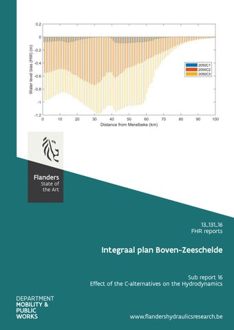
Integraal plan Boven-Zeeschelde Sub report 16 Effect of the C-alternatives on the Hydrodynamics

www.flandershydraulicsresearch.be

Integraal Plan Boven-Zeeschelde Sub report 16 – Effect of the C-alternatives on the Hydrodynamics

Bi, Q.; Vanlede, J.; Smolders, S.; Mostaert, F.

Cover figure © The Government of Flanders, Department of Mobility and Public Works, Flanders Hydraulics Legal notice Flanders Hydraulics Research is of the opinion that the information and positions in this report are substantiated by the available data and knowledge at the time of writing. The positions taken in this report are those of Flanders Hydraulics Research and do not reflect necessarily the opinion of the Government of Flanders or any of its institutions. Flanders Hydraulics Research nor any person or company acting on behalf of Flanders Hydraulics Research is responsible for any loss or damage arising from the use of the information in this report. Copyright and citation © The Government of Flanders, Department of Mobility and Public Works, Flanders Hydraulics Research 2021 D/2021/3241/139 This publication should be cited as follows: Bi, Q.; Vanlede, J.; Smolders, S.; Mostaert, F. (2021). Integraal Plan Boven-Zeeschelde: Sub report 16 – Effect of the Calternatives on the Hydrodynamics. Version 1.0. FHR Reports, 13_131_16. Flanders Hydraulics Research: Antwerp Reproduction of and reference to this publication is authorised provided the source is acknowledged correctly. Document identification Customer: Keywords (3-5): Knowledge domains: Text (p.): Confidential:

IMDC iov dVW-RC Ref.: WL2021R13_131_16 Scaldis model, Scheldt estuary, Hydrodynamics, Telemac Hydraulics and sediment > Hydraulics > Hydrodynamic model > Numerical modelling 60 Appendices (p.): 36 ‫ ܈‬No ‫ ܈‬Available online

Author(s):

Bi, Q.

Control Name Vanlede, J. Reviser(s):

Signature Getekend door:Joris Vanlede (Signature) Getekend door:Sven Smolders (Signature Getekend op:2021-05-07 13:58:29 +02:00 Getekend op:2021-05-06 14:53:43 +02:0 Reden:Ik keur dit document goed Reden:Ik keur dit document goed

Smolders, S.

Project leader:

Vanlede, J.

Getekend door:Joris Vanlede (Signature) Getekend op:2021-05-07 13:59:56 +02:0 Reden:Ik keur dit document goed

Approval Head of Division:

F-WL-PP10-2 Version 7 Valid as from 3/01/2017

Mostaert, F.

Getekend door:Frank Mostaert (Signature Getekend op:2021-05-06 15:19:39 +02:0 Reden:Ik keur dit document goed

Integraal Plan Boven-Zeeschelde - Sub report 16 – Effect of the C-alternatives on the Hydrodynamics

Abstract In the project “Integral Plan for the Upper Sea Scheldt”, a 3D Scaldis-model of the tidal Scheldt estuary is used to analyse the effects of several bathymetry alternatives under different climate scenarios (boundary conditions). This report focuses on the effects of C alternatives on the hydrodynamics under 3 different boundary conditions: A0CN, AminCL and AplusCH. The model results are analysed in terms of water levels, harmonic components, velocities, and tidal asymmetry. The input for the subsequent ecotope analysis (inundation frequency, frequency of the flow velocity that exceeds 0.65 m/s and frequency of the bed shear stress that exceeds 1 Pa) is also presented.

Final version

WL2021R13_131_16

III

F-WL-PP10-2 Version 7 Valid as from 3/01/2017

Integraal Plan Boven-Zeeschelde - Sub report 16 – Effect of the C-alternatives on the Hydrodynamics

Contents Abstract ............................................................................................................................................................ III Contents ............................................................................................................................................................ V List of tables..................................................................................................................................................... VII List of figures .................................................................................................................................................. VIII 1

Introduction ............................................................................................................................................... 1

C-alternatives............................................................................................................................................. 2

2.1

Overview of the measures in C alternatives...................................................................................... 2

2.2

Bathymetry ........................................................................................................................................ 5

Hydrodynamic scenarios ........................................................................................................................... 9 3.1

Normal (QN) and Events (QE) discharge scenarios ........................................................................... 9

3.2

Tidal range scenarios ....................................................................................................................... 12

3.3

Sea level rise scenarios .................................................................................................................... 13

3.4

List of model runs ............................................................................................................................ 13

Methodology of determining HD effect .................................................................................................. 15 4.1

Combination of 4QN+QE run ........................................................................................................... 15

4.2

Harmonic analysis ............................................................................................................................ 15

4.3

Statistical analysis ............................................................................................................................ 15

4.4

Tidal asymmetry .............................................................................................................................. 16

4.4.1

Tidal asymmetry associated with duration ............................................................................. 16

4.4.2 Tidal asymmetry associated with the magnitudes of maximum flood and maximum ebb velocities 17 4.4.3 4.5 5

Interpretation .......................................................................................................................... 19

Ecotope analysis .............................................................................................................................. 19

Results ..................................................................................................................................................... 20 5.1

Reference 2050REF_C...................................................................................................................... 20

5.2

Overview of the effects of C-alternatives........................................................................................ 22

5.3

Effects of C1 ..................................................................................................................................... 23

5.3.1

Effects on water level .............................................................................................................. 24

5.3.2

Effects on cross-sectionally averaged velocity ........................................................................ 28

5.3.3

Effects on tidal asymmetry ...................................................................................................... 31

5.3.4

Input for Ecotope analysis ....................................................................................................... 32

5.4

Effects of C2 ..................................................................................................................................... 35

Final version

WL2021R13_131_16

Integraal Plan Boven-Zeeschelde - Sub report 16 – Effect of the C-alternatives on the Hydrodynamics

5.4.1

Effects on water level .............................................................................................................. 35

5.4.2

Effects on cross-sectionally averaged velocity ........................................................................ 40

5.4.3

Effects on tidal asymmetry ...................................................................................................... 42

5.4.4

Input for ecotope analysis ....................................................................................................... 43

5.5

5.5.1

Effects on water level .............................................................................................................. 46

5.5.2

Effects on cross-sectionally averaged velocity ........................................................................ 51

5.5.3

Effects on tidal asymmetry ...................................................................................................... 53

5.5.4

Input for ecotope analysis ....................................................................................................... 54

5.6 6

Effects of C3 ..................................................................................................................................... 46

Comparison with 1D model ............................................................................................................. 57

Conclusions .............................................................................................................................................. 59

References ....................................................................................................................................................... 60 Appendix 1

Harmonic analysis for C alternatives ...................................................................................... A1

A0CN scenario ............................................................................................................................................. A1 AminCL scenario .......................................................................................................................................... A4 AplusCH scenario ......................................................................................................................................... A7 Appendix 2

Tidal asymmetry for C alternatives ....................................................................................... A10

A0CN scenario ........................................................................................................................................... A10 (1)

Duration asymmetry .................................................................................................................. A10

(2)

Velocity asymmetry ................................................................................................................... A11

AminCL scenario ........................................................................................................................................ A13 (1)

Duration asymmetry .................................................................................................................. A13

(2)

Velocity asymmetry ................................................................................................................... A14

AplusCH scenario ....................................................................................................................................... A16 (1)

Duration asymmetry .................................................................................................................. A16

(2)

Velocity asymmetry ................................................................................................................... A17

Appendix 3

Ecotope analysis (AminCL and AplusCH) .............................................................................. A19

AminCL scenario ........................................................................................................................................ A19 (1)

Inundation frequency ................................................................................................................ A19

(2)

Frequency of velocity magnitude > 0.65 m/s ............................................................................ A22

(3)

Exceedance rate of bed shear stress > 1 Pa .............................................................................. A25

AplusCH scenario ....................................................................................................................................... A28

(1)

Inundation frequency ................................................................................................................ A28

(2)

Frequency of velocity magnitude > 0.65 m/s ............................................................................ A31

(3)

Exceedance rate of bed shear stress > 1 Pa .............................................................................. A34

WL2021R13_131_16

Final version

Integraal Plan Boven-Zeeschelde - Sub report 16 – Effect of the C-alternatives on the Hydrodynamics

List of tables Table 1 – Overview of all measures in the C alternatives ................................................................................. 3 Table 2 – Tidal range scenarios ....................................................................................................................... 12 Table 3 – List of different scenario runs .......................................................................................................... 14

Final version

WL2021R13_131_16

VII

Integraal Plan Boven-Zeeschelde - Sub report 16 – Effect of the C-alternatives on the Hydrodynamics

List of figures Figure 1 – The bathymetry used in the 2050REF_C .......................................................................................... 5 Figure 2 – Bathymetry difference from km24 to km65 (2050C1-2050REF_C) .................................................. 6 Figure 3 – Bathymetry difference from km1 to km23 (2050C1-2050REF_C) .................................................... 6 Figure 4 – Bathymetry difference from km24 to km65 (2050C2-2050REF_C) .................................................. 7 Figure 5 – Bathymetry difference from km1 to km23 (2050C2-2050REF_C) .................................................... 7 Figure 6 – Bathymetry difference from km24 to km65 (2050C3-2050REF_C) .................................................. 8 Figure 7 – Bathymetry difference from km1 to km23 (2050C3-2050REF_C) .................................................... 8 Figure 8 – Synthetic discharge time series for 3 months for the current state (QN2013) ................................ 9 Figure 9 – Synthetic discharge time series for 3 months for 2050 (QN2050) ................................................. 10 Figure 10 – Combination of the time series of QE discharges for the current state (QE2013)....................... 11 Figure 11 – Combination of the time series of QE discharges for 2050 (QE2050) .......................................... 11 Figure 12 – 10-year average tidal range between 1901 and 2010. ................................................................. 12 Figure 13 – Mean water level in the 2050REF_C runs under different climate scenarios .............................. 20 Figure 14 – Water level M2 amplitude (left) and phase (right) under different climate scenarios in 2050REF_C ......................................................................................................................................................................... 21 Figure 15 – Mean cross-sectionally averaged velocity during ebb and flood under different climate scenarios in 2050REF_C ................................................................................................................................................... 21 Figure 16 – Tidal asymmetry (Tflood/Tebb) under different climate scenarios in 2050REF_C ............................ 22 Figure 17 – Effect of the C alternatives on water level under A0CN scenario ................................................ 22 Figure 18 – Effect of the C alternatives on cross-sectionally averaged velocity ............................................. 23 Figure 19 – Effect of 2050C1 on water level M2 amplitude ............................................................................ 24 Figure 20 – Effect of 2050C1 on water level M2 phase................................................................................... 24 Figure 21 – Bathymetry of 2050REF_C and 2050C1 in Km 15-20 ................................................................... 25 Figure 22 – Bathymetry of 2050REF_C and 2050C1 in Km 35-56 ................................................................... 25 Figure 23 – Bathymetry of 2050REF_C and 2050C1 in Km 56-64 ................................................................... 26 Figure 24 – Water level bias based on complete timeseries (2050C1) ........................................................... 27 Figure 25 – Water level bias during HW (2050C1) .......................................................................................... 27 Figure 26 – Water level bias during LW (2050C1) ........................................................................................... 28 Figure 27 – Cross-sectionally averaged velocity bias during ebb (2050C1) .................................................... 28 Figure 28 – Bathymetry of 2050REF_C and 2050C1 in Km 8-10...................................................................... 29 Figure 29 – Bathymetry of 2050REF_C and 2050C1 in Km 12-13 ................................................................... 29 Figure 30 – Cross-sectionally averaged velocity bias during flood (2050C1) .................................................. 30 Figure 31 – Effect of 2050C1 on tidal asymmetry Tflood/Tebb............................................................................ 31

VIII

WL2021R13_131_16

Final version

Integraal Plan Boven-Zeeschelde - Sub report 16 – Effect of the C-alternatives on the Hydrodynamics

Figure 32 – The effect of C1 on the inundation frequency in the Upper Sea Scheldt from km 23-65 (A0CN) 32 Figure 33 – The effect of C1 on the inundation frequency in the Upper Sea Scheldt from km 1-23 (A0CN) . 32 Figure 34 – The effect of C1 on the frequency of velocity magnitude > 0.65 m/s in the Upper Sea Scheldt from km 23-65 (A0CN) ............................................................................................................................................. 33 Figure 35 – The effect of C1 on the frequency of velocity magnitude > 0.65 m/s in the Upper Sea Scheldt from km 1-23 (A0CN) ............................................................................................................................................... 33 Figure 36 – The effect of C1 on the exceedance rate of bed shear stress > 1 Pa in the Upper Sea Scheldt from km 23-65 (A0CN) ............................................................................................................................................. 34 Figure 37 – The effect of C1 on the exceedance rate of bed shear stress > 1 Pa in the Upper Sea Scheldt from km 1-23 (A0CN) ............................................................................................................................................... 34 Figure 38 – Effect of 2050C2 on water level M2 amplitude ............................................................................ 35 Figure 39 – Effect of 2050C2 on water level M2 phase................................................................................... 35 Figure 40 – Bathymetry of 2050REF_C and 2050C2 in Km 1-13...................................................................... 36 Figure 41 – Bathymetry of 2050REF_C and 2050C2 in Km 14-34 ................................................................... 37 Figure 42 – Bathymetry of 2050REF_C and 2050C2 in Km 35-56 ................................................................... 37 Figure 43 – Bathymetry of 2050REF_C and 2050C2 in Km 56-64 ................................................................... 38 Figure 44 – Effect on average water level (2050C2)........................................................................................ 39 Figure 45 – Effect on HW (2050C2) ................................................................................................................. 39 Figure 46 – Effect on LW (2050C2) .................................................................................................................. 40 Figure 47 – Cross-sectionally averaged velocity bias during ebb (2050C2) .................................................... 40 Figure 48 – Cross-sectionally averaged velocity bias during flood (2050C2) .................................................. 41 Figure 49 – Effect of 2050C2 on tidal asymmetry Tflood/Tebb............................................................................ 42 Figure 50 – The effect of C2 on the inundation frequency in the Upper Sea Scheldt from km 23-65 (A0CN) 43 Figure 51 – The effect of C2 on the inundation frequency in the Upper Sea Scheldt from km 1-23 (A0CN) . 43 Figure 52 – The effect of C2 on the frequency of velocity magnitude > 0.65 m/s in the Upper Sea Scheldt from km 23-65 (A0CN) ............................................................................................................................................. 44 Figure 53 – The effect of C2 on the frequency of velocity magnitude > 0.65 m/s in the Upper Sea Scheldt from km 1-23 (A0CN) ............................................................................................................................................... 44 Figure 54 – The effect of C2 on the exceedance rate of bed shear stress > 1 Pa in the Upper Sea Scheldt from km 23-65 (A0CN) ............................................................................................................................................. 45 Figure 55 – The effect of C2 on the exceedance rate of bed shear stress > 1 Pa in the Upper Sea Scheldt from km 1-23 (A0CN) ............................................................................................................................................... 45 Figure 56 – Effect of 2050C3 on water level M2 amplitude ............................................................................ 46 Figure 57 – Effect of 2050C3 on water level M2 phase................................................................................... 46 Figure 58 – Bathymetry of 2050REF_C and 2050C3 in Km 1-13...................................................................... 47 Figure 59 – Bathymetry of 2050REF_C and 2050C3 in Km 14-34 ................................................................... 48 Figure 60 – Bathymetry of 2050REF_C and 2050C3 in Km 35-56 ................................................................... 48 Figure 61 – Bathymetry of 2050REF_C and 2050C3 in Km 56-64 ................................................................... 49 Figure 62 – Water level bias based on complete timeseries (2050C3) ........................................................... 50

Final version

WL2021R13_131_16

Integraal Plan Boven-Zeeschelde - Sub report 16 – Effect of the C-alternatives on the Hydrodynamics

Figure 63 – Water level bias during HW (2050C3) .......................................................................................... 50 Figure 64 – Water level bias during LW (2050C3) ........................................................................................... 51 Figure 65 – Cross-sectionally averaged velocity bias during ebb (2050C3) .................................................... 51 Figure 66 – Cross-sectionally averaged velocity bias during flood (2050C3) .................................................. 52 Figure 67 – Effect of 2050C3 on tidal asymmetry Tflood/Tebb............................................................................ 53 Figure 68 – The effect of C3 on the inundation frequency in the Upper Sea Scheldt from km 23-65 (A0CN) 54 Figure 69 – The effect of C3 on the inundation frequency in the Upper Sea Scheldt from km 1-23 (A0CN) . 54 Figure 70 – The effect of C3 on the frequency of velocity magnitude > 0.65 m/s in the Upper Sea Scheldt from km 23-65 (A0CN) ............................................................................................................................................. 55 Figure 71 – The effect of C3 on the frequency of velocity magnitude > 0.65 m/s in the Upper Sea Scheldt from km 1-23 (A0CN) ............................................................................................................................................... 55 Figure 72 – The effect of C3 on the exceedance rate of bed shear stress > 1 Pa in the Upper Sea Scheldt from km 23-65 (A0CN) ............................................................................................................................................. 56 Figure 73 – The effect of C3 on the exceedance rate of bed shear stress > 1 Pa in the Upper Sea Scheldt from km 1-23 (A0CN) ............................................................................................................................................... 56 Figure 74 – Longitudinal profile of the maximum water levels for REF-2050-C and C1 alternative under T1 storm (Coen et al. 2020) .................................................................................................................................. 57 Figure 75 – Longitudinal profile of the maximum water levels for REF-2050-C and C2 alternative under T1 storm (Coen et al. 2020) .................................................................................................................................. 57 Figure 76 – Longitudinal profile of the maximum water levels for REF-2050-C and C3 alternative under T1 storm (Coen et al. 2020) .................................................................................................................................. 58 Figure 77 – Water level bias in HW from C alternatives (A0CN) ..................................................................... 58 Figure 78 – Water level M2 amplitude (A0CN) ............................................................................................... A1 Figure 79 – Water level M2 phase (A0CN) ...................................................................................................... A1 Figure 80 – Water level M4 amplitude (A0CN) ............................................................................................... A2 Figure 81 – Water level M4 phase (A0CN) ...................................................................................................... A2 Figure 82 – Water level S2 amplitude (A0CN) ................................................................................................. A3 Figure 83 – Water level S2 phase (A0CN) ........................................................................................................ A3 Figure 84 – Water level M2 amplitude (AminCL) ............................................................................................ A4 Figure 85 – Water level M2 phase (AminCL) ................................................................................................... A4 Figure 86 – Water level M4 amplitude (AminCL) ............................................................................................ A5 Figure 87 – Water level M4 phase (AminCL) ................................................................................................... A5 Figure 88 – Water level S2 amplitude (AminCL) .............................................................................................. A6 Figure 89 – Water level S2 phase (AminCL)..................................................................................................... A6 Figure 90 – Water level M2 amplitude (AplusCH) ........................................................................................... A7 Figure 91 – Water level M2 phase (AplusCH) .................................................................................................. A7 Figure 92 – Water level M4 amplitude (AplusCH) ........................................................................................... A8 Figure 93 – Water level M4 phase (AplusCH) .................................................................................................. A8

WL2021R13_131_16

Final version

Integraal Plan Boven-Zeeschelde - Sub report 16 – Effect of the C-alternatives on the Hydrodynamics

Figure 94 – Water level S2 amplitude (AplusCH) ............................................................................................ A9 Figure 95 – Water level S2 phase (AplusCH) ................................................................................................... A9 Figure 96 – Tidal asymmetry Trising/Tfalling (A0CN) ........................................................................................... A10 Figure 97 – Tidal asymmetry Tflood/Tebb (A0CN) .............................................................................................. A10 Figure 98 – Tidal asymmetry Vmeanflood/Vmeanebb (A0CN) ........................................................................... A11 Figure 99 – Tidal asymmetry Vmaxflood/Vmaxebb (A0CN) ............................................................................... A11 Figure 100 – Tidal asymmetry V3flood/V3ebb (A0CN) ....................................................................................... A12 Figure 101 – Tidal asymmetry V4flood/V4ebb (A0CN) ....................................................................................... A12 Figure 102 – Tidal asymmetry Trising/Tfalling (AminCL) ...................................................................................... A13 Figure 103 – Tidal asymmetry Tflood/Tebb (AminCL) ........................................................................................ A13 Figure 104 – Tidal asymmetry Vmeanflood/Vmeanebb (AminCL) ..................................................................... A14 Figure 105 – Tidal asymmetry Vmaxflood/Vmaxebb (AminCL) .......................................................................... A14 Figure 106 – Tidal asymmetry V3flood/V3ebb (AminCL) .................................................................................... A15 Figure 107 – Tidal asymmetry V4flood/V4ebb (AminCL) .................................................................................... A15 Figure 108 – Tidal asymmetry Trising/Tfalling (AplusCH)..................................................................................... A16 Figure 109 – Tidal asymmetry Tflood/Tebb (AplusCH) ....................................................................................... A16 Figure 110 – Tidal asymmetry Vmeanflood/Vmeanebb (AplusCH) .................................................................... A17 Figure 111 – Tidal asymmetry Vmaxflood/Vmaxebb (AplusCH) ......................................................................... A17 Figure 112 – Tidal asymmetry V3flood/V3ebb (AplusCH) .................................................................................. A18 Figure 113 – Tidal asymmetry V4flood/V4ebb (AplusCH) .................................................................................. A18 Figure 114 – The effect of C1 on the inundation frequency in the Upper Sea Scheldt from km 23-65 (AminCL) ....................................................................................................................................................................... A19 Figure 115 – The effect of C1 on the inundation frequency in the Upper Sea Scheldt from km 1-23 (AminCL) ....................................................................................................................................................................... A19 Figure 116 – The effect of C2 on the inundation frequency in the Upper Sea Scheldt from km 23-65 (AminCL) ....................................................................................................................................................................... A20 Figure 117 – The effect of C2 on the inundation frequency in the Upper Sea Scheldt from km 1-23 (AminCL) ....................................................................................................................................................................... A20 Figure 118 – The effect of C3 on the inundation frequency in the Upper Sea Scheldt from km 23-65 (AminCL) ....................................................................................................................................................................... A21 Figure 119 – The effect of C3 on the inundation frequency in the Upper Sea Scheldt from km 1-23 (AminCL) ....................................................................................................................................................................... A21 Figure 120 – The effect of C1 on the frequency of velocity magnitude > 0.65 m/s in the Upper Sea Scheldt from km 23-65 (AminCL) ............................................................................................................................... A22 Figure 121 – The effect of C1 on the frequency of velocity magnitude > 0.65 m/s in the Upper Sea Scheldt from km 1-23 (AminCL) ................................................................................................................................. A22 Figure 122 – The effect of C2 on the frequency of velocity magnitude > 0.65 m/s in the Upper Sea Scheldt from km 23-65 (AminCL) ............................................................................................................................... A23

Final version

WL2021R13_131_16

Integraal Plan Boven-Zeeschelde - Sub report 16 – Effect of the C-alternatives on the Hydrodynamics

Figure 123 – The effect of C2 on the frequency of velocity magnitude > 0.65 m/s in the Upper Sea Scheldt from km 1-23 (AminCL) ................................................................................................................................. A23 Figure 124 – The effect of C3 on the frequency of velocity magnitude > 0.65 m/s in the Upper Sea Scheldt from km 23-65 (AminCL) ............................................................................................................................... A24 Figure 125 – The effect of C3 on the frequency of velocity magnitude > 0.65 m/s in the Upper Sea Scheldt from km 1-23 (AminCL) ................................................................................................................................. A24 Figure 126 – The effect of C1 on the exceedance rate of bed shear stress > 1 Pa in the Upper Sea Scheldt from km 23-65 (AminCL) ........................................................................................................................................ A25 Figure 127 – The effect of C1 on the exceedance rate of bed shear stress > 1 Pa in the Upper Sea Scheldt from km 1-23 (AminCL) .......................................................................................................................................... A25 Figure 128 – The effect of C2 on the exceedance rate of bed shear stress > 1 Pa in the Upper Sea Scheldt from km 23-65 (AminCL) ........................................................................................................................................ A26 Figure 129 – The effect of C2 on the exceedance rate of bed shear stress > 1 Pa in the Upper Sea Scheldt from km 1-23 (AminCL) .......................................................................................................................................... A26 Figure 130 – The effect of C3 on the exceedance rate of bed shear stress > 1 Pa in the Upper Sea Scheldt from km 23-65 (AminCL) ........................................................................................................................................ A27 Figure 131 – The effect of C3 on the exceedance rate of bed shear stress > 1 Pa in the Upper Sea Scheldt from km 1-23 (AminCL) .......................................................................................................................................... A27 Figure 132 – The effect of C1 on the inundation frequency in the Upper Sea Scheldt from km 23-65 (AplusCH) ....................................................................................................................................................................... A28 Figure 133 – The effect of C1 on the inundation frequency in the Upper Sea Scheldt from km 1-23 (AplusCH) ....................................................................................................................................................................... A28 Figure 134 – The effect of C2 on the inundation frequency in the Upper Sea Scheldt from km 23-65 (AplusCH) ....................................................................................................................................................................... A29 Figure 135 – The effect of C2 on the inundation frequency in the Upper Sea Scheldt from km 1-23 (AplusCH) ....................................................................................................................................................................... A29 Figure 136 – The effect of C3 on the inundation frequency in the Upper Sea Scheldt from km 23-65 (AplusCH) ....................................................................................................................................................................... A30 Figure 137 – The effect of C3 on the inundation frequency in the Upper Sea Scheldt from km 1-23 (AplusCH) ....................................................................................................................................................................... A30 Figure 138 – The effect of C1 on the frequency of velocity magnitude > 0.65 m/s in the Upper Sea Scheldt from km 23-65 (AplusCH) .............................................................................................................................. A31 Figure 139 – The effect of C1 on the frequency of velocity magnitude > 0.65 m/s in the Upper Sea Scheldt from km 1-23 (AplusCH) ................................................................................................................................ A31 Figure 140 – The effect of C2 on the frequency of velocity magnitude > 0.65 m/s in the Upper Sea Scheldt from km 23-65 (AplusCH) .............................................................................................................................. A32 Figure 141 – The effect of C2 on the frequency of velocity magnitude > 0.65 m/s in the Upper Sea Scheldt from km 1-23 (AplusCH) ................................................................................................................................ A32 Figure 142 – The effect of C3 on the frequency of velocity magnitude > 0.65 m/s in the Upper Sea Scheldt from km 23-65 (AplusCH) .............................................................................................................................. A33 Figure 143 – The effect of C3 on the frequency of velocity magnitude > 0.65 m/s in the Upper Sea Scheldt from km 1-23 (AplusCH) ................................................................................................................................ A33

XII

WL2021R13_131_16

Final version

Integraal Plan Boven-Zeeschelde - Sub report 16 – Effect of the C-alternatives on the Hydrodynamics

Figure 144 – The effect of C1 on the exceedance rate of bed shear stress > 1 Pa in the Upper Sea Scheldt from km 23-65 (AplusCH) ....................................................................................................................................... A34 Figure 145 – The effect of C1 on the exceedance rate of bed shear stress > 1 Pa in the Upper Sea Scheldt from km 1-23 (AplusCH) ......................................................................................................................................... A34 Figure 146 – The effect of C2 on the exceedance rate of bed shear stress > 1 Pa in the Upper Sea Scheldt from km 23-65 (AplusCH) ....................................................................................................................................... A35 Figure 147 – The effect of C2 on the exceedance rate of bed shear stress > 1 Pa in the Upper Sea Scheldt from km 1-23 (AplusCH) ......................................................................................................................................... A35 Figure 148 – The effect of C3 on the exceedance rate of bed shear stress > 1 Pa in the Upper Sea Scheldt from km 23-65 (AplusCH) ....................................................................................................................................... A36 Figure 149 – The effect of C3 on the exceedance rate of bed shear stress > 1 Pa in the Upper Sea Scheldt from km 1-23 (AplusCH) ......................................................................................................................................... A36

Final version

WL2021R13_131_16

XIII

Integraal Plan Boven-Zeeschelde - Sub report 16 – Effect of the C-alternatives on the Hydrodynamics

1 Introduction This reports focuses on the analysis of the effects of the C alternatives on the hydrodynamics in the Upper Sea Scheldt. Time is expressed in CET (Central European Time). Depth, height, and water levels are expressed in meter, TAW (Tweede Algemene Waterpassing). Bathymetry and water levels are positive above the reference plane. The coordinate system is RD Paris. Distance along the estuary is measured from the lock in Merelbeke

Final version

WL2021R13_131_16

Integraal Plan Boven-Zeeschelde - Sub report 16 – Effect of the C-alternatives on the Hydrodynamics

2 C-alternatives The definition of the C alternatives has three variations, which have been described in detail in the memo ‘Definition of C alternatives’ (IMDC, 2021) which has been discussed with international experts (EGIPUS) in a workshop 18th June 2019. Overview of the measures and bathymetries of the C alternatives is discussed below.

2.1 Overview of the measures in C alternatives A gradual approach is taken in building up the C alternatives in order to fully understand the extent, to which measures of a certain scale respond (IMDC, 2021). Generally, in the C alternatives, different focuses are put between the up and downstream section. For the upstream, it is important to improve the riverine and safety functions, while for the downstream, it becomes crucial to improve the estuarine functions. The three alternatives are developed with the following mindset: •

C1 alternative: Tackle the most prominent nautical bottlenecks (Km 0 – Ringvaart, km 10 – Wetteren, km 15 till 17 – Hoogland and Uitbergen, Km 30 – Kasteeltje, km 40 – Kramp). Looking for opportunities in the river and redefining the Sigma plan to improve habitat and to reduce the increase in tidal amplitude (from climate change and due to nautical changes).

•

C2 alternative: Tackle also less prominent nautical bottlenecks and define additional measures for the most prominent bottlenecks. Include additional opportunities in the valley (depolderings, side channels) to improve habitat and reduce increase in tidal amplitude.

•

C3 alternative: Yet additional nautical measures for a limited number of locations (Uitbergen, Paardenweide, Kasteeltje) and additional measures (larger derpolderings, additional depoldering at Weert, undeepening at Temse) aiming at providing extra resilience while also improving habitat conditions.

All the C alternatives are designed based on the sustainable bathymetry for 2050 (IMDC, 2015). In general, there are three types of measures incorporated in the design: •

Adaptations to the navigation channel;

•

Adaptations to the channel bathymetry to allow for intertidal nature development;

•

Definition of additional areas in the valley (depoldering, CRT, FCA).

The overview of the implemented measures is presented in Table 1.

WL2021R13_131_16

Final version

Integraal Plan Boven-Zeeschelde - Sub report 16 – Effect of the C-alternatives on the Hydrodynamics Table 1 – Overview of all measures in the C alternatives (IMDC, 2021)

Distance to Merelbeke [km]

Overview measures C1

MHW

MLW

[m TAW]

5.05

2.44

5.05

2.44

5.05

2.44

5.06

2.37

5.07

2.28

5.08

2.23

Depoldering

5.08

2.23

Additional FCA in the north

5.08

2.12

5.10

2.10

5.10

2.02

Ringvaart

0-3

Veerhoek

4.5

Melleham

5.5

Limited tidal interaction

Bommels

6.5

Voorde

Wetteren

DS Wetteren

12.5

FCA Wijmeers

Wijmeers (Hoogland)

Uitbergen

Paardenweide (Wichelen)

Bend cut off+depoldering

5.10

1.95

Oude Broekmeer

24-27

Depoldering variant 1 + side channel

Depoldering variant 2 + side channel

5.17

1.63

Appels (Scheldebroek)

Improved navigation by smoothing the bend (cfr Chafing)

5.20

1.50

Scheldebroek

FCA Scheldebroek converted into FCA-CRT

5.20

1.50

Sint-Onolfspolder

28-30

5.20

1.50

Kasteeltje

5.27

1.24

Dender

32.5

Improved navigation by widening channel

5.3

1.12

Grembergen broek – Armenput

35-38

Depoldering

5.34

1.02

Waterleiding

5.38

0.91

Roggeman

5.40

0.85

Final version

Deepening and widening (also present in 2050REF_C) Widening + pull back of dyke CRT without FCA

Depoldering

Widening + pull back of dyke Bend modifications + intertidal nature

Improved navigation (cfr VaG) by installing sheet piles

Bend cut off (C1: variant 1, C2: variant 2, C3: variant 3) + intertidal nature+FCA Bend cut off + intertidal nature+depoldering (C1: variant 1, C2: variant 2, C3: variant 3)

Depoldering variant 1 + side channel variant 1

Depoldering variant 1 + side channel variant 2

Bend smoothening + intertidal nature (C1: variant 1, C2: variant 2, C3: variant 3)

Improved navigation (cfr Chafing) by widening channel -

Depoldering variant 1

WL2021R13_131_16

Depoldering variant 2

Integraal Plan Boven-Zeeschelde - Sub report 16 – Effect of the C-alternatives on the Hydrodynamics

Distance to Merelbeke [km]

Overview measures C1

Bend cut off + intertidal nature (C1: variant 1; C2-C3: variant 2)

MHW

MLW

[m TAW]

5.44

0.75

Kockham (Kramp)

Wal-Zwijn

44-48

FCA-CRT

5.50

0.59

Blankaart

FCA

Depoldering variant 1

Depoldering variant 2

5.55

0.40

Akkershoofd

Depoldering together with Blankaart

5.54

0.38

Tielrode Broek

New connection with Durme + partly depoldering Tielrode Broek

5.52

0.31

Weert

51-56

Depoldering

5.52

0.31

Temse to Rupel

57-64

Local fill-in + reducing channel depth

5.46

0.15

Schouselbroek

Depoldering + new side channel

5.47

0.19

Schellandpolder

Depoldering + new side channel

5.47

0.16

Oudbroekpolder

Depoldering + new side channel

5.45

0.13

Spierbroekpolder and Hingene Broekpolder

60-64

Local fill-in

activated as FCA-CRT

WL2021R13_131_16

Final version

Integraal Plan Boven-Zeeschelde - Sub report 16 – Effect of the C-alternatives on the Hydrodynamics

2.2 Bathymetry For implementing the three different C alternatives (C1, C2 and C3) in the SCALDIS model, a new reference grid is created based on the original 2050REF grid used in the B-alternatives (2050REF_B). This new reference grid, named 2050REF_C, is then used as the basis for implementing the C alternatives. Figure 1 – The bathymetry used in the 2050REF_C

The new reference grid is obtained by extending and refining the 2050REF_B mesh in the Upper Sea Scheldt in order to include the maximum outline of all C alternatives. For the rest of the domain except in the Ringvaart (a widened and deepend Ringvaart is applied to the 2050REF_C and all the C alternatives later), the grid remains unmodified, in order to allow the reuse of the boundary data. In the extended areas in the Upper Sea Scheldt, the finest grid resolution is about 7 m, and the coarsest resolution is about 50 m. The new reference grid is able to accommodate the adaptations of the navigation channel, the new development of intertidal nature and the additional de-embankments and FCAs (with and without CRT), which are considered in any of the C alternatives. The sustainable bathymetry in the 2050REF_B grid with the deepening and widening of the Ringvaart is mapped to the new reference grid 2050REF_C, except for the newly extended areas. For the extended areas, the background bathymetry without any modification from the C alternatives (provided by IMDC) is used as the data source. The background bathymetry does not contain any measure for 2050, it represents the current situation. When incorporating the C alternatives, the new bathymetry from C1, C2 and C3 is mapped to the 2050REF_C grid, respectively. The implementation of C alternatives is described in detail in Bi et al. (2020). The difference of bathymetry between the C alternatives and 2050REF_C are shown in Figure 2 to Figure 7 as an overview of the locations of the new measures. The actual bathymetry of C1, C2 and C3 will be discussed in Chapter 5.

Final version

WL2021R13_131_16

Integraal Plan Boven-Zeeschelde - Sub report 16 – Effect of the C-alternatives on the Hydrodynamics Figure 2 – Bathymetry difference from km24 to km65 (2050C1-2050REF_C) (Purple means the new bathymetry of 2050C1 is deeper than the reference bathymetry, and brown means higher)

Figure 3 – Bathymetry difference from km1 to km23 (2050C1-2050REF_C) (Purple means the new bathymetry of 2050C1 is deeper than the reference bathymetry, and brown means higher)

WL2021R13_131_16

Final version

Integraal Plan Boven-Zeeschelde - Sub report 16 – Effect of the C-alternatives on the Hydrodynamics Figure 4 – Bathymetry difference from km24 to km65 (2050C2-2050REF_C) (Purple means the new bathymetry of 2050C1 is deeper than the reference bathymetry, and brown means higher)

Figure 5 – Bathymetry difference from km1 to km23 (2050C2-2050REF_C) (Purple means the new bathymetry of 2050C1 is deeper than the reference bathymetry, and brown means higher)

Final version

WL2021R13_131_16

Integraal Plan Boven-Zeeschelde - Sub report 16 – Effect of the C-alternatives on the Hydrodynamics Figure 6 – Bathymetry difference from km24 to km65 (2050C3-2050REF_C) (Purple means the new bathymetry of 2050C1 is deeper than the reference bathymetry, and brown means higher)

Figure 7 – Bathymetry difference from km1 to km23 (2050C3-2050REF_C) (Purple means the new bathymetry of 2050C1 is deeper than the reference bathymetry, and brown means higher)

The difference of bathymetry between C alternatives and 2050REF_C will be used in the interpretation of the effects on the hydrodynamics in the Upper Sea Scheldt.

WL2021R13_131_16

Final version

Integraal Plan Boven-Zeeschelde - Sub report 16 – Effect of the C-alternatives on the Hydrodynamics

3 Hydrodynamic scenarios The 3D Scaldis-model is used to evaluate the effects of different alternatives (specified bathymetry), under different scenarios (a range of boundary conditions to take into account climate change, sea level rise, increasing or decreasing tidal amplitude and high or low river discharge). The resulting list of the scenario runs is presented in Table 3.

3.1 Normal (QN) and Events (QE) discharge scenarios For the ecotope mapping, water level frequencies distributed over a year are required. The limitations on the calculation time (or cost) of the 3D hydrodynamic model forces the use of a different approach than calculating with very long time series. The bulk of the distribution will be obtained by running the hydrodynamic model for a period of 3 months with a synthetic discharge boundary containing events with a return period equal to or smaller than ¼ year. This is the “normal” discharge scenario (QN). The downstream (tidal) boundary is a harmonic boundary without storm surge. The upstream boundary is a synthetic discharge boundary containing events with a return period equal to or smaller than 1/6 year (combined with QE (T1 & T1/2) this results in 6 exceedances of this discharge). The simulation period is 3 months. The QN discharges for the current state (QN2013) is applied to the runs for the current situation. The QN discharge for the 2050 (QN2050) is used in the rest of the runs for the 2050 situation. A0CN is combined with QN2013, while AminCL and AplusCH is combined with QN2050. Figure 8 – Synthetic discharge time series for 3 months for the current state (QN2013)

Final version

WL2021R13_131_16

Integraal Plan Boven-Zeeschelde - Sub report 16 – Effect of the C-alternatives on the Hydrodynamics Figure 9 – Synthetic discharge time series for 3 months for 2050 (QN2050)

Separately, a run of ca. 2 weeks will be run with a discharge timeseries that contains 3 discharge events with return periods of 1 year, ½ year and 1/3 year. Simultaneously, the downward boundary contains a storm surge period that is added to the harmonic signal. The surge was determined by IMDC in a statistical similar way as the precipitation signal, based on measurements of the last +/-40 years (Vlissingen). This is the “events” (QE) discharge scenario. The upstream boundary is a discharge time series that contains 2 discharge events with return periods of 1 year and 1/2 year. The simulation period is 20 days. Similarly, the QE discharges for the current state (QN2013) is applied to the runs for the current situation, while the QE discharge for the 2050 (QN2050) is used in the rest of the runs for the 2050 situation.

WL2021R13_131_16

Final version

Integraal Plan Boven-Zeeschelde - Sub report 16 – Effect of the C-alternatives on the Hydrodynamics Figure 10 – Combination of the time series of QE discharges for the current state (QE2013)

Figure 11 – Combination of the time series of QE discharges for 2050 (QE2050)

The water level distribution in specific points is obtained by adding the 4 x “normal” and 1 x “events” waterlevel scenarios. The statistical techniques used to determine QN and QE boundary conditions for the 2050 situation are described in IMDC (2015). The implementation of the timeseries described in IMDC (2015) into the boundary conditions for Scaldis is described in chapter 6 of the Scaldis 2050 report (Smolders et al., 2017).

Final version

WL2021R13_131_16

Integraal Plan Boven-Zeeschelde - Sub report 16 – Effect of the C-alternatives on the Hydrodynamics

3.2 Tidal range scenarios The effects of changing the bathymetry of the Upper Sea Scheldt in the C-alternatives are evaluated in a range of boundary conditions (the scenarios). To include possible effects of amplitude changes due to unknown developments outside (downstream) the study areas, a range of tidal amplitudes is considered. The tidal range in the estuary has increased, and the tidal range maximum has moved upwards in the past decades. Figure 12 – 10-year average tidal range between 1901 and 2010. (Kuijper, 2013)

Three different tidal range scenarios A+, A0 and A- have been modeled. In these scenarios, the tidal amplitude at Schelle is equal to 5.70, 5.40 and 5.00 m, respectively, as shown in Table 2. Table 2 – Tidal range scenarios

Scenario

Tidal amplitude at Schelle (m)

A+

5.70

5.40 (current tidal range)

A-

5.00

The increase and decrease of the amplitude is enforced by changing the roughness in the Western Scheldt. By changing the roughness, the tidal propagation is influenced, without simulating specific measures in the downstream parts of the estuary (e.g. creating additional flooding areas, deepening, etc.)

WL2021R13_131_16

Final version

Integraal Plan Boven-Zeeschelde - Sub report 16 – Effect of the C-alternatives on the Hydrodynamics

3.3 Sea level rise scenarios In KNMI (2014), climate scenarios for the Netherlands have been published for the climate around 2050 and 2085, for four climate change scenarios. The four scenarios are the combination of two extremes in global temperature rise (‘moderate’ M and ‘warm’ W) and the two possible atmospheric circulation pattern changes (‘low’ L and ‘high’ H). The combinations lead to scenarios indicated as WL, WH, GL and GH. The climate prediction fork used in the present study could be approached as the extreme values in the four KNMI (2014) scenarios for Sea level rise in the North Sea coast in 2050: •

Scenarios GL, GH; + 15 cm till + 30 cm (90% conf. int.)

•

Scenarios WL, WH; + 20 cm till + 40 cm (90% conf. int.)

The following sea level rise (SLR) scenarios are modelled for 2050: -

No sea level rise (CN, +0 cm in 2050);

The “low” scenario (CL, +15 cm in 2050);

The “high” scenario (CH, +40 cm in 2050).

The downstream boundary conditions for year 2050 are increased with these values. The tidal range scenario A+ is combined with the sea level rise CH. The tidal range scenario A- is combined with the sea level rise CL. The current tidal range condition A0 is combined with zero sea level rise scenario CN. Note that the CH and CL SLR scenarios are calculated in a bathymetry that is based on the current bathymetry. No morphological modelling is done. This implies that the intertidal areas become flooded under these boundary conditions, which impacts the hydrodynamics. In reality, there would be a morphological response of the system to SLR scenarios. The HD results shown here correspond to the so-called “initial response” of the system and should be interpreted with care.

3.4 List of model runs The overview of model runs is presented in Table 3. This table gives the various conditions of each model run, which includes the bathymetry alternative, discharge type, tidal amplitude and sea level rise scenario. The last column shows the duration of each run in days. QN: normal discharge scenario. QE: events discharge scenario. (A0, A+, A-): Different tidal range scenarios. (CN, CL, CH): Sea level rise scenarios. QN runs have a simulation period from 09/08/2050 22:20:00 to 12/11/2050 21:20:00 (95 days). The spin up period is 2 days from 09/08/2050 22:20:00 to 11/08/2050 22:20:00. QE runs have a simulation period from 28/08/2050 11:00 to 17/09/2050 16:00 (20 days). The spin up period is 3 days from 28/08/2050 11:00 to 31/08/2050 11:00.

Final version

WL2021R13_131_16

Integraal Plan Boven-Zeeschelde - Sub report 16 – Effect of the C-alternatives on the Hydrodynamics Table 3 – List of different scenario runs

Code

Year

Bathymetry Discharge Amplitude Sea level (alternatives) correction scenario type

2050REF_C_QN_A0CN

QN2013

2050REF_C_QE_A0CN

QE2013

2050REF_C_QN_AminCL 2050REF_C_QE_AminCL

2050

REF_C

QN2050 QE2050

2050REF_C_QN_AplusCH

QN2050

2050REF_C_QE_AplusCH

QE2050

2050C1_QN_A0CN

QN2013

2050C1_QE_A0CN

QE2013

2050C1_QN_AminCL 2050C1_QE_AminCL

2050

QN2050 QE2050

2050C1_QN_AplusCH

QN2050

2050C1_QE_AplusCH

QE2050

2050C2_QN_A0CN

QN2013

2050C2_QE_A0CN

QE2013

2050C2_QN_AminCL 2050C2_QE_AminCL

2050

QN2050 QE2050

2050C2_QN_AplusCH

QN2050

2050C2_QE_AplusCH

QE2050

2050C3_QN_A0CN

QN2013

2050C3_QE_A0CN

QE2013

2050C3_QN_AminCL 2050C3_QE_AminCL

2050

QN2050 QE2050

2050C3_QN_AplusCH

QN2050

2050C3_QE_AplusCH

QE2050

WL2021R13_131_16

A-

A+

A-

A+

A-

A+

A-

A+

Duration of run [days] 95 20 95 20 95 20 95 20 95 20 95 20 95 20 95 20 95 20 95 20 95 20 95 20

Final version

Integraal Plan Boven-Zeeschelde - Sub report 16 – Effect of the C-alternatives on the Hydrodynamics

4 Methodology of determining HD effect The model results of the three C alternatives (C1, C2, and C3) are presented in Chapter 5. The methodology to determine the hydrodynamic effects is described in this chapter. Because there are three climate scenarios, i.e. A0CN, AminCL and AplusCH, when deriving the effcts, the C alternative runs are only compared with their reference runs under the same climate scenario. The used parameters include water levels, cross-sectionally averaged velocity, harmonic components, biases and tidal asymmetry indicators. Effects are quantified at various locations along the estuary.

4.1 Combination of 4QN+QE run The combination of 4 x “normal” (QN) and 1 x “events” (QE) discharge scenario produces an output for water levels, flow velocities and discharges that is statistically representative for one year. It is worth to mention that the combination of 4QN+QE runs as a synthetic year is not suitable for harmonic analysis. It works well for ecotope analysis, but makes little sense for performing an harmonic analysis on this synthetic timeseries. The synthetic time series is not a continuous sine signal anymore, therefore, classic harmonic analysis fails. Thus, the “normal” discharge scenario (QN) runs are used for the harmonic analysis since their simulation period is the longest, and best suited to obtain harmonic components while 4QN+QE runs are used for ecotope analysis only. In order to relate the changes of harmonic components to other statistical parameters and tidal asymmetry indicators, QN runs are also used for the latter two analyses.

4.2 Harmonic analysis The time series of water level at various locations along the thalweg of the main channel are extracted from the results for each run. At each location, the water levels and cross-sectionally averaged velocities are then decomposed into M2, M4 and S2 signals through harmonic analysis. The obtained water level amplitudes could reveal the change of tidal range due to local measures.

4.3 Statistical analysis The effects of each alternative on the flow hydrodynamics are quantified by the bias in high water, low water and complete time series of water levels and cross-sectionally averaged velocity. The time series of water levels (noted as 𝜁𝜁) are taken from the thalweg points along the Scheldt. The cross-sectionally averaged velocity is derived at transects along the main channel. For each transect, the depth-averaged velocity 𝑢𝑢 is firstly projected on the normal vector 𝒏𝒏 of this transect: 𝑢𝑢�(𝑡𝑡, 𝑠𝑠) = 𝑢𝑢(𝑡𝑡, 𝑥𝑥, 𝑦𝑦) ∙ 𝒏𝒏

Then the cross-sectionally averaged velocity at this transect is: 𝐿𝐿

𝑄𝑄(𝑡𝑡) ∫0 𝑢𝑢�(𝑡𝑡, 𝑠𝑠)ℎ(𝑡𝑡, 𝑠𝑠)𝑑𝑑𝑑𝑑 𝑢𝑢�(𝑡𝑡) = = 𝐿𝐿 𝐴𝐴(𝑡𝑡) ∫0 ℎ(𝑡𝑡, 𝑠𝑠)𝑑𝑑𝑠𝑠

where, 𝑡𝑡 is time, 𝑥𝑥, 𝑦𝑦 are the Cartesian coordinates, 𝒏𝒏 is the normal vector of the transect, 𝑠𝑠 is the coordinate on the transect, ℎ is the water depth, 𝐿𝐿 is the total length of the transect. Final version

WL2021R13_131_16

Integraal Plan Boven-Zeeschelde - Sub report 16 – Effect of the C-alternatives on the Hydrodynamics

The statistical parameters introduced in the report show the differences between bathymetry alternatives and the reference one. Definitions of the used statistical parameters are described as follows: The reference time series is presented as 𝑥𝑥 (𝑥𝑥 = 𝜁𝜁 𝑜𝑜𝑜𝑜 𝑢𝑢�) and the time series that is subject to the test as 𝑦𝑦.

The mean values of the time series are represented by 𝑥𝑥 (reference) and 𝑦𝑦 (subject to test). 𝑁𝑁

1 𝑥𝑥 = � 𝑥𝑥𝑖𝑖 , 𝑁𝑁

where 𝑁𝑁 is the length of the time series.

𝑖𝑖=1

𝑁𝑁

1 𝑦𝑦 = � 𝑦𝑦𝑖𝑖 , 𝑁𝑁 𝑖𝑖=1

The bias is the difference between the mean of the tested and the reference time series,

4.4 Tidal asymmetry

𝑏𝑏𝑏𝑏𝑏𝑏𝑏𝑏 = 𝑦𝑦 − 𝑥𝑥.

Hydrodynamic processes (tides, wind waves, density driven currents and wind induced currents) drive sediment transports and steer morphological developments. Various studies describe tide residual currents in estuaries resulting from tidal asymmetries (Steijn & Van der Spek, 2005; Van der Werf & Brière, 2013; Tonnon & van der Werf, 2014) which are partly confirmed by measured bed forms (Erkens, 2003). Tidal asymmetry is an important parameter for predicting and understanding sediment transport behavior in an estuary, due to the non-linear relation between flow velocity and sediment transport (Van de Kreeke and Robaczewska, 1993; Wang et al., 1999). An estuary (or a part of it) is called ebb dominant or flood dominant depending on the direction of asymmetry. It is possibly a principal factor influencing the sediment exchange between the ebb tidal delta and the estuary, as well as between the various parts of the estuary (Wang et al., 1999; Friedrichs, 2011). The asymmetry of the vertical tide is often described by the difference or ratio between the duration of rising tide (flood) and falling tide (ebb). Similarly, horizontal tidal asymmetry is flood-dominant if the flood flow is stronger, while horizontal asymmetry is ebb dominant if the ebb flow is stronger. Furthermore, the difference in duration of the slack water periods after high and low tide is another indicator for horizontal tidal asymmetry as the deposition of fine (suspended) sediment is closely related to the settling time of particles (e.g. Dronkers, 1986). Finally, tidal asymmetry can also be characterized by the relative contribution of different tidal constituents to the tidal signal, as the amplitude ratios and phase differences between the principal constituents and their overtides or compound tides are indicators for the strength and nature of the tidal asymmetry (e.g. Friedrichs and Aubrey, 1988; Parker, 1984; Wang et al., 1999, 2002). There are clearly many ways of quantifying asymmetry. In the present study, five different ratios for tidal asymmetry are used. The first two parameters are related to duration and the last three are related to current velocities. All ratios are calculated in such a way that >1 is flood dominant, and <1 is ebb dominant. Note that an ebb dominance in duration, will be a flood dominance in velocities, because there is an inverse relation between both. 4.4.1

Tidal asymmetry associated with duration

Tidal duration asymmetry (the difference in the duration and/or amplitude of rising and falling tide) can arise from distortion of the tide in shallow water or from the interaction of astronomical tidal constituents (Parker, 1991). Physically, the crest of the tidal wave (High Water) propagates faster than the trough (Low Water), so within the embayment there is a shorter period of rising water (from LW to HW) than falling tide. HW

WL2021R13_131_16

Final version

Integraal Plan Boven-Zeeschelde - Sub report 16 – Effect of the C-alternatives on the Hydrodynamics

propagation may be slowed if the intertidal volume of adjacent shoals is large relative to channel volume, resulting in a longer period of rising water (Fortunato and Oliveira, 2005). Velocity skew is the asymmetrical distribution of ebb and flood tidal flow over a tidal cycle. This skew can be a local phenomenon caused by bathymetry, as in the case of water flow around a headland, or in channels with segregated flood/ebb conduits (van Veen et al., 2005). On a system-wide scale, shoaling bathymetry contributes to skewed velocities through the distortion of the surface tide, which results in differences between the duration of rising and falling water (Boon and Byrne, 1981). Based on the tidal duration two different asymmetry parameters are used to analyse and to evaluate the effects of each bathymetry alternative. These two parameters are described as follows: Tidal asymmetry of the duration (time) of rising and falling tide: 𝑇𝑇rising 𝑇𝑇falling

Trising = time required within the tidal cycle to change water level from LW to HW; Tfalling = time required within the tidal cycle to change water level from HW to LW. This parameter indicates the relative relation between the duration of rising and falling tide during a full tidal cycle. This ratio gives an indication of the shape of the tidal cycle. This parameter can be different at various locations along the estuary, based on the hydrodynamic conditions at each location. It is important to mention that this parameter has no relation to the duration of the two phases (flood and ebb) of the tidal cycle. Tidal asymmetry based on duration of flood-period and ebb-period : 𝑇𝑇flood 𝑇𝑇ebb

Tflood =

duration of flood flow during the tidal cycle;

Tebb =

duration of ebb flow during the tidal cycle.

This parameter quantifies tidal asymmetry based on the horizontal tide (velocities). It is important to note that this parameter has no direct connection with the previous parameter which is related to asymmetry of the vertical tide. 4.4.2

Tidal asymmetry associated with the magnitudes of maximum flood and maximum ebb velocities

The above two tidal asymmetry parameters are based on tidal variations of water levels (vertical tide) and not the current velocities (horizontal tide), while the sediment transport is linked to the currents. The following three forms of the tidal asymmetry, which have been used in the present study, are based on the current flow velocities.

Final version

WL2021R13_131_16

Integraal Plan Boven-Zeeschelde - Sub report 16 – Effect of the C-alternatives on the Hydrodynamics

Tidal asymmetry of the maximum current flow velocities during flood and ebb phases: One way to look at tidal asymmetry is to look at the difference in peak flood/ebb shear stresses (Dronkers, 1986; Friedrichs and Aubrey, 1988). This type of asymmetry is associated with a difference in the magnitude between maximum flood and ebb velocities. For example, if the maximum flood velocity exceeds the ebb velocity, a residual sediment transport in flood direction is likely to occur, and vice versa. This tidal asymmetry parameter is based on maximum velocity during flood and maximum velocity during ebb within the tidal cycle. Averaged cross-sectionally averaged velocities are computed by dividing the discharge at a certain cross-section by the wet area of this cross-section (V= Discharge (Q) / wet area (A)). 𝑉𝑉max 𝑓𝑓𝑓𝑓𝑓𝑓𝑓𝑓𝑓𝑓 𝑉𝑉max 𝑒𝑒𝑒𝑒𝑒𝑒

Vmaxflood =

maximum cross-sectionally averaged velocity during flood phase;

Vmaxebb =

maximum cross-sectionally averaged velocity during ebb phase.

Tidal asymmetry calculated based on the velocity as proxy for the transport of fine sediments (~𝑽𝑽𝟒𝟒 )

The horizontal sediment flux of mud is assumed to scale with the product of the saturation condition and the flow velocity, i.e. with V4 (e.g. Winterwerp, 2001). According to Winterwerp (2001), when the flow velocity decreases slightly, sediment (mud) starts to settle, creating a two-layer fluid system close to the bed. At the interface between the two layers, vertical turbulent mixing is damped strongly, decreasing the sediment carrying capacity in the upper part of the flow. This results in a catastrophic collapse of the vertical turbulence field and the vertical sediment concentration profile. The suspended sediment concentration of cohesive sediment just prior to this collapse is denoted by the term "saturation concentration" to distinguish it from the equilibrium concentration for sand. 1 flood duration 4 𝑉𝑉 𝑑𝑑𝑑𝑑 𝑇𝑇flood ∫ ebb duration 1 ∫ 𝑉𝑉 4 𝑑𝑑𝑑𝑑 𝑇𝑇ebb

Tflood =

duration of flood flow during the tidal cycle;

Tebb =

duration of ebb flow during the tidal cycle.

Current velocity V is calculated as a cross-sectional averaged velocity: 𝑉𝑉 =

𝑄𝑄 𝐴𝐴

With Q the time-varying discharge at location x along the river/estuary, and A the time-varying wet cross-section at the same location. 𝑇𝑇flood and 𝑇𝑇ebb are the duration of the flood flow and ebb flow period, respectively.

WL2021R13_131_16

Final version

Integraal Plan Boven-Zeeschelde - Sub report 16 – Effect of the C-alternatives on the Hydrodynamics

Tidal asymmetry calculated based on the velocity as proxy for the transport of sand (~𝑽𝑽𝟑𝟑 ):

4.4.3

Interpretation

1 flood duration 3 𝑉𝑉 𝑑𝑑𝑑𝑑 𝑇𝑇flood ∫ � ebb duration � 1 𝑉𝑉 3 𝑑𝑑𝑑𝑑 ∫ 𝑇𝑇ebb

If the values of these five tidal asymmetry parameters (calculated with the formulas described above) are smaller than 1, the estuary or part of the estuary is ebb-dominant. Values bigger than 1 means that the estuary is flood-dominant. It is important to state that these different forms of tidal asymmetry are not directly related to each other. An estuary can be flood dominant for one of the tidal asymmetry forms but ebb dominant for another form. All the above tidal asymmetry parameters were calculated at different stations/locations in the Sea Scheldt for different C alternatives. The main indicator used in this report is the duration asymmetry Tflood/Tebb. The rest of the results is included in Appendix 2 Tidal asymmetry for C alternatives

4.5 Ecotope analysis The ecotope analysis is based on the results of 4QN plus QE runs, which represent a synthetic year. Following Maximova (2016), the following indexes are computed and compared between C alternative and the reference case: The inundation frequency is an important index for evaluating the ecological influence on the floodplain, especially for the floodplain vegetation. In this report, the inundation frequency is computed from the model results according to the definition: 𝑓𝑓𝑖𝑖𝑖𝑖𝑖𝑖𝑖𝑖𝑖𝑖𝑖𝑖𝑖𝑖𝑖𝑖𝑖𝑖𝑖𝑖 (𝑥𝑥, 𝑦𝑦) =

𝑇𝑇𝑤𝑤𝑤𝑤𝑤𝑤 (𝑥𝑥, 𝑦𝑦) 𝑇𝑇𝑡𝑡𝑡𝑡𝑡𝑡𝑡𝑡𝑡𝑡 (𝑥𝑥, 𝑦𝑦)

in which, 𝑇𝑇𝑤𝑤𝑤𝑤𝑤𝑤 is the duration of the point being wet in the domain, 𝑇𝑇𝑡𝑡𝑡𝑡𝑡𝑡𝑡𝑡𝑡𝑡 is the duration of the analysed period. (𝑥𝑥, 𝑦𝑦) represents the location of each point in the domain. The frequency of the flow velocity that exceeds 0.65 m/s can be computed in a similar way: 𝑓𝑓𝑢𝑢>0.65 (𝑥𝑥, 𝑦𝑦) =

𝑇𝑇𝑢𝑢>0,65 (𝑥𝑥, 𝑦𝑦) 𝑇𝑇𝑡𝑡𝑡𝑡𝑡𝑡𝑡𝑡𝑡𝑡 (𝑥𝑥, 𝑦𝑦)

This gives an indication about the flow strength in the inundated areas, which is important for estimate the ecological impacts. The frequency of the bed shear stress that exceeds 1 Pa is used as an indication for evaluating the morphological stability of the area: 𝑓𝑓𝜏𝜏>1.0 (𝑥𝑥, 𝑦𝑦) =

𝑇𝑇𝜏𝜏>1.0 (𝑥𝑥, 𝑦𝑦) 𝑇𝑇𝑡𝑡𝑡𝑡𝑡𝑡𝑡𝑡𝑙𝑙 (𝑥𝑥, 𝑦𝑦)

When the bed shear stress is small, deposition could occur and the bottom elevation tends to increase. When it is large, the area is likely to be eroded due to high shear stress.

Final version

WL2021R13_131_16

Integraal Plan Boven-Zeeschelde - Sub report 16 – Effect of the C-alternatives on the Hydrodynamics

5 Results 5.1 Reference 2050REF_C There are three reference runs defined in this study, namely 2050REF_C_A0CN, 2050REF_C_AminCL and 2050REF_C_AplusCH. These reference runs are used for deriving the effects of C-alternatives under different climate scenarios, respectively. The configurations of these model runs are listed in Table 3. The influences of the climate scenarios on the hydrodynamics are discussed in detail in Bi et al. (2018). The important effects are summerised below. Figure 13 shows the mean water level of 2050REF_C runs in the Upper Sea Scheldt under three climate scenarios, i.e. A0CN, AminCL and AplusCH. Both 2050REF_C_AminCL and 2050REF_C_AplusCH runs have sea level rise prescribed at the seaward boundary, thus, they have higher mean water level. As expected, the mean water level is the highest under AplusCH. The change of tidal amplitude may not play an important role here since its effect is averaged out. Figure 13 – Mean water level in the 2050REF_C runs under different climate scenarios

Figure 14 shows the water level M2 amplitude in the Upper Sea Scheldt under three climate scenarios. In this case, the influence of changing tidal amplitude in the AplusCH and AminCL runs can be seen clearly. Because the tidal amplitude is increased in AplusCH scenario and decreased in AminCL scenario, we also see that the water level M2 amplitude is the highest under AplusCH and the lowest under AminCL, but the differences are larger in the downstream and smaller in the upstream. Unlike in Figure 13, the sea level rise plays less important role here. Besides of the discrepences in the amplitude, the phase shift of M2 tide can also be observed here, with slight larger phase under AminCL and slightly lower phase under AplusCH.

WL2021R13_131_16

Final version

Integraal Plan Boven-Zeeschelde - Sub report 16 – Effect of the C-alternatives on the Hydrodynamics Figure 14 – Water level M2 amplitude (left) and phase (right) under different climate scenarios in 2050REF_C

With regard to the mean velocity along the transects in the Upper Sea Scheldt, the model results do not show a consistent trend across the domain (Figure 15). It can be seen that the mean ebb velocity in general is the highest under AplusCH and the lowest under AminCL. But there are also some exceptions can be found in the zones km 52-55, km 28-31, and km 0-16, which could be caused by the nonlinear interactions between geomrty, changes of tidal amplitude and sea level rise. The similar trend is also found in the mean flood velocity, with slight difference in the locations for those exceptional zones. Figure 15 – Mean cross-sectionally averaged velocity during ebb and flood under different climate scenarios in 2050REF_C

The tidal asymmetry Tflood/Tebb is computed for all the 2050REF_C runs and shown in Figure 16. This duration asymmetry is calculated based on the ebb/flood velocities over the transects along the Upper Sea Scheldt. Overall, the entire Upper Sea Scheldt is ebb dominant, with the ebb dominance is enhanced towards upstream because of the discharge boundary conditions. It can also be seen that the ebb dominance is reduced under AplusCH, while the difference between A0CN and AminCL are generally negligible. This may imply that sea level rise and increasing tidal amplitude could reduce the ebb dominance, while decreasing tidal amplitude could enhance the ebb dominance.

Final version

WL2021R13_131_16

Integraal Plan Boven-Zeeschelde - Sub report 16 – Effect of the C-alternatives on the Hydrodynamics Figure 16 – Tidal asymmetry (Tflood/Tebb) under different climate scenarios in 2050REF_C

5.2 Overview of the effects of C-alternatives Figure 17 shows a general overview of the effect of the implementation of the C alternatives on estuarine hydrodynamics. All effects are given for the A0CN scenario. The C alternative runs 2050C1_A0CN, 2050C2_A0CN and 2050C3_A0CN are compared with their reference 2050REF_C_A0CN. The effect of C alternatives under the other climate scenarios will be discussed in §5.3, §5.4 and §5.5. First of all, it is clear that the effect of C3 alternative is the largest among the three alternatives, while the effect of C1 alternative is the mildest. Despite the significant difference in size of the measures in the C alternatives, they show similar tendencies in terms of influencing the hydrodynamics. Figure 17 – Effect of the C alternatives on water level under A0CN scenario (top left: bias of mean water level, top right: difference of M2 amplitude (tidal amplitude), bottom left: bias of HW, bottom right: bias of LW)

WL2021R13_131_16

Final version

Integraal Plan Boven-Zeeschelde - Sub report 16 – Effect of the C-alternatives on the Hydrodynamics

On the hydrodynamics, there is an effect on the mean water level (top left panel in Figure 17). The water level bias derived from the complete timeseries shows an increase of mean water level in the downstream from Km 20 to Km 100, and an decrease of water level in the upstream from Km 0 to Km 20. Note that C1 shows an opposite trend from km 0-40 compared to C2 and C3, but the magnitude is only 1-2 cm. The water level biases during HW and LW are analysed for revealing more information about the changes in the surface elevation (bottom left and right panels in Figure 17). It can be seen that the water level becomes lower during HW in all the three C alternatives (C3 the lowest), and higher during LW (C3 the highest). This is due to the extra depoldered and FCA-CRT areas devised in the C alternatives, where the water is stored during flood and released during ebb. The tidal amplitude (top right) decreases in all scenarios, especially in the region, where the extra depoldered area and FCA/FCA-CRTs are implemented. This is also confirmed by the changes of HW and LW seen in the other panels, and it indicates less tidal penetration in all the C scenarios. Note that although the measures are all upstream of km 65, the effects are still significant further downstream (to km 120 in case of C3). Figure 18 – Effect of the C alternatives on cross-sectionally averaged velocity (left: bias of ebb velocity, right: bias of flood velocity)

The C alternatives also affect the velocity in the main channel. To better understand the influences, the crosssectionally averaged velocity is used in the analysis. The biases of ebb velocity and flood velocity are calculated and shown in Figure 18. The effect of C3 alternative is again the largest among the three, while the effect of C1 is the smallest. In general, the effects on the ebb velocity are similar to the effects on the flood velocity because both biases show similar patterns. Based on the direction of changes (positive or negative), the Upper Sea Scheldt can be divided into 3 regions. Both ebb and flood velocities decrease in km 0-28, while they show a trend of increasing in km 55-65. In the region in between, fluctuations are observed in the velocity biases. Further analysis reveals that, especially for C2 and C3 alternatives, in which many “lateral systems” are attached to the main channel, the change of velocity has higher correlation with the change of spatial (horizontal) gradient of tidal amplitude, not only the nearby individual measures. The following sections discuss the effects in more detail, separately for each alternative.

5.3 Effects of C1 The effects of C1 on the hydrodynamics is derived by comparing the C alternative runs respectively to their references under three scenarios, namely A0CN, AminCL and AplusCH. This means 2050C1_QN_A0CN is compared to the run 2050REF_C_QN_A0CN, 2050C1_QN_AminCL to 2050REF_C_QN_AminCL, and 2050C1_QN_AplusCH to 2050REF_C_QN_AplusCH.

Final version

WL2021R13_131_16

Integraal Plan Boven-Zeeschelde - Sub report 16 – Effect of the C-alternatives on the Hydrodynamics

5.3.1

Effects on water level

(1) Harmonic components The M2 component is the most dominant component derived from the harmonic analysis. In general the water level M2 amplitude decreases in the Upper Sea Scheldt (Km 0-100) due to the influence of new measures in the C1 alternative. The effect of C1 alternative on the water level M2 amplitude is not only limited to the region where the new measures are applied (km 8-65), it also extends further both upstream and downstream. The new measures also affect the water level M2 phase, but main focus here is the change of the amplitude. Figure 19 – Effect of 2050C1 on water level M2 amplitude

Figure 20 – Effect of 2050C1 on water level M2 phase

WL2021R13_131_16

Final version

Integraal Plan Boven-Zeeschelde - Sub report 16 – Effect of the C-alternatives on the Hydrodynamics

The largest reduction of the water level M2 amplitude is found in the region around Km 40-64. In this region, several new measures are implemented (Figure 22 and Figure 23), i.e. channel straightening at Kramp (Km 40), combination of FCA Blankaart with Wal-Zwijn (Km 48), new connection with Durme (Km 55) and local undeepening at Bornem (Km 57-64). More specificly, the undeepening at Bornem could lead to the increase of bottom roughness hence tidal atennuation. The channel straightening plus the development of intertidal nature at Kramp result in an decrease of the water level M2 amplitude. These two measures have the prominent influence. Figure 21 – Bathymetry of 2050REF_C and 2050C1 in Km 15-20

Figure 22 – Bathymetry of 2050REF_C and 2050C1 in Km 35-56

Final version

WL2021R13_131_16

Integraal Plan Boven-Zeeschelde - Sub report 16 – Effect of the C-alternatives on the Hydrodynamics Figure 23 – Bathymetry of 2050REF_C and 2050C1 in Km 56-64

Another noticeable reduction of the water level M2 amplitude is located at Km 16-19, where the Channel cut off at Hoogland – Uitbergen is applied and the new intertidal area is created (Figure 21). The Bergenmeersen FCA-CRT area in this region is completely depoldered. The measures in this section increase the wet surface area, resulting in a reduction of tidal amplitude. The same effect of C1 alternative on the water level M2 amplitude is observed in all the three climate scenarios, namely A0CN for the current situation, and AminCL and AplusCH for the 2050 situations. This shows the robustness of the effects of C1 against different boundary conditions. The largest reduction is seen under AplusCH climate scenario, which is about 14.02 cm at Km 56. (2) Water level bias Water level bias shows the difference of mean water level (averaged over a certain period) between the 2050C1 runs and 2050REF_C runs (2050C1-2050REF_C) under different climate scenarios. Figure 24 shows the water level bias computed with the complete timeseries of water levels from the HD runs. In general, the effect of C1 alternative shows consistency under different climate scenarios or boundary conditions. The water level bias based on the complete timeseries shows that the mean water level increases in the regions Km 40-64 and Km 0-17. From Km 18 to Km 39, the mean water level decreases in the 2050C1 runs. It is interesting to see that the AminCL scenario gives lowest increment among the three, indicating that the effect of sea level rise (CL) is reduced by the effect of reducing tidal range (A-).

WL2021R13_131_16

Final version

Integraal Plan Boven-Zeeschelde - Sub report 16 – Effect of the C-alternatives on the Hydrodynamics Figure 24 – Water level bias based on complete timeseries (2050C1)

The water level biases during high water (HW) and low water (LW) are computed in order to reveal more details about the effects of C1 alternative. It can be seen in Figure 25 that the mean water level during HW becomes lower due to the influence of the new measures. There are two main sections with lower mean water level identified. The first section is from Km 40 to Km 64, caused by the bend cutoff and development of intertidal area at Kramp (km40), the combination of FCA Blankaart with Wal-Zwijn (Km 48), the new connection with Durme plus partily depoldering Tielrode Broek (Km 55), and undeepening around temse (km 57-64), among which the measures at km 40 and km 57-64 have the largest impact. The second section is from Km 0 to Km 39, caused by the creation of new intertidal areas and converting the Bergenmeersen FCACRT to depoldered area (Km 16-19). Figure 26 shows the effect of C1 alternative on the mean water level during LW, which is that the mean water level becomes higher, especially in the regions where the mean water level decreases during HW. The different effects during HW and LW suggest that, the two regions with the new measures in the C1 alternative act as buffer zones in the Upper Sea Scheldt, storing water during flood and releasing it during ebb. Figure 25 – Water level bias during HW (2050C1)

Final version

WL2021R13_131_16

Integraal Plan Boven-Zeeschelde - Sub report 16 – Effect of the C-alternatives on the Hydrodynamics Figure 26 – Water level bias during LW (2050C1)

5.3.2

Effects on cross-sectionally averaged velocity

The effect of C1 alternative on the velocity is analysed through the velocity bias as defined in §4.3. In this case, the cross-sectionally averaged velocity is used in the calculation of velocity bias. The cross-sectionally averaged velocity is positive when it points downstream, and vice versa. The velocity bias is also split into ebb velocity bias and flood velocity bias, representing the difference of mean velocity during ebb and flood phases, respectively (Figure 27 and Figure 30). Figure 27 – Cross-sectionally averaged velocity bias during ebb (2050C1)

WL2021R13_131_16

Final version

Integraal Plan Boven-Zeeschelde - Sub report 16 – Effect of the C-alternatives on the Hydrodynamics Figure 28 – Bathymetry of 2050REF_C and 2050C1 in Km 8-10

Figure 29 – Bathymetry of 2050REF_C and 2050C1 in Km 12-13

Figure 27 shows the effect of the new measures in C1 on the mean ebb velocity in the main channel: • • • • •

From Km 0 to Km 10, the mean ebb velocity is slightly decreased due to the additional development of intertidal area at Km 9 in the measure for tackling the nautical bottleneck Voorde (Figure 28). This will increase the wet section during ebb, hence reduce the mean velocity. At Km 12-13, the mean ebb velocity is increased due to the fact that the depoldered area Kastenmeersen added in C1 alternative (Figure 29) is releasing water to the main channel during ebb when water level is falling. From Km 16 to Km 19, the mean ebb velocity is reduced again because of the old channel is filled up here for more intertidal nature development, which increases the wet section. At Km 28, the FCA Scheldebroek is converted into FCA with CRT. This increases the mean ebb velocity because of the additional water volume releasing into the main channel during ebb. At Km 31, the channel band is slightly straightened, which possibly results in the increase of mean ebb velocity at this location.

Final version

WL2021R13_131_16

Integraal Plan Boven-Zeeschelde - Sub report 16 – Effect of the C-alternatives on the Hydrodynamics

• •

The mean ebb velocity is reduced in the region Km 40-55. The main reason is that the newly added intertidal areas at Km 40 (Figure 22) increases the wet section of the main channel and this effect extends further downstream as water propagates. The mean velocity in general becomes larger in the region Km 57-64, where the local undeepening at Bornem is carried out (Figure 23), which reduces the wet section area of the main channel. Figure 30 – Cross-sectionally averaged velocity bias during flood (2050C1)

Figure 30 shows the effect of the new measures in C1 on the mean flood velocity in the main channel. The same principles for explaining the mean ebb velocity changes are also appliable here, which is that the change of wet section area affects the mean velocity in the channel. Hence, we could identify the following effects: • • • • • • •

The mean velocity in general becomes larger in the region Km 57-64, where the local undeepening at Bornem is carried out, which reduces the wet section area of the main channel. This effect extends further upstream until Km 41. The mean flood velocity is reduced at Km 40, as a result of the newly added intertidal areas that increases the wet section of the main channel. At Km 31, the channel band is slightly straightened, which possibly results in the increase of mean flood velocity as well. At Km 28, The mean flood velocity is increase due to the conversion of the FCA Scheldebroek into FCA with CRT. The main reason is similar to what happens at Km12-13. From Km 16 to Km 19, the mean flood velocity is reduced again due to the increase of the wet section as a result of the additional intertidal nature development. At Km 12-13, the mean flood velocity is increased because the depoldered area Kastenmeersen is filled with water from the main channel when the water level is rising. This allows more water comes from the channel downstream in a small amount of time. From Km 0 to Km 10, the mean flood velocity is decreased due to the additional intertidal area at Km 9 in the measure for tackling the nautical bottleneck Voorde.

In conclusion, the measures at Temse (km 57-64) and at Kramp (km 40) have the most prominent influence on the cross-sectionally averaged velocity.

WL2021R13_131_16

Final version

Integraal Plan Boven-Zeeschelde - Sub report 16 – Effect of the C-alternatives on the Hydrodynamics

5.3.3

Effects on tidal asymmetry

The effect of C1 alternative on the duration asymmetry is shown in Figure 27, in which the ratio flood duration to ebb duration is calculated and compared. Instead of the absolute Tflood/Tebb, the differences relative to the 2050REF_C runs are shown for better revealing the effect of C1. Figure 31 – Effect of 2050C1 on tidal asymmetry Tflood/Tebb (positive value means more flood dominant or less ebb dominant)

The entire Scheldt estuary shows an ebb dominance in terms of Tflood/Tebb (Figure 97, Figure 103 and Figure 109 show the absolute values for the three climate scenarios). Figure 31 therefore shows that there are three regions become more ebb dominant: •

•

From Km 40 to Km 60, the system becomes slightly more ebb dominant. In this region, the measures that could cause this effect are the combination of FCA Blankaart (Km 48) with FCA Wal-Zwijn (Km 43), new connection with Durme (Km 55) and local undeepening at Bornem (Km 57-64) as shown in Figure 22 and Figure 23. It is worth mentioning that the measures at km 57-64 and km 40 affects the tidao asymmetry the most. From Km 15 to Km 21, although the changes in the tidal asymmetry are different under AplusCH scenario, it still can recognized that the ebb dominance is enhanced towards downstream in the system. The measures could result in this effect are the Channel cut off at Hoogland – Uitbergen and the newly created intertidal area at Km 16-19. The Bergenmeersen FCA-CRT area is also depoldered in this area (Figure 21). From Km 0 to Km 8, the system becomes slightly more ebb dominant. This is likely caused by the measures downstream since there is no new measures in this region.

There are also three regions becoming less ebb dominant. These regions are under the influence of the nearby measures since few measures are implemented in those areas. It is worth mentioning that the depoldered area Kastenmeersen at Km 12 and FCA-CRT Scheldebroek at Km 28 are located in these regions, but they are not likely the causes of the system becoming less ebb dominant. Also note that the overall effect of C1 on duration asymmetry is small compared to the effects of C2 and C3, which will be discussed in §5.4 and §5.5.

Final version

WL2021R13_131_16

Integraal Plan Boven-Zeeschelde - Sub report 16 – Effect of the C-alternatives on the Hydrodynamics

5.3.4

Input for Ecotope analysis

The effect of C1 alternative on the inundation frequency, frequency of velocity magnitude > 0.65 m/s and exceedance rate of bed shear stress > 1 Pa is quantified through the ecotope analysis (Figure 32 - Figure 37). Note that the figures show the differences between the C1 alternative and the 2050REF_C (C alternative – 2050REF_C) under A0CN scenario. The effects are found to be similar under the other climate scenarios, i.e. AminCL and AplusCH, which can be seen in Appendix 2. The inundation frequency increases mainly in the locations, where the additional intertidal nature is developed, e.g. at km 40, km 16-19 and km 9; or the extra depoldered area or FCA/FCA-CRT is implemented, for example, the partly depoldering Tielrode Broek at km 55, the FCA Blankaart at km 49, which also affects the FCA Wal-Zwijn in the nearby region, converting FCA Scheldebroek into FCA-CRT at km 28, depoldering Bommels by pulling back of dyke at km 6.5. Figure 32 – The effect of C1 on the inundation frequency in the Upper Sea Scheldt from km 23-65 (A0CN)

Figure 33 – The effect of C1 on the inundation frequency in the Upper Sea Scheldt from km 1-23 (A0CN)

WL2021R13_131_16

Final version

Integraal Plan Boven-Zeeschelde - Sub report 16 – Effect of the C-alternatives on the Hydrodynamics

The effect of C1 on the frequency of velocity magnitude > 0.65 m/s in general matches the velocity biases found in Figure 27 and Figure 30. Figure 34 and Figure 35 show that the measures in the region from Temse to Rupel (km 57-64) increase the local velocity. This is because the local fill-in in this region reduces the transect area, hence the flow passes faster due to the principle of continuity. The frequency becomes slightly lower from km 52 to km 55. This is likely caused by the new connection with Durme and the partly depoldering at Tielrodebroek in the same area. The rest of the changes in the frequency maps are mainly caused by the other local measures such as the creation of side channels and the channel alternations.

Figure 34 – The effect of C1 on the frequency of velocity magnitude > 0.65 m/s in the Upper Sea Scheldt from km 23-65 (A0CN)

Figure 35 – The effect of C1 on the frequency of velocity magnitude > 0.65 m/s in the Upper Sea Scheldt from km 1-23 (A0CN)

Final version

WL2021R13_131_16

Integraal Plan Boven-Zeeschelde - Sub report 16 – Effect of the C-alternatives on the Hydrodynamics

The effect of C1 on the exceedance rate of bed shear stress > 1 Pa looks similar to the velocity frequency shown above. The main changes are the increase of bed shear stress from km 57 to km 64, where the undeepening in Temse-Rupel is implemented. The exceedance rate decreases from km 52 to km 55 due to the new connection with Durme and the depoldering in that area. Figure 36 – The effect of C1 on the exceedance rate of bed shear stress > 1 Pa in the Upper Sea Scheldt from km 23-65 (A0CN)

Figure 37 – The effect of C1 on the exceedance rate of bed shear stress > 1 Pa in the Upper Sea Scheldt from km 1-23 (A0CN)

WL2021R13_131_16

Final version

Integraal Plan Boven-Zeeschelde - Sub report 16 – Effect of the C-alternatives on the Hydrodynamics

5.4 Effects of C2 5.4.1

Effects on water level

(1) Harmonic components The effect of C2 alternative on the water level M2 amplitude is much larger than the effect of C1 alternative as a result of more implemented measures. Figure 38 and Figure 39 show the effect of the C2 alternative on the water level M2 amplitude and phase. Figure 38 – Effect of 2050C2 on water level M2 amplitude

Figure 39 – Effect of 2050C2 on water level M2 phase

Final version

WL2021R13_131_16

Integraal Plan Boven-Zeeschelde - Sub report 16 – Effect of the C-alternatives on the Hydrodynamics

In C2 alternative, more depoldered and FCA/FCA-CRT areas are activated in the region from Km 0 to Km 64, as well as the new side channels (Figure 40 - Figure 43): • • • • • • • • • • • •

The development of new intertidal area with Veerhoek dikes more inland at Km 4.8; The extra excavation of area at Melleham combined with CRT function at Km 5.5; The development of new intertidal area with Bommels dikes more inland at Km 6.5; The development of new intertidal area at Km 9, where the Nautical bottleneck Voorde is resolved; New depoldered area at Kastenmeersen at Km 12.5; Channel alternative and creation of new intertidal area at Hoogland – Uitbergen - Paardenweide at Km 16-20; Combined measures including depoldering area, creation of side channels and converting FCA to FCA-CRT in the region Oude Broekmeer - Scheldebroek – Sint-Onolfspolder at Km 25-29; The new depoldered areas at Grembergen Broek and Armenput, and the new depoldered area of Roggeman with dykes more south from Km 35 to Km 39; Channel alternative and creation of new intertidal area at Kramp at Km 40; Depoldering Blankaart at Km 48; New connection with Durme at Km 55 combined with depoldering southern section of FCA-CRT area Tielrodebroek; Creation of side channels in Schouselbroek and Schelland/Oudbroekpolder, combined with activation of FCA-CRT areas in Spierbroekpolder and Hingene Broekpolder at Km 59-64. Figure 40 – Bathymetry of 2050REF_C and 2050C2 in Km 1-13

WL2021R13_131_16

Final version

Integraal Plan Boven-Zeeschelde - Sub report 16 – Effect of the C-alternatives on the Hydrodynamics Figure 41 – Bathymetry of 2050REF_C and 2050C2 in Km 14-34

Figure 42 – Bathymetry of 2050REF_C and 2050C2 in Km 35-56

Final version

WL2021R13_131_16

Integraal Plan Boven-Zeeschelde - Sub report 16 – Effect of the C-alternatives on the Hydrodynamics Figure 43 – Bathymetry of 2050REF_C and 2050C2 in Km 56-64

The above measures heavily affect the water level M2 amplitude in the Upper Sea Scheldt by reducing it up to 57.5 cm. The effect also further extends towards downstream. One noticeable exception is found at Km 40 (Kramp), where the channel is straightened . This measure increases the M2 amplitude. Among all the three climate scenarios, the AplusCH scenario has the largest reduction of M2 amplitude, whereas the A0CN and AminCL give similar results.

(2) Water level bias The change of mean water level due to the influence of C2 alternative shows two different tendencies in the Upper Sea Scheldt. As seen in Figure 44, the water level bias based on the complete timeseries indicates that the mean water level in the region near the upstream boundary becomes lower, whereas the downstream part has a increased mean water level. This is likely due to the fact that, certain volume of water is stored in the newly activated depoldered and FCA/FCA-CRT areas in C2 alternative, so less water could propagate to the very upstream region. This also means that more water remains in the downstream part, which rises the mean water level in general.

WL2021R13_131_16

Final version

Integraal Plan Boven-Zeeschelde - Sub report 16 – Effect of the C-alternatives on the Hydrodynamics Figure 44 – Effect on average water level (2050C2)

The effects of C2 alternative on HW and LW are also analysed and shown in Figure 45 and Figure 46. In general, the HW is reduced in the entire Upper Sea Scheldt up to 0.75 m. There are two regions that can be identified with local maximum reduction, around Km 30 and Km 42, respectively. The reason is that more depoldered and FCA/FCA-CRT areas are activated in these regions, acting as buffer zones during flood, hence leading to lower high water levels. These new measures, on the other hand, increase the LW because the water is released to the main channel, which rises the mean level of LW. In addition to that, the undeepening in the section km 57-64 also hampers water exchange between the downstream and the Upper Sea Scheldt, which further rises the mean level of LW. The local maximum increment of LW is found around Km 30 and Km 42, which is consistent with the effect of C2 on HW because these two regions have most extensive depoldered and FCA/FCA-CRT areas. Figure 45 – Effect on HW (2050C2)

Final version

WL2021R13_131_16

Integraal Plan Boven-Zeeschelde - Sub report 16 – Effect of the C-alternatives on the Hydrodynamics Figure 46 – Effect on LW (2050C2)

5.4.2

Effects on cross-sectionally averaged velocity

The effect of C2 alternative on the cross-sectionally averaged ebb velocity and flood velocity is analysed by computing the velocity bias during ebb and flood, respectively. Figure 47 shows that in general the mean ebb velocity decreases in the region from Km 0 to Km 28, whereas it increases in the region downstream until Km 100, indicating that the effect of measures extends further. The similar patterns are also observed in the flood velocity bias as shown in Figure 48. Figure 47 – Cross-sectionally averaged velocity bias during ebb (2050C2)

WL2021R13_131_16

Final version

Integraal Plan Boven-Zeeschelde - Sub report 16 – Effect of the C-alternatives on the Hydrodynamics Figure 48 – Cross-sectionally averaged velocity bias during flood (2050C2)

From km 0-27, the influence of several measures can be identified, e.g., channel widening and pulling back of the dyke at Bommels (km 6-7), bend cutoff and new development of intertidal nature at Wijmeers and Uitbegen (km 16-20), and depoldering at Oude Broekmeer (km 25-27). These measures increase the wet surface area, hence, both flood and ebb velocities are decreased. At km 28, the FCA Scheldebroek is converted into FCA-CRT and lateral depoldering also happens in km 24-27, which result in an increase of mean flood and ebb velocities. Downstream from this point, the main trend observed in Figure 47 and Figure 48 is changed from decreasing to increasing, except that the measures at Kramp (km 40-42) still leads to a decrease of mean velocity. Downstream of km 28, the influence of the measures are more superimposed. The most noticeable effects can be seen at km 31 due to bend smoothening, and at km 57-64 caused by the undeepening in Temse. As discussed above, the effect on the mean cross-sectionally averaged velocity is not only related to the individual measures or the type of the measures when there are more “lateral systems” attached to the main channel. Analysis shows that it is more relevant to the change of water level M2 amplitude caused by the new measures. To be more specific, it is linked to the spatial gradient of the water level M2 amplitude according to the wave theory, in which the wave energy is proportional to the square of wave amplitude. The change of the spatial gradient can be deducted from Figure 38. Note that the water level M2 amplitude decreases from Km 64 to Km 0. Hence, the spatial gradient becomes larger from Km 64 to Km 42, and from Km 39 to Km 30, and smaller from Km 42 to Km 39 and from Km 30 to Km 0. Therefore, in the region from Km 0 to Km 28, and from Km 40 to Km 42, the spatial gradient of the water level M2 amplitude becomes smaller under the influence of C2 alternative. This indicates that the gain/loss of tidal energy becomes less in these regions, meaning that less energy is converted into the kinetic energy of the flow or vice versa, hence, the slower mean velocity. In the region from Km 29 to Km 39 and from Km 43 to Km 64, the spatial gradient of water level M2 amplitude becomes larger, resulting in more gain/loss of tidal energy per unit distance. Thus, the mean velocity will also become higher. This also explains the similarity found in Figure 47 and Figure 48.

Final version

WL2021R13_131_16

Integraal Plan Boven-Zeeschelde - Sub report 16 – Effect of the C-alternatives on the Hydrodynamics

5.4.3

Effects on tidal asymmetry

The effect of C2 alternative on the tidal asymmetry (most importantly the duration asymmetry Tflood/Tebb) is computed and shown in Figure 49. The effect on the duration asymmetry means the difference in Tflood/Tebb between the C2 alternative runs and their reference runs. Figure 49 – Effect of 2050C2 on tidal asymmetry Tflood/Tebb (positive value means more flood dominant or less ebb dominant)

It can be seen that the most significant change is located in the area Km 0-5, where the system becomes more ebb dominant. This is likely due to the measures at Veerhoek and Melleham, which increase the intertidal area and makes the channel more ebb dominant. In the A0CN and AminCL climate scenarios, the system becomes less ebb dominant from Km 5 to Km 100, except at Km 40. In the AplusCH scenario, more areas become slightly more ebb dominant. From km 5 to km 100, the effects of the measures are superimposed. It is difficult to separate the influence of individual measures. But we can still see the largest effect at km 26-29, where the Oude Broekmeer and Sint-Onolfspolder is depoldered and side channels are constructed. In this section the main channel becomes less ebb dominant. Another location is at km 40, where the channel is straightened at Kramp. Also at this location, the main channel becomes more ebb dominant. It is also clear that the influence of the measures on the tidal asymmetry is extended downstream.

WL2021R13_131_16

Final version

Integraal Plan Boven-Zeeschelde - Sub report 16 – Effect of the C-alternatives on the Hydrodynamics

5.4.4

Input for ecotope analysis

The ecotope analysis that is done with the C2 runs shows the effect of C2 alternative on the inundation frequency, frequency of velocity magnitude > 0.65 m/s and exceedance rate of bed shear stress > 1 Pa (Figure 50 - Figure 55). Again, these figures show the differences between the C2 alternative and the 2050REF_C (C alternative – 2050REF_C) under A0CN scenario. Due to the fact that more areas are depoldered in the C2 alternative, and more FCA/FCA-CRTs are added in the Upper Sea Scheldt, the inundation frequency consequently becomes higher in those areas. Other than that, the decrease of the inundation frequency is also observed at some locations. In general, this decreasing trend is mainly due to the reduction of HW in the main channel (Figure 45). For example, in the tributary of Durme and at Vlassenbroek Noord (km 39), and the serval locations in the region from km 0 to km 20. Figure 50 – The effect of C2 on the inundation frequency in the Upper Sea Scheldt from km 23-65 (A0CN)

Figure 51 – The effect of C2 on the inundation frequency in the Upper Sea Scheldt from km 1-23 (A0CN)

Final version

WL2021R13_131_16

Integraal Plan Boven-Zeeschelde - Sub report 16 – Effect of the C-alternatives on the Hydrodynamics

The effect of C2 on the frequency of velocity is consistent with the differences found in the cross-sectionally averaged velocity (Figure 47 and Figure 48). In general, the increase of velocity frequency is observed from km 30 to km 64. But it is worth mentioning that in the region of km 53-63, the deep part of the channel tends to have lower velocity, while the shallow part has a higher velocity. This is possibly caused by the rise of mean water level, meaning that the wet-section of the main channel also becomes slightly wider. From km 0 to km30, the velocity frequency decreases, which is also seen in the Figure 47 and Figure 48. Figure 52 – The effect of C2 on the frequency of velocity magnitude > 0.65 m/s in the Upper Sea Scheldt from km 23-65 (A0CN)

Figure 53 – The effect of C2 on the frequency of velocity magnitude > 0.65 m/s in the Upper Sea Scheldt from km 1-23 (A0CN)

WL2021R13_131_16

Final version

Integraal Plan Boven-Zeeschelde - Sub report 16 – Effect of the C-alternatives on the Hydrodynamics

The effect of C2 on the exceedance rate of bed shear stress > 1 Pa is generally consistent with the changes in the maps of the frequency of velocity magnitude > 0.65 m/s. The main difference is that the exceedance rate of bed shear stress does not show obvious decrease in the region of km 0-30. This is due to the fact that the bed shear stress is already below 1 Pa in the reference case.

Figure 54 – The effect of C2 on the exceedance rate of bed shear stress > 1 Pa in the Upper Sea Scheldt from km 23-65 (A0CN)

Figure 55 – The effect of C2 on the exceedance rate of bed shear stress > 1 Pa in the Upper Sea Scheldt from km 1-23 (A0CN)

Final version

WL2021R13_131_16

Integraal Plan Boven-Zeeschelde - Sub report 16 – Effect of the C-alternatives on the Hydrodynamics

5.5 Effects of C3 5.5.1

Effects on water level

(1) Harmonic components The effect of C3 alternative on the water level M2 amplitude is the strongest among the three alternatives. In the C3 alternative, there are many new depoldered and FCA/FCA-CRT areas are activated in the region from Km 0 to Km 64, along with the construction of side channels (Figure 56 and Figure 57). Figure 56 – Effect of 2050C3 on water level M2 amplitude

Figure 57 – Effect of 2050C3 on water level M2 phase

WL2021R13_131_16

Final version

Integraal Plan Boven-Zeeschelde - Sub report 16 – Effect of the C-alternatives on the Hydrodynamics

The list of the measures in the C3 alternative (also indicated in Figure 58 - Figure 61) is as follows: • • • • • • • • • • • • • •

The development of new intertidal area with Veerhoek dikes more inland at Km 4.8; The extra excavation of area at Melleham combined with CRT function at Km 5.5; The development of new intertidal area with Bommels dikes more inland at Km 6.5; The development of new intertidal area at Km 9, where the Nautical bottleneck Voorde is resolved; New depoldered area at Kastenmeersen at Km 12.5; Channel alternative and creation of new intertidal area at Hoogland – Uitbergen - Paardenweide at Km 16-20; Bend cut off and depoldering area at Paardenweide from Km 20 to Km 22; Combined measures including depoldering area, creation of side channels and converting FCA to FCA-CRT in the region Oude Broekmeer - Scheldebroek – Sint-Onolfspolder at Km 25-29; The new depoldered areas at Grembergen Broek and Armenput, and the new depoldered area of Roggeman with dykes more south from Km 35 to Km 39; Channel alternative and creation of new intertidal area at Kramp at Km 40; Depoldering Blankaart and Akkershoofd at Km 48-49; New connection with Durme at Km 55 combined with depoldering southern section of FCA-CRT area Tielrodebroek; New depoldered areas at Weert from Km 51 to Km 57; Creation of side channels in Schouselbroek and Schelland/Oudbroekpolder, combined with activation of FCA-CRT areas in Spierbroekpolder and Hingene Broekpolder at Km 59-64. Figure 58 – Bathymetry of 2050REF_C and 2050C3 in Km 1-13

Final version

WL2021R13_131_16

Integraal Plan Boven-Zeeschelde - Sub report 16 – Effect of the C-alternatives on the Hydrodynamics Figure 59 – Bathymetry of 2050REF_C and 2050C3 in Km 14-34

Figure 60 – Bathymetry of 2050REF_C and 2050C3 in Km 35-56

WL2021R13_131_16

Final version

Integraal Plan Boven-Zeeschelde - Sub report 16 – Effect of the C-alternatives on the Hydrodynamics Figure 61 – Bathymetry of 2050REF_C and 2050C3 in Km 56-64

These measures significantly affect the water level M2 amplitude in the Upper Sea Scheldt by reducing it up to 101 cm. The effect extends towards downstream. Like in C2 alternative, M2 amplitude increases at Km 40, where the channel is straightened. Among all the three climate scenarios, the AplusCH scenario has largest reduction of the water level M2 amplitude, whereas the AminCL gives the smallest reduction.

(2) Water level bias The change of mean water level due to the new measures in the C3 alternative shows two different tendencies in the Upper Sea Scheldt, similar as observed for the C2 alternative (Figure 44). As seen in Figure 62, the water level bias based on the complete timeseries shows that the mean water level near the upstream boundary is reduced, whereas it is increased in the downstream part. Similarly as in C2 alternative, certain volume of water is stored in the newly activated depoldered and FCA/FCA-CRT areas in C2 alternative, so less water could propagate to the very upstream region. This also means that more water remains in the downstream part, which rises the mean water level in general.

Final version

WL2021R13_131_16

Integraal Plan Boven-Zeeschelde - Sub report 16 – Effect of the C-alternatives on the Hydrodynamics Figure 62 – Water level bias based on complete timeseries (2050C3)

The effects of C3 alternative on HW and LW are shown in Figure 63 and Figure 64. The HW decreases sharply from Km 64 to Km 56, which could be caused by the additional depoldered areas at Weert starting at Km 56 unil km 51. The measures from km 64-57, such as the undeepening from Temse to Rulpe, side channel construction and the activated FCA-CRTs Spierbroekpolder and Hingene Broekpolder also have influences superimposed by the lateral depoldering. The is similar to what is observed in the C2 alternative, the more depoldered and FCA/FCA-CRT areas activated in these regions, the larger reduction of the HW. These new measures increase the LW due to the fact that the water is released to the main channel, rising the mean level of LW. The largest reduction of HW and largest increment of LW are both found in the region from Km 20 and Km 56 because this area has the most extensive depoldered and FCA/FCA-CRT areas, e.g. depoldering at Blankaart-Akkershoofd (km 49-52), Roggemen (km 39), Grembergen broek – Armenput (km 35-38), Sint-Onolfspolder (km 28-30), Oude Broekmeer (km 24-27) and Paardenweide (km 20-22). Figure 63 – Water level bias during HW (2050C3)

WL2021R13_131_16

Final version

Integraal Plan Boven-Zeeschelde - Sub report 16 – Effect of the C-alternatives on the Hydrodynamics Figure 64 – Water level bias during LW (2050C3)

5.5.2

Effects on cross-sectionally averaged velocity

The effect of C3 alternative on the mean cross-sectionally averaged velocity can also be explained with the same principles used in the analysis of C2 alternative, which is that the velocity bias can be linked to the changes of spatial gradient of water level M2 amplitude. From Figure 56 one can notice that the spatial gradient of water level M2 amplitude increases from Km 70 to Km 52, and from Km 38 to Km 33, whereas it decreases from Km 52 to Km 38 and from Km 33 to Km 0. In the ebb velocity bias and flood velocity bias, we could also identify the similar regions with larger mean cross-sectionally averaged velocity and lower mean cross-sectionally averaged velocity. Figure 65 – Cross-sectionally averaged velocity bias during ebb (2050C3)

Final version

WL2021R13_131_16

Integraal Plan Boven-Zeeschelde - Sub report 16 – Effect of the C-alternatives on the Hydrodynamics Figure 66 – Cross-sectionally averaged velocity bias during flood (2050C3)

Although the effects of the measures are superimposed, at some locations, the influence of measures on the cross-sectionally averaged velocity still can be identified: • • • • •

In the zone km 57-64, the mean velocity in the main channel during both ebb and flood increases as a result of the undeepning from Temse to Ruple; From km 56 to km 49, lateral depoldering at Weert and Blankaart-Akkershoofd is implemented in the C3, these measures make the mean ebb and mean flood velocities lower; At km 40, band straightening plus development of intertidal nature at Kramp enlarge the wet surface area, leading to decrease of mean ebb and flood velocities; At km 31, bend smoothening and creation of intertidal nature at Kasteeltje increases the mean ebb and flood velicties; Upsteam of km 26, the mean ebb and flood velocities decrease again, which could be due to the influence of many measures that can be found in the region, such as depoldering at Oude Broekmeer-Scheldebroek–Sint-Onolfspolder, channel straightening and creation of new intertidal area at Hoogland–Uitbergen-Paardenweide, depolering at Kastenmeersen, channel alternation at Voorde, development of new intertidal area with Bommels dikes more inland and The development of new intertidal area at Veerhoek, and the extra excavation of area at Mellehamn.

WL2021R13_131_16

Final version

Integraal Plan Boven-Zeeschelde - Sub report 16 – Effect of the C-alternatives on the Hydrodynamics

5.5.3

Effects on tidal asymmetry

The C3 alternative has the largest impact on the duration asymmetry, but the patterns are more or less similar to what is observed in the C2 alternative (Figure 67). Figure 67 – Effect of 2050C3 on tidal asymmetry Tflood/Tebb

The main differences are: from Km 0 to Km 5, the system becomes much more ebb dominant; the regions becoming less ebb dominant is smaller than in the C2 alternative. This is reasonable. In general, with most extensive depoldered and FCA/FCA-CRT areas, the flood tide is expected to be attenuated, resulting in a more ebb dominant system. As seen in the section from km 62 to km 100, the main channel becomes less ebb dominant, meaning that the effect of the C3 extends downstream. Some of the measures in the C3 can be linked to the changes of tidal asymmetry. In the section km 57-64, the undeepening from Temse to Ruple make the main channel more ebb dominant. From km 39 to km 52, the main channel becomes more ebb dominant, in this zone, there are several measures, such as, large depoldered area at Blankaart-Akkershoofd (km 49-52), Wal-Zwijn activated as FCA-CRT (km 43-48), develpment of intertidal nature and bend cutoff at Kramp (km 40), and depoldering at Roggemen (km 39). From km 5 to km 40, the tidal asymmetry becomes slight less ebb dominant under A0CN scenario, but more ebb dominant under AminCL and AplusCH scenarios. This indicates that the climate scenarios (downstream boundary conditions) also have impact to the tidal asymmetry, and it is superimposed by the effects from the measures in the C3 alternatives.

Final version

WL2021R13_131_16

Integraal Plan Boven-Zeeschelde - Sub report 16 – Effect of the C-alternatives on the Hydrodynamics

5.5.4

Input for ecotope analysis

The maps of inundation frequency, the frequency of velocity > 0.65 m/s and the exceedance rate of bed shear stress > 1 Pa are computed for showing the effect of C3 alternative through the ecotope analysis (Figure 68 Figure 73). The definitions of these indicators can be found in §4.5. Similar to what is observed in §5.4.4, the inundation frequency increases in the extra depoldered areas and additional FCA/FCA-CRTs implemented in the C3 alternative. This indicates that more water can be stored during flood, resulting in a reduction of HW in the main channel in the Upper Sea Scheldt. Also because of the reduction of HW, some of the existing depoldered areas or FCA/FCA-CRTs shows a decrease of inundation frequency. Figure 68 – The effect of C3 on the inundation frequency in the Upper Sea Scheldt from km 23-65 (A0CN)

Figure 69 – The effect of C3 on the inundation frequency in the Upper Sea Scheldt from km 1-23 (A0CN)

WL2021R13_131_16

Final version

Integraal Plan Boven-Zeeschelde - Sub report 16 – Effect of the C-alternatives on the Hydrodynamics

The effect of C3 on the velocity frequency is in agreement with the differences of the cross-sectionally averaged velocity as seen in Figure 65 and Figure 66. In general, the velocity increases from km 53 to km 64, and decreases from km 0 to km 53 in the rest of the Upper Sea Scheldt. The velocity frequency in the newly created side channels also increases as expected. Figure 70 – The effect of C3 on the frequency of velocity magnitude > 0.65 m/s in the Upper Sea Scheldt from km 23-65 (A0CN)

Figure 71 – The effect of C3 on the frequency of velocity magnitude > 0.65 m/s in the Upper Sea Scheldt from km 1-23 (A0CN)

Final version

WL2021R13_131_16

Integraal Plan Boven-Zeeschelde - Sub report 16 – Effect of the C-alternatives on the Hydrodynamics

The effect of C3 on the exceedance of bed shear stress is closely related to the effect on the velocity frequency, when there is an increase in the velocity frequency maps, the exceedance rate of bed shear stress is also likely to become larger, and vice versa. Similar to the C2 alternative, the exceedance rate of bed shear stress in the C3 does not show obvious decrease in the region of km 0-30. This is due to the fact that the bed shear stress is already below 1 Pa in the reference case. Figure 72 – The effect of C3 on the exceedance rate of bed shear stress > 1 Pa in the Upper Sea Scheldt from km 23-65 (A0CN)

Figure 73 – The effect of C3 on the exceedance rate of bed shear stress > 1 Pa in the Upper Sea Scheldt from km 1-23 (A0CN)

WL2021R13_131_16

Final version

Integraal Plan Boven-Zeeschelde - Sub report 16 – Effect of the C-alternatives on the Hydrodynamics

5.6 Comparison with 1D model A similar study is done with a 1D hydrodynamic model (a MIKE11 model) to investigate the effect of C alternatives on reduction of maximum water level (Coen et al. 2020). In terms of the boundary forcing, a series of composite storms with different return periods (T1, T10, T50, T100, T1000 and T4000) is imposed at seaward boundary. Because in the 3D model used in this study, the boundary forcing does not include storm surge, only the results with T1 storm from the 1D model is shown here for a qualitative comparison. Note that in Coen et al. (2020), the thalweg axis starts at Vlissingen (unit meters), instead of Merelbeke as for the rest of this report. Figure 74 – Longitudinal profile of the maximum water levels for REF-2050-C and C1 alternative under T1 storm (Coen et al. 2020)

Figure 75 – Longitudinal profile of the maximum water levels for REF-2050-C and C2 alternative under T1 storm (Coen et al. 2020)

Final version

WL2021R13_131_16

Integraal Plan Boven-Zeeschelde - Sub report 16 – Effect of the C-alternatives on the Hydrodynamics Figure 76 – Longitudinal profile of the maximum water levels for REF-2050-C and C3 alternative under T1 storm (Coen et al. 2020)

Figure 77 – Water level bias in HW from C alternatives (A0CN)

In the Figure 17, the bias of HW can be interpreted as the reduction of maximum water level simulated by the 3D model. The comparable results from 1D model can be seen in Figure 74-Figure 76, which are plotted in a reversed x-axis. For comparison, the water level bias in HW (Figure 17) is plotted with the same reversed coordinate as in Coen et al. (2020) in Figure 77. Good agreements are found between the 1D model and 3D model results. The maximum reduction of water level in C1 in both models is around 10cm, in C2 is between 70-75cm at 140km, and in C3 is about 120-130cm at 140km. Given the difference of the modelling approach and the boundary forcing, the comparison shows a consistency in the simulated effects and this gives the confidence in the results.

WL2021R13_131_16

Final version

Integraal Plan Boven-Zeeschelde - Sub report 16 – Effect of the C-alternatives on the Hydrodynamics

6 Conclusions In this study, the effects of three C-alternatives (C1, C2 and C3) on the hydrodynamics are presented and discussed. Different types of analysis, including harmonic analysis, statistical analysis, tidal asymmetry analysis and ecotope analysis, are performed in order to reveal the relations between the new measures and the changes in the system. Based on the results and analysis, the following conclusions can be drawn. •

Among the three alternatives, C1 has the minimal impact to the system, while C2 and C3 have much larger effects on the hydrodynamics, but in all the C-alternatives, their effects extend further downstream, into the zones where no new measures are implemented;

•

The C-alternatives affect the water level and tidal amplitude. The mean water level increases roughly from km 20-60 in C2 and C3, and from km 40-60 in C1. Upstream of km 20, the mean water level decreases in C2 and C3. From km 0-40, the changes of mean water level in C1 is less than 2cm, which is much smaller the changes seen in C2 and C3. Further examination shows that the mean HW decreases and the mean LW increases in all the C-alternatives. This is confirmed by the changes of the tidal amplitude, in which the tidal amplitude decreases, especially in the zones where the new measures are implemented. Furthermore, some of the significant changes in the tidal amplitude can be associated with some of the individual measures, e.g. channel undeepening from Temse to Ruple (km 57-64) decreases the tidal amplitude and lowered tidal amplitude continues towards upstream, bend straightening at Kramp (km 40) increases tidal amplitude and its influence also extends upstream, the lateral depoldering at multiple locations decreases tidal amplitude and their effects are superimposed on the influences of other measures.

•

The C-alternatives also affect the mean cross-sectionally averaged velocity, and the effects are much stronger in C2 and C3 compared to those in C1. In all three C-alternatives, the effects on the ebb velocity are similar to the effects on the flood velocity. Based on the changes in the mean velocity, the Upper Sea Scheldt can be divided into three zones:

•

km 0-28: the mean velocity in general becomes smaller and the relevant measures that could cause such changes are the depoldering at Oude Broekmeer (km 24-28), channel alternations plus development of intertidal area in Wijmeers-Uitbergen-Paardenweide (km 16-22), and extra depoldering at various locations (mainly presents in C2 and C3) from km 5-12

km 28-55, the effects of different types of measures (depoldering, side channel construction, bend cutoff, FCA-CRTs) are strongly interacting.

km 55-65: the mean velocity increases due to the undeepening of the channel

The effects of C-alternatives on the tidal asymmetry are more complex. They show interaction between the measures, and are also impacted by the climate scenarios (e.g. A0CN, AminCL and AplusCH). Because of the upstream boundary condition, the upstream part near the boundary shows very strong ebb dominance in all the C-alternatives and the measures in the downstream can cause relatively large changes in this zone. For the rest of the domain, the influences on the tidal asymmetry are relatively small.

Final version

WL2021R13_131_16

Integraal Plan Boven-Zeeschelde - Sub report 16 – Effect of the C-alternatives on the Hydrodynamics

References Bi, Q.; Smolders, S.; Plancke, Y.; De Maerschalck, B.; Vanlede, J. (2018). Integraal Plan Bovenzeeschelde: Sub report 9 – Effect of B-alternatives on Mud Transport. Version 4.0. FHR Reports, 13_131_9. Flanders Hydraulics Research: Antwerp. Bi, Q.; Smolders, S.; Vanlede, J.; Mostaert, F. (2020). Integraal Plan Bovenzeeschelde: Sub report 13 – Implementation of C alternatives. Version 1.0. FHR Reports, 13_131_13. Flanders Hydraulics Research: Antwerp. Coen, L.; Vanlede, J.; Mostaert, F. (2020). Integraal Plan Boven-Zeeschelde Veiligheidstoets B- en Calternatieven: Deelrapport 3 – Veiligheidstoets C-alternatieven. Versie 4.0. WL Rapporten, 14_176_3. Waterbouwkundig Laboratorium: Antwerpen. Maximova, T. (2016). Integraal plan Boven Zeeschelde: Postprocessing for INBO. WL Memo, ref: WL2015M13_131_17. Flanders Hydraulics Research: Antwerp. Smolders, S.; Bi, Q.; Vanlede, J.; De Maerschalck, B.; Plancke, Y.; Mostaert, F. (2019). Integraal plan BovenZeeschelde: Sub report 6 – Scaldis Mud: a Mud Transport model for the Scheldt Estuary. Version 2.0. FHR Reports, 13_131_6. Flanders Hydraulics Research: Antwerp. IMDC (2021). Definition of the C alternatives. IMDC Report, RA21008 v1.0. IMDC: Antwerp, Belgium.

WL2021R13_131_16

Final version

Integraal Plan Boven-Zeeschelde - Sub report 16 – Effect of the C-alternatives on the Hydrodynamics

Appendix 1 Harmonic analysis for C alternatives A0CN scenario Figure 78 – Water level M2 amplitude (A0CN)

Figure 79 – Water level M2 phase (A0CN)

Final version

WL2021R13_131_16

Integraal Plan Boven-Zeeschelde - Sub report 16 – Effect of the C-alternatives on the Hydrodynamics Figure 80 – Water level M4 amplitude (A0CN)

Figure 81 – Water level M4 phase (A0CN)

WL2021R13_131_16

Final version

Integraal Plan Boven-Zeeschelde - Sub report 16 – Effect of the C-alternatives on the Hydrodynamics Figure 82 – Water level S2 amplitude (A0CN)

Figure 83 – Water level S2 phase (A0CN)

Final version

WL2021R13_131_16

Integraal Plan Boven-Zeeschelde - Sub report 16 – Effect of the C-alternatives on the Hydrodynamics

AminCL scenario Figure 84 – Water level M2 amplitude (AminCL)

Figure 85 – Water level M2 phase (AminCL)

WL2021R13_131_16

Final version

Integraal Plan Boven-Zeeschelde - Sub report 16 – Effect of the C-alternatives on the Hydrodynamics Figure 86 – Water level M4 amplitude (AminCL)

Figure 87 – Water level M4 phase (AminCL)

Final version

WL2021R13_131_16

Integraal Plan Boven-Zeeschelde - Sub report 16 – Effect of the C-alternatives on the Hydrodynamics Figure 88 – Water level S2 amplitude (AminCL)

Figure 89 – Water level S2 phase (AminCL)

WL2021R13_131_16

Final version

Integraal Plan Boven-Zeeschelde - Sub report 16 – Effect of the C-alternatives on the Hydrodynamics

AplusCH scenario Figure 90 – Water level M2 amplitude (AplusCH)

Figure 91 – Water level M2 phase (AplusCH)

Final version

WL2021R13_131_16

Integraal Plan Boven-Zeeschelde - Sub report 16 – Effect of the C-alternatives on the Hydrodynamics Figure 92 – Water level M4 amplitude (AplusCH)

Figure 93 – Water level M4 phase (AplusCH)

WL2021R13_131_16

Final version

Integraal Plan Boven-Zeeschelde - Sub report 16 – Effect of the C-alternatives on the Hydrodynamics Figure 94 – Water level S2 amplitude (AplusCH)

Figure 95 – Water level S2 phase (AplusCH)

Final version

WL2021R13_131_16

Integraal Plan Boven-Zeeschelde - Sub report 16 – Effect of the C-alternatives on the Hydrodynamics

Appendix 2 Tidal asymmetry for C alternatives A0CN scenario (1) Duration asymmetry Figure 96 – Tidal asymmetry Trising/Tfalling (A0CN)

Figure 97 – Tidal asymmetry Tflood/Tebb (A0CN)

A10

WL2021R13_131_16

Final version

Integraal Plan Boven-Zeeschelde - Sub report 16 – Effect of the C-alternatives on the Hydrodynamics

(2) Velocity asymmetry Figure 98 – Tidal asymmetry Vmeanflood/Vmeanebb (A0CN)

Figure 99 – Tidal asymmetry Vmaxflood/Vmaxebb (A0CN)

Final version

WL2021R13_131_16

A11

Integraal Plan Boven-Zeeschelde - Sub report 16 – Effect of the C-alternatives on the Hydrodynamics Figure 100 – Tidal asymmetry V3flood/V3ebb (A0CN)

Figure 101 – Tidal asymmetry V4flood/V4ebb (A0CN)

A12

WL2021R13_131_16

Final version

Integraal Plan Boven-Zeeschelde - Sub report 16 – Effect of the C-alternatives on the Hydrodynamics

AminCL scenario (1) Duration asymmetry Figure 102 – Tidal asymmetry Trising/Tfalling (AminCL)

Figure 103 – Tidal asymmetry Tflood/Tebb (AminCL)

Final version

WL2021R13_131_16

A13

Integraal Plan Boven-Zeeschelde - Sub report 16 – Effect of the C-alternatives on the Hydrodynamics

(2) Velocity asymmetry Figure 104 – Tidal asymmetry Vmeanflood/Vmeanebb (AminCL)

Figure 105 – Tidal asymmetry Vmaxflood/Vmaxebb (AminCL)

A14

WL2021R13_131_16

Final version

Integraal Plan Boven-Zeeschelde - Sub report 16 – Effect of the C-alternatives on the Hydrodynamics Figure 106 – Tidal asymmetry V3flood/V3ebb (AminCL)

Figure 107 – Tidal asymmetry V4flood/V4ebb (AminCL)

Final version

WL2021R13_131_16

A15

Integraal Plan Boven-Zeeschelde - Sub report 16 – Effect of the C-alternatives on the Hydrodynamics

AplusCH scenario (1) Duration asymmetry Figure 108 – Tidal asymmetry Trising/Tfalling (AplusCH)

Figure 109 – Tidal asymmetry Tflood/Tebb (AplusCH)

A16

WL2021R13_131_16

Final version

Integraal Plan Boven-Zeeschelde - Sub report 16 – Effect of the C-alternatives on the Hydrodynamics

(2) Velocity asymmetry Figure 110 – Tidal asymmetry Vmeanflood/Vmeanebb (AplusCH)

Figure 111 – Tidal asymmetry Vmaxflood/Vmaxebb (AplusCH)

Final version

WL2021R13_131_16

A17

Integraal Plan Boven-Zeeschelde - Sub report 16 – Effect of the C-alternatives on the Hydrodynamics Figure 112 – Tidal asymmetry V3flood/V3ebb (AplusCH)

Figure 113 – Tidal asymmetry V4flood/V4ebb (AplusCH)

A18

WL2021R13_131_16

Final version

Integraal Plan Boven-Zeeschelde - Sub report 16 – Effect of the C-alternatives on the Hydrodynamics

Appendix 3 Ecotope analysis (AminCL and AplusCH) AminCL scenario (1) Inundation frequency Figure 114 – The effect of C1 on the inundation frequency in the Upper Sea Scheldt from km 23-65 (AminCL)

Figure 115 – The effect of C1 on the inundation frequency in the Upper Sea Scheldt from km 1-23 (AminCL)

Final version

WL2021R13_131_16

A19

Integraal Plan Boven-Zeeschelde - Sub report 16 – Effect of the C-alternatives on the Hydrodynamics Figure 116 – The effect of C2 on the inundation frequency in the Upper Sea Scheldt from km 23-65 (AminCL)

Figure 117 – The effect of C2 on the inundation frequency in the Upper Sea Scheldt from km 1-23 (AminCL)

A20

WL2021R13_131_16

Final version

Integraal Plan Boven-Zeeschelde - Sub report 16 – Effect of the C-alternatives on the Hydrodynamics Figure 118 – The effect of C3 on the inundation frequency in the Upper Sea Scheldt from km 23-65 (AminCL)

Figure 119 – The effect of C3 on the inundation frequency in the Upper Sea Scheldt from km 1-23 (AminCL)

Final version

WL2021R13_131_16

A21

Integraal Plan Boven-Zeeschelde - Sub report 16 – Effect of the C-alternatives on the Hydrodynamics

(2) Frequency of velocity magnitude > 0.65 m/s Figure 120 – The effect of C1 on the frequency of velocity magnitude > 0.65 m/s in the Upper Sea Scheldt from km 23-65 (AminCL)

Figure 121 – The effect of C1 on the frequency of velocity magnitude > 0.65 m/s in the Upper Sea Scheldt from km 1-23 (AminCL)

A22

WL2021R13_131_16

Final version

Integraal Plan Boven-Zeeschelde - Sub report 16 – Effect of the C-alternatives on the Hydrodynamics Figure 122 – The effect of C2 on the frequency of velocity magnitude > 0.65 m/s in the Upper Sea Scheldt from km 23-65 (AminCL)

Figure 123 – The effect of C2 on the frequency of velocity magnitude > 0.65 m/s in the Upper Sea Scheldt from km 1-23 (AminCL)

Final version

WL2021R13_131_16

A23

Integraal Plan Boven-Zeeschelde - Sub report 16 – Effect of the C-alternatives on the Hydrodynamics Figure 124 – The effect of C3 on the frequency of velocity magnitude > 0.65 m/s in the Upper Sea Scheldt from km 23-65 (AminCL)

Figure 125 – The effect of C3 on the frequency of velocity magnitude > 0.65 m/s in the Upper Sea Scheldt from km 1-23 (AminCL)

A24

WL2021R13_131_16

Final version

Integraal Plan Boven-Zeeschelde - Sub report 16 – Effect of the C-alternatives on the Hydrodynamics

(3) Exceedance rate of bed shear stress > 1 Pa Figure 126 – The effect of C1 on the exceedance rate of bed shear stress > 1 Pa in the Upper Sea Scheldt from km 23-65 (AminCL)

Figure 127 – The effect of C1 on the exceedance rate of bed shear stress > 1 Pa in the Upper Sea Scheldt from km 1-23 (AminCL)

Final version

WL2021R13_131_16

A25

Integraal Plan Boven-Zeeschelde - Sub report 16 – Effect of the C-alternatives on the Hydrodynamics Figure 128 – The effect of C2 on the exceedance rate of bed shear stress > 1 Pa in the Upper Sea Scheldt from km 23-65 (AminCL)

Figure 129 – The effect of C2 on the exceedance rate of bed shear stress > 1 Pa in the Upper Sea Scheldt from km 1-23 (AminCL)

A26

WL2021R13_131_16

Final version

Integraal Plan Boven-Zeeschelde - Sub report 16 – Effect of the C-alternatives on the Hydrodynamics Figure 130 – The effect of C3 on the exceedance rate of bed shear stress > 1 Pa in the Upper Sea Scheldt from km 23-65 (AminCL)

Figure 131 – The effect of C3 on the exceedance rate of bed shear stress > 1 Pa in the Upper Sea Scheldt from km 1-23 (AminCL)

Final version

WL2021R13_131_16

A27

Integraal Plan Boven-Zeeschelde - Sub report 16 – Effect of the C-alternatives on the Hydrodynamics

AplusCH scenario (1) Inundation frequency Figure 132 – The effect of C1 on the inundation frequency in the Upper Sea Scheldt from km 23-65 (AplusCH)

Figure 133 – The effect of C1 on the inundation frequency in the Upper Sea Scheldt from km 1-23 (AplusCH)

A28

WL2021R13_131_16

Final version

Integraal Plan Boven-Zeeschelde - Sub report 16 – Effect of the C-alternatives on the Hydrodynamics Figure 134 – The effect of C2 on the inundation frequency in the Upper Sea Scheldt from km 23-65 (AplusCH)

Figure 135 – The effect of C2 on the inundation frequency in the Upper Sea Scheldt from km 1-23 (AplusCH)

Final version

WL2021R13_131_16

A29

Integraal Plan Boven-Zeeschelde - Sub report 16 – Effect of the C-alternatives on the Hydrodynamics Figure 136 – The effect of C3 on the inundation frequency in the Upper Sea Scheldt from km 23-65 (AplusCH)

Figure 137 – The effect of C3 on the inundation frequency in the Upper Sea Scheldt from km 1-23 (AplusCH)

A30

WL2021R13_131_16

Final version

Integraal Plan Boven-Zeeschelde - Sub report 16 – Effect of the C-alternatives on the Hydrodynamics

(2) Frequency of velocity magnitude > 0.65 m/s Figure 138 – The effect of C1 on the frequency of velocity magnitude > 0.65 m/s in the Upper Sea Scheldt from km 23-65 (AplusCH)

Figure 139 – The effect of C1 on the frequency of velocity magnitude > 0.65 m/s in the Upper Sea Scheldt from km 1-23 (AplusCH)

Final version

WL2021R13_131_16

A31

Integraal Plan Boven-Zeeschelde - Sub report 16 – Effect of the C-alternatives on the Hydrodynamics Figure 140 – The effect of C2 on the frequency of velocity magnitude > 0.65 m/s in the Upper Sea Scheldt from km 23-65 (AplusCH)

Figure 141 – The effect of C2 on the frequency of velocity magnitude > 0.65 m/s in the Upper Sea Scheldt from km 1-23 (AplusCH)

A32

WL2021R13_131_16

Final version

Integraal Plan Boven-Zeeschelde - Sub report 16 – Effect of the C-alternatives on the Hydrodynamics Figure 142 – The effect of C3 on the frequency of velocity magnitude > 0.65 m/s in the Upper Sea Scheldt from km 23-65 (AplusCH)

Figure 143 – The effect of C3 on the frequency of velocity magnitude > 0.65 m/s in the Upper Sea Scheldt from km 1-23 (AplusCH)

Final version

WL2021R13_131_16

A33

Integraal Plan Boven-Zeeschelde - Sub report 16 – Effect of the C-alternatives on the Hydrodynamics

(3) Exceedance rate of bed shear stress > 1 Pa Figure 144 – The effect of C1 on the exceedance rate of bed shear stress > 1 Pa in the Upper Sea Scheldt from km 23-65 (AplusCH)

Figure 145 – The effect of C1 on the exceedance rate of bed shear stress > 1 Pa in the Upper Sea Scheldt from km 1-23 (AplusCH)

A34

WL2021R13_131_16

Final version

Integraal Plan Boven-Zeeschelde - Sub report 16 – Effect of the C-alternatives on the Hydrodynamics Figure 146 – The effect of C2 on the exceedance rate of bed shear stress > 1 Pa in the Upper Sea Scheldt from km 23-65 (AplusCH)

Figure 147 – The effect of C2 on the exceedance rate of bed shear stress > 1 Pa in the Upper Sea Scheldt from km 1-23 (AplusCH)

Final version

WL2021R13_131_16

A35

Integraal Plan Boven-Zeeschelde - Sub report 16 – Effect of the C-alternatives on the Hydrodynamics Figure 148 – The effect of C3 on the exceedance rate of bed shear stress > 1 Pa in the Upper Sea Scheldt from km 23-65 (AplusCH)

Figure 149 – The effect of C3 on the exceedance rate of bed shear stress > 1 Pa in the Upper Sea Scheldt from km 1-23 (AplusCH)

A36

WL2021R13_131_16

Final version

DEPARTMENT MOBILITY & PUBLIC WORKS Flanders hydraulics Research Berchemlei 115, 2140 Antwerp T +32 (0)3 224 60 35 F +32 (0)3 224 60 36 waterbouwkundiglabo@vlaanderen.be www.flandershydraulicsresearch.be