17_001_2 FHR reports
SIMMAN 2020 Sub report 2 Computation of open-water propeller characteristics
www.flandershydraulicsresearch.be
SIMMAN 2020 Subreport 2 – Computation of open‐water propeller characteristics
Van Hoydonck, W.; Eloot, K.; Delefortrie, G.; Mostaert, F.
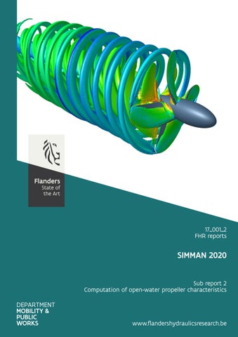
Cover figure
The Government of Flanders, Department of Mobility and Public Works, Flanders Hydraulics Research
Legal notice Flanders Hydraulics Research is of the opinion that the information and positions in this report are substantiated by the available data and knowledge at the time of writing. The positions taken in this report are those of Flanders Hydraulics Research and do not reflect necessarily the opinion of the Government of Flanders or any of its institutions. Flanders Hydraulics Research nor any person or company acting on behalf of Flanders Hydraulics Research is responsible for any loss or damage arising from the use of the information in this report. Copyright and citation The Government of Flanders, Department of Mobility and Public Works, Flanders Hydraulics Research, 2020 D/2020/3241/207 This publication should be cited as follows: sĂŶ ,ŽLJĚŽŶĐŬ͕ t͖͘ ůŽŽƚ͕ <͖͘ ĞůĞĨŽƌƚƌŝĞ͕ '͖͘ DŽƐƚĂĞƌƚ͕ &͘ (2020). SIMMAN 2020: Subreport 2 – Computation of open‐water propeller characteristics. Version 2.0. FHR Reports, 17_001_2. Flanders Hydraulics Research: Antwerp Reproduction of and reference to this publication is authorised provided the source is acknowledged correctly. Document identification Customer:
Flanders Hydraulics Research
Ref.:
WL2020R17_001_2
Keywords (3‐5):
Open‐Water, propeller, CFD
Knowledge domains:
Harbours and waterways Manoeuvring behaviour Open water Numerical calculations
Text (p.):
25
Confidentiality:
No
Author(s):
Van Hoydonck, W.
Appendices (p.):
22
Available online
Control Name Revisor(s):
Project leader:
Eloot, K.
Delefortrie, G.
Signature Getekend door:Katrien Eloot (Signature) Getekend op:2021-02-03 15:30:44 +01:0 Reden:Ik keur dit document goed
Getekend door:Guillaume Delefortrie (Sig Getekend op:2021-02-01 11:11:59 +01:0 Reden:Ik keur dit document goed
Approval Head of division:
F‐WL‐PP10‐5 version 24 VALID AS FROM: 25/11/2020
Mostaert, F.
Getekend door:Frank Mostaert (Signatur Getekend op:2021-02-01 12:59:39 +01:0 Reden:Ik keur dit document goed
SIMMAN 2020: Subreport 2 – Computation of open‐water propeller characteristics
Abstract The objective of this report is to investigate the possibility of determining open‐water propeller char‐ acteristics using Computational Fluid Dynamics (CFD). The propeller used in the current investigation is the four‐bladed propeller as used for the benchmark KRISO Very Large Crude Carrier 2 (KVLCC2) hull. The computed open‐water characteristics are not part of the CFD submission of Flanders Hy‐ draulics Research (FHR) for Workshop on Verification and Validation of Ship Manoeuvring Simulation Methods (SIMMAN). Computations are executed according to the specifications of the International Towing Tank Confer‐ ence (ITTC), where the angular velocity of the propeller remains constant and results are computed for a range of advance ratios 𝐽 by altering the forward velocity of the propeller. This contrasts with the recommendations of NUMECA for open‐water computations, where the forward velocity is held constant, and the advance ratio is changed by altering the angular velocity of the propeller. Compu‐ tations are executed in a rotating frame of reference which allows for larger time steps than in a fixed frame of reference. The by NUMECA recommended time step values were however not strict enough for low values of the advance ratio: the smallest value used is 1/8 of the recommended value. A com‐ parison between the numerical results and the reference values shows a good agreement. This type of computation could be used in the future as an alternative to experimentally determined open‐water propeller characteristics if a solution is found for the slow convergence at 𝐽 = 0.
Final version
WL2020R17_001_2
III
SIMMAN 2020: Subreport 2 – Computation of open‐water propeller characteristics
IV
WL2020R17_001_2
Final version
SIMMAN 2020: Subreport 2 – Computation of open‐water propeller characteristics
Contents Abstract........................................................................................................ III List of Figures ................................................................................................. VI List of Tables .................................................................................................. VII Nomenclature ................................................................................................ VIII 1 Introduction ............................................................................................... 1 2 Propeller geometry and computational setup ........................................................ 2.1 Propeller geometry .................................................................................. 2.2 Domain size and extents ............................................................................ 2.3 Grid generation ....................................................................................... 2.3.1 Initial mesh parameters ......................................................................... 2.3.2 Grid refinement .................................................................................. 2.3.3 Viscous layers ....................................................................................
4 4 6 7 7 7 8
3 Convergence analyses ................................................................................... 3.1 Grid convergence analysis........................................................................... 3.1.1 Derived grids ..................................................................................... 3.1.2 Simulation conditions ........................................................................... 3.1.3 Results ............................................................................................ 3.2 Time step convergence analysis ....................................................................
10 10 10 10 10 12
4 Determination of open‐water propeller characteristics ............................................. 4.1 Computational setup ................................................................................ 4.1.1 General............................................................................................ 4.1.2 Time step value and number of time steps ................................................... 4.1.3 Executing computations with negative inlet velocities ...................................... 4.1.4 Influence of Y+ on propeller blades............................................................ 4.2 Results ................................................................................................. 4.2.1 Convergence characteristics .................................................................... 4.2.2 Thrust and torque coefficients ................................................................. 4.2.3 Residual and force convergence characteristics .............................................. 4.2.4 Flow visualisations ............................................................................... 4.2.5 Computing times.................................................................................
14 14 14 14 15 15 16 16 16 18 20 20
5 Conclusions ............................................................................................... 24 References .................................................................................................... 25 A1 Numerical values for propeller characteristics ........................................................ A1 A2 Convergence of residuals, thrust and torque ......................................................... A2
Final version
WL2020R17_001_2
V
SIMMAN 2020: Subreport 2 – Computation of open‐water propeller characteristics
List of Figures Figure 1 Figure 2 Figure 3 Figure 4 Figure 5 Figure 6 Figure 7 Figure 8 Figure 9 Figure 10 Figure 11 Figure 12 Figure 13 Figure 14 Figure 15 Figure 16 Figure 17 Figure 18 Figure 19 Figure 20 Figure 21 Figure 22 Figure 23 Figure 24 Figure 25 Figure 26 Figure 27 Figure 28 Figure 29 Figure 30 Figure 31 Figure 32 Figure 33 Figure 34 Figure 35 Figure 36 Figure 37 Figure 38 Figure 39 Figure 40 Figure 41
VI
Open‐water characteristics of the KVLCC2 propeller at model scale. ...................... 2 IGES propeller geometry as provided on the SIMMAN website............................. 4 Geometry of model fairings (ITTC, 2014a). .................................................... 5 Construction of fairings and shaft. ............................................................. 5 Clip planes to separate one quarter of the hub geometry. .................................. 6 Geometry of the propeller with fairings and shaft............................................ 6 Side view of the computational domain. ...................................................... 7 Vertical cross section of the grid through the propeller axis. ............................... 8 Distribution of Y+ on the propeller blades. .................................................... 9 Propeller coefficient convergence as a function of grid size. ................................ 11 Propeller coefficient convergence as a function of grid size for a subset of three grids. . 11 Thrust 𝐾𝑇 and torque 𝐾𝑄 coefficient values as a function of time step. ................. 12 Computed and reference propeller characteristics versus advance ratio 𝐽 . .............. 16 Absolute and relative errors of the computed propeller characteristics versus 𝐽 . ....... 17 Polynomial fits (for 𝐽 ≥ 0.1) through the CFD results extrapolated to 𝐽 = 0. ........... 18 Convergence of the residuals for three advance ratios 𝐽 . ................................... 19 Convergence of the thrust and torque for three advance ratios 𝐽 . ........................ 19 Visualisation of the flow field around the propeller for three advance ratios 𝐽 . ......... 21 Normalised velocity profile in the propeller wake for three advance ratios. .............. 22 Location of velocity profiles in the wake of the propeller. ................................... 23 Convergence of the residuals, thrust and torque for 𝐽 = 0. ................................ A2 Convergence of the residuals, thrust and torque for 𝐽 = 0.05. ............................ A3 Convergence of the residuals, thrust and torque for 𝐽 = 0.1. .............................. A4 Convergence of the residuals, thrust and torque for 𝐽 = 0.15. ............................ A5 Convergence of the residuals, thrust and torque for 𝐽 = 0.20. ............................ A6 Convergence of the residuals, thrust and torque for 𝐽 = 0.25. ............................ A7 Convergence of the residuals, thrust and torque for 𝐽 = 0.3. .............................. A8 Convergence of the residuals, thrust and torque for 𝐽 = 0.35. ............................ A9 Convergence of the residuals, thrust and torque for 𝐽 = 0.40. ............................A10 Convergence of the residuals, thrust and torque for 𝐽 = 0.45. ............................A11 Convergence of the residuals, thrust and torque for 𝐽 = 0.5. ..............................A12 Convergence of the residuals, thrust and torque for 𝐽 = 0.55. ............................A13 Convergence of the residuals, thrust and torque for 𝐽 = 0.6. ..............................A14 Convergence of the residuals, thrust and torque for 𝐽 = 0.65. ............................A15 Convergence of the residuals, thrust and torque for 𝐽 = 0.70. ............................A16 Convergence of the residuals, thrust and torque for 𝐽 = 0.75. ............................A17 Convergence of the residuals, thrust and torque for 𝐽 = 0.8. ..............................A18 Convergence of the residuals, thrust and torque for 𝐽 = 0.85. ............................A19 Convergence of the residuals, thrust and torque for 𝐽 = 0.90. ............................A20 Convergence of the residuals, thrust and torque for 𝐽 = 0.95. ............................A21 Convergence of the residuals, thrust and torque for 𝐽 = 1.0. ..............................A22
WL2020R17_001_2
Final version
SIMMAN 2020: Subreport 2 – Computation of open‐water propeller characteristics
List of Tables Table 2 Table 3 Table 4 Table 5 Table 6 Table 7 Table 8 Table 9
Speed of advance 𝑉𝐴 as a function of the advance coefficient 𝐽 . ........................... Full‐scale and model scale propeller characteristics. .......................................... Grid cell sizes as a function of refinement level. ............................................... Characteristics of derived grids for the grid convergence analysis. .......................... Time step values as as function of the advance ratio 𝐽 . ...................................... Estimated values for the coefficients of the polynomials in Eqs. 8 and 9.................... Normalised computing times (minutes) as function of the advance ratio 𝐽 . ............... 𝐾𝑇 and 𝐾𝑄 values as a function of 𝐽 obtained in this research. ............................
Final version
WL2020R17_001_2
3 4 7 10 15 17 23 A1
VII
SIMMAN 2020: Subreport 2 – Computation of open‐water propeller characteristics
Nomenclature Abbreviations CFD DOF FHR ITTC KVLCC2 SIMMAN
VIII
Computational Fluid Dynamics Degree Of Freedom Flanders Hydraulics Research International Towing Tank Conference KRISO Very Large Crude Carrier 2 Workshop on Verification and Validation of Ship Manoeuvring Simulation Methods
WL2020R17_001_2
Final version
SIMMAN 2020: Subreport 2 – Computation of open‐water propeller characteristics
1 Introduction The mathematical models used in the simulators of FHR require input related to the forces and mo‐ ments acting on the hull for a range of parameters (such as drift angle, velocity, under‐keel clearance and draft), open‐water rudder and propeller characteristics and wind coefficients. FHR uses its tow‐ ing tank to determine the hull coefficients experimentally. The objective of this report is to determine open‐water propeller characteristics using CFD. The pro‐ peller used in the current investigation is the four‐bladed propeller as used in the SIMMAN for the benchmark KVLCC2 tanker1 . The resulting open‐water characteristics are not part of the CFD submis‐ sion of FHR for SIMMAN, but this type of data could be used in the future to remove the dependency on experimentally determined open‐water propeller characteristics as was the case now for the CFD computations submitted to SIMMAN (Van Hoydonck et al., 2020). The reference open‐water data is shown in Fig. 1. This graph shows the thrust and torque coefficients 𝐾𝑇 and 𝐾𝑄 and the efficiency 𝜂 as a function of the advance ratio 𝐽 . Apart from the reference data, the open‐water propeller characteristics for the KVLCC2 propeller as used at FHR are shown as well. The latter one is for a four‐bladed propeller with a diameter of 0.131 m. Note that the data as provided by SIMMAN are open‐water characteristics computed based on the propeller geometry, these were not obtained as part of open‐water tests carried out in an experimental facility. There is a significant difference of nearly 0.05 between the thrust coefficient 𝐾𝑇 for both model scale propellers for the full range of advance ratios. The differences for the torque coefficient 𝐾𝑄 are smaller, but still very visible. It is apparent that the propeller efficiency 𝜂 is not a good measure for judging the accuracy of computed propeller characteristics. As can be seen in Fig. 1, the difference between the two curves goes to zero for 𝐽 approaching zero despite the finite difference between the thrust coefficients near 𝐽 = 0. The thrust and torque coefficients 𝐾𝑇 and 𝐾𝑄 are defined using 𝑇 , 𝜌𝑛2 𝐷4 𝑄 𝐾𝑄 = , 𝜌𝑛2 𝐷5 𝐾𝑇 =
(1) (2)
where 𝜌 is the water density, 𝑛 = Ω/(2𝜋) the revolution rate (expressed in rotations per second) and 𝐷 the propeller diameter. The advance ratio 𝐽 is defined as 𝐽=
𝑉𝐴 , 𝑛𝐷
(3)
with 𝑉𝐴 the speed of advance of the propeller. The open‐water efficiency 𝜂 of the propeller is shown as well and is computed from 𝐾𝑇 and 𝐾𝑄 using 𝜂0 =
𝐾𝑇 𝐽 . 𝐾𝑄 2𝜋
(4)
The Reynolds number based on the blade chord length at 70 % of the blade radius is defined as 𝑅𝑒0.7 =
Final version
𝑐0.7 √𝑉𝐴2 + (0.7𝜋𝑛𝐷)2 , 𝜈 WL2020R17_001_2
(5)
1
SIMMAN 2020: Subreport 2 – Computation of open‐water propeller characteristics
Figure 1 – Open‐water characteristics of the KVLCC2 propeller at model scale as provided by SIMMAN and the data used at FHR.
in which 𝑐0.7 is the chord length at 0.7R and 𝜈 is the kinematic viscosity. According to ITTC (2014a), open‐water propeller tests should be executed with a constant revolution rate. The forward speed should be varied to produce results at different advance ratios. The highest value for 𝐽 should be selected such that 𝐾𝑇 < 0 in order to determine the zero‐crossing accurately. Here, a similar range will be used as the open water data provided by SIMMAN (0 < 𝐽 ≤ 1), with the same stepsize Δ𝐽 = 0.05. In the ITTC guidelines for CFD computations (ITTC, 2014b), it is mentioned that the variation of the ad‐ vance ratios 𝐽 can be achieved either by changing the angular velocity of the propeller or by changing the advance velocity. However, for very small values of 𝐽 , the angular velocity has to be increased by multiple orders of magnitude when the velocity is kept constant. This has a consequence for the grid generation process, because the Reynolds number would increase significantly. Therefore, the guidelines of ITTC (2014a) are followed in this investigation. For the current investigation, the rotation rate 𝑛 (1/s) of the open‐water data of the BSHC propeller is used (9.9 rps). This corresponds to an angular velocity of approximately 62.2 rad/s. The speed of advance of the propeller is computed using the advance ratio, fixed rotation rate and diameter, 𝑉𝐴 = 𝐽 𝑛𝐷.
(6)
For the current range of advance ratios, the resulting speed of advance is in the range 0 m/s to 2 m/s. The specific values of the speed of advance are required as input for the CFD computations and are listed in Table 2. In addition, the Reynolds numbers computed using Eq. 5 are shown as well.
1
2
See the website of SIMMAN: http://www.simman2019.kr/contents/KVLCC2.php.
WL2020R17_001_2
Final version
SIMMAN 2020: Subreport 2 – Computation of open‐water propeller characteristics Table 2 – Speed of advance 𝑉𝐴 as a function of the advance coefficient 𝐽.
𝐽
𝑉𝐴
𝑅𝑒0.7
𝐽
𝑉𝐴
𝑅𝑒0.7
0.0 0.05 0.1 0.15 0.2 0.25 0.3 0.35 0.4 0.45 0.5
0.0 0.100 98 0.201 96 0.302 94 0.403 92 0.5049 0.605 88 0.706 86 0.807 84 0.908 82 1.0098
1.755 × 10⁵ 1.756 × 10⁵ 1.757 × 10⁵ 1.759 × 10⁵ 1.763 × 10⁵ 1.767 × 10⁵ 1.772 × 10⁵ 1.777 × 10⁵ 1.784 × 10⁵ 1.792 × 10⁵ 1.800 × 10⁵
0.55 0.6 0.65 0.7 0.75 0.8 0.85 0.9 0.95 1.0
1.110 78 1.211 76 1.312 74 1.413 72 1.5147 1.615 68 1.716 66 1.817 64 1.918 62 2.0196
1.809 × 10⁵ 1.819 × 10⁵ 1.830 × 10⁵ 1.842 × 10⁵ 1.855 × 10⁵ 1.868 × 10⁵ 1.882 × 10⁵ 1.897 × 10⁵ 1.912 × 10⁵ 1.928 × 10⁵
Computation results will be compared against the reference data as provided by SIMMAN and both absolute (𝐸𝑎 (𝑆)) and relative errors (𝐸𝑟 (𝑆)) are computed: 𝐸𝑎 (𝑆) = 𝑆 − 𝐷, 𝐸𝑟 (𝑆) =
𝑆−𝐷 𝐸 (𝑆) × 100% = 𝑎 × 100%, 𝐷 𝐷
(7)
where 𝑆 is the computation result and 𝐷 is the reference value. The absolute and relative error are both shown because for very small reference values (near zero‐crossings), relative errors can become unbounded. This report is organised as follows. Chapter 2 discusses the propeller geometry and the compu‐ tational domain. Thereafter, a grid convergence study is executed to determine suitable meshing settings. In addition, in this chapter, a time step convergence analysis is executed as well, with the surprising result that FINE/Marine shows a time‐step instability. The computations use wall functions to model the boundary layer profile on the blades of the propeller. The influence on the results of removing this model from the CFD computations is investigated as well. Finally, results are computed for the same range of the advance ratio as shown in Fig. 1.
Final version
WL2020R17_001_2
3
SIMMAN 2020: Subreport 2 – Computation of open‐water propeller characteristics
2 Propeller geometry and computational setup 2.1
Propeller geometry
For the experiments of case 2.1 executed at BSHC, the model ship has a scale factor of 1/45.714. The four‐bladed propeller that was used in these experiments deviates from the full‐scale propeller. The full‐scale and model scale propeller characteristics (including the characteristics of the KVLCC2 propeller used at FHR) are shown in Table 3. The IGES model as provided by SIMMAN is shown in Fig. 2. Table 3 – Full‐scale and model scale propeller characteristics.
Parameter
Prototype
BSHC model
FHR model
No. of blades D/m P/D (0.7R) Ae/A0 Hub ratio
4 9.86 0.721 0.431 0.155
4 0.204 0.808 0.448 0.165
4 0.131 0.793 0.52 0.192
Figure 2 – IGES propeller geometry as provided on the SIMMAN website.
4
WL2020R17_001_2
Final version
SIMMAN 2020: Subreport 2 – Computation of open‐water propeller characteristics
The ITTC procedure concerning Open Water Tests (ITTC, 2014a) mentions that the fairings forward and aft of a conventional pushing propeller should be modelled according to Fig. 3. Hence, the pro‐ peller geometry as provided by SIMMAN had to be adapted in Rhino. Due to the larger diameter at the front of the propeller hub than at the back, the length of the fairing (63 mm) was set to three times the radius of the boss at the forward end (21 mm), see Fig. 4. This length is equal to the minimum value as suggested in Fig. 3. The fairing is constructed with an elliptic curve with matching tangent at the hub. At the aft part of the hub, a straight conical section is added with matching tangent that intersects a shaft with a diameter of 20 mm.
Figure 3 – Geometry of model fairings (ITTC, 2014a).
21.00
14.45
10.00
24.61
50.00
63.00
Figure 4 – Construction of fairings and shaft.
The original CAD model contains only one blade and half of the hub geometry. One quarter section of the hub is separated using two cut planes that are rotated 90° along the X‐axis (see Fig. 5). The resulting hub section together with the blade and fillets is replicated three times around the X‐axis, Final version
WL2020R17_001_2
5
SIMMAN 2020: Subreport 2 – Computation of open‐water propeller characteristics
the fairing and shaft are revolved 360° around the X‐axis, giving the complete geometry as shown in Fig. 6. The length of the shaft is 2000 mm. The original IGES file, the modified geometry (Rhino 3dm file) and a cleaned Parasolid model ready for use in FINE/Marine have been added to the CFD CAD model repository of FHR2 .
Figure 5 – Clip planes to separate one quarter of the hub geometry.
Figure 6 – Geometry of the propeller with fairings and shaft.
2.2
Domain size and extents
The computational domain is a cylinder with the propeller located at its centreline. The dimensions of the cylinder are approximately an integer multiple of the propeller radius: the length 𝐿𝑑 equals 24 R and the diameter 𝐷𝑑 is 20 D. In absolute values, the length and diameter equate to 𝐿𝑑 = 2.43 m and 𝐷𝑑 = 2.03 m. The propeller is located at 𝐿𝑑 /3 from the inlet. An overview of the domain is shown in Fig. 7. 2
6
See here: https://wlwiki.vlaanderen.be/display/wlwiki/T0Z_prop
WL2020R17_001_2
Final version
SIMMAN 2020: Subreport 2 – Computation of open‐water propeller characteristics
2.03 m
2.43 m
Figure 7 – Side view of the computational domain.
2.3 2.3.1
Grid generation Initial mesh parameters
The initial Cartesian mesh consists of 76 800 cells: 48 cells in the X‐direction and 40 cells in both the Y‐ and Z‐direction. In absolute values, these cubic cells have a rib length of approximately 0.05 m.
2.3.2
Grid refinement
The global maximum number of refinements was set to 12. Table 4 shows the absolute sizes of cells for all refinement levels. The cell sizes relative to the propeller radius are approximately 10 times as large. Table 4 – Grid cell sizes as a function of refinement level.
refinement level
absolute cell size/m
refinement level
absolute cell size/m
0 1 2 3 4 5 6
5.064 × 10⁻² 2.532 × 10⁻² 1.266 × 10⁻² 6.330 × 10⁻³ 3.165 × 10⁻³ 1.583 × 10⁻³ 7.913 × 10⁻⁴
7 8 9 10 11 12
3.956 × 10⁻⁴ 1.978 × 10⁻⁴ 9.891 × 10⁻⁵ 4.946 × 10⁻⁵ 2.473 × 10⁻⁵ 1.236 × 10⁻⁵
All domain boundary faces are active for refinement except for the three faces that make up the outer domain. Faces are logically combined in seven groups, with five groups related to the propeller Final version
WL2020R17_001_2
7
SIMMAN 2020: Subreport 2 – Computation of open‐water propeller characteristics
blades and two groups related to the shaft and the hub with the cap. The fillets, leading edges and trailing edges are refined eight times, the blade tips are refined nine times. The pressure and suction sides of the blade surfaces are refined six times. The cap and hub are refined five times. The shaft and the conic taper located aft of the propeller are also refined five times with the difference that nonzero values are set for the target cell sizes: 0.0038 m, 0.0019 m and 0.0019 m. This results in cells near the shaft that are stretched in the X‐direction. This is visible in Fig. 8, which shows a vertical cross section of the grid through the propeller axis. The blade edges are activated for refinement as well: they are refined eight times. In order to capture the vortical wake of the propeller, a refinement sector is defined that envelopes the propeller and the frontal half of the shaft. Absolute target cell sizes are set to 1/10 of the initial cell size (which corresponds to four refinements). For cases where the propeller operates in reverse flow conditions (third quadrant), the grid refinement for the wake should be extended upstream. This is not persued here and left as a recommendation for future work.
Figure 8 – Vertical cross section of the grid through the propeller axis.
2.3.3
Viscous layers
For the initial grid, the viscous boundary layers are approximated with wall functions. Later on, the effect of resolving the boundary layer will be checked as well. The reference length and velocity were set to 0.1 m and 4.5 m/s respectively. With a target Y+ of 100, the height of the first cell in the boundary layer is 6.9 × 10⁻³ m. With the size of the grid generated for the Euler mesh, the required number of layers varies from one to three. The minimum number of layers was kept at its default (two), which means that actual Y+ values will very likely be lower than 100, especially on faces where two layers are inserted where only one layer is strictly required. This is confirmed in Fig. 9, which shows the Y+ values on the pressure and suction sides of the propeller blades. The maximum value is close to 100, while the minimum value is smaller than 1. The average equals 47. After inserting viscous layers, the grid size for the base mesh equals 6.97 × 10⁶ cells. Concerning the grid quality, the minimum orthogonality equals 14.75° which is higher than the recommended minimum of 10°.
8
WL2020R17_001_2
Final version
SIMMAN 2020: Subreport 2 – Computation of open‐water propeller characteristics
Figure 9 – Distribution of Y+ on the propeller blades.
Final version
WL2020R17_001_2
9
SIMMAN 2020: Subreport 2 – Computation of open‐water propeller characteristics
3 Convergence analyses 3.1 3.1.1
Grid convergence analysis Derived grids
A grid convergence analysis is executed to verify that computed integral values of thrust and torque converge to a grid‐independent value. It is limited to a comparison of the computed values as a function of the grid size, without looking at the convergence characteristics in detail. Five derived grids have been constructed from the base grid that was discussed in the previous chapter. Due to the size of the base grid, only coarser grids have been constructed. Table 5 lists the factors used to coarsen the initial Cartesian mesh of the base mesh together with the final cell count of the meshes. Table 5 – Characteristics of derived grids for the grid convergence analysis.
3.1.2
grid
refinement factor
grid size 𝑛𝑖
3 √𝑛 1 /𝑛𝑖
base coarse 1 coarse 2 coarse 3 coarse 4 coarse 5
1 0.9 0.8 0.7 0.64 0.49
6.97 × 10⁶ 5.86 × 10⁶ 4.86 × 10⁶ 4.00 × 10⁶ 3.58 × 10⁶ 2.45 × 10⁶
1 1.06 1.13 1.2 1.25 1.42
Simulation conditions
The computations were set up such that the propeller location is fixed in space and a non‐zero inflow is defined at the upward boundary of the domain and its cylindrical side. At the outflow, the pressure is prescribed. The x‐velocity at the inlet is set to −1.18 m/s, which corresponds to an advance ratio of 𝐽 = 0.58. These settings are different from the settings used in the final computations, where the relative fluid velocity is set by defining a body motion for the propeller in still water as prescribed by the ITTC (2014a).
3.1.3
Results
The thrust and torque are shown as a function of the grid size. By using more than three grids, smooth approximations could be fitted through the data to reduce the influence of outliers in the results. On the other hand, one could use a subset of the data to show convergence. The thrust coefficient, torque coefficient and efficiency of the propeller are shown in Fig. 10 as a function of the relative grid size of the computations.3 Results converge if globally speaking, the 3
Note that for the computation of the propeller characteristics (thrust and torque coefficients and its efficiency), only the contri‐ butions of the individual blades are included.
10
WL2020R17_001_2
Final version
SIMMAN 2020: Subreport 2 – Computation of open‐water propeller characteristics
curve flattens out to the left. Although in value close to the results for the finest grid, it is clear that the right‐most data points (coarsest grid) do not follow the trend of the finer grids. The results for grids coarse 1 and coarse 3 diverges somewhat from the converging trend that is visible with base, coarse 2 and coarse 4 with respective refinement factors of 1, 0.8 and 0.64. These last three are shown in Fig. 11. This last figure shows monotonic convergence for 𝐾𝑇 , 10𝐾𝑄 and 𝜂. Based on these results, the final computations to determine the open‐water characteristics of this propeller, are executed using the middle grid with 4.86 × 10⁶ cells.
Figure 10 – Propeller coefficient convergence as a function of grid size.
Figure 11 – Propeller coefficient convergence as a function of grid size for a subset of three grids: base, coarse 2 and coarse 4.
Final version
WL2020R17_001_2
11
SIMMAN 2020: Subreport 2 – Computation of open‐water propeller characteristics
3.2
Time step convergence analysis
Apart from the grid convergence analyses presented in the previous section, a time step convergence analysis was executed because it appears that the NUMECA recommended practice for the time step value for this type of computation is not sufficient. NUMECA advises to use 20 time steps per revolu‐ tion when the rotation frame approach is used. For the current setup, the rotation rate is 9.9 rps, which corresponds to a time step of Δ𝑡 = 0.005 s. This value is sufficient to get converging results for 𝐽 > 0.5, but for lower values of 𝐽 , the solution does not converge. Initially, it was thought to be caused by the grid, but tests revealed that with smaller time steps, results do converge. Part of the discrepancy between results obtained at FHR and the recommended practice of NUMECA might be caused by the fact that the latter does not follow the guidelines of the ITTC (2014a): NUMECA opts to obtain the open‐water performance curve by varying the angular velocity of the propeller combined with a constant inlet velocity whereas ITTC dictates that the angular velocity should remain constant for the complete range of advance ratios. Here, a time step convergence analysis is executed with a fine grid that does not use wall functions on the propeller blades and an expansion ratio inside the viscous layers of 1.15, which is lower than the default value of HEXPRESS of 1.2. The grid contains 13.562 × 10⁶ cells. Computations are executed at one value of the advance ratio: 𝐽 = 0.5. Values for the thrust and torque coefficients as a function of the time step are presented in Fig. 12. This graph shows clearly that as the time step is decreased, the difference between the values increases. Although the actual differences in the values are very small (fifth significant digit), this result prevents a conclusion on the minimum required time step for this type of computation. A support request (#29341) was opened to notify the software developers of this issue.
Figure 12 – Thrust 𝐾𝑇 and torque 𝐾𝑄 coefficient values as a function of time step.
While executing computations for the complete range of advance ratios, it was found that with low values of 𝐽 , it takes longer for the solver to find a converged solution. Support was also notified 12
WL2020R17_001_2
Final version
SIMMAN 2020: Subreport 2 – Computation of open‐water propeller characteristics
of this issue, with the response being to increase the domain. At zero forward speed the propeller acts to pump the fluid around the domain: the boundary conditions at the domain boundaries (in‐ let, outlet and side) are set to zero velocity. This means there is no implicit flow direction that can help stabilise the solution. This can take a very large amount of time to settle, and one may even experience convergence issues if the time step is chosen too large. For this condition, an alterna‐ tive was tested where the boundary condition type for the domain sides was changed to solid walls with wall functions. This seems to converge better than the original outflow boundary condition that prescribes the pressure4 .
4 However, changing the boundary condition type for a domain did not seem to be a good idea: afterwards, the original boundary condition types were restored to execute an additional computation at a high advance ratio, but this computation would not converge (even with a lot of persuasion from the author’s part). A solution was found by duplicating the project, copying the mesh, setting the correct boundary conditions and executing the extra computation in that new project folder.
Final version
WL2020R17_001_2
13
SIMMAN 2020: Subreport 2 – Computation of open‐water propeller characteristics
4 Determination of open‐water propeller char‐ acteristics In this chapter, the setup of the final computations to determine the open‐water propeller charac‐ teristics is discussed. Issues with the setup and/or the execution of the computations are discussed. The results are shown and they are put in perspective.
4.1 4.1.1
Computational setup General
The computational setup for the final set of computations is slightly different from the setup used for the grid convergence analysis discussed in section 3.1. The linear motion of the propeller with respect to the surrounding fluid is now set by applying a linear motion to the propeller instead of to the fluid, as per the requirements of ITTC. Hence, the surge Degree Of Freedom (DOF) (Tx0) is imposed with a 1/2 sinusoidal ramp with an initial time 𝑡0 of 0 s, a final time 𝑡1 of 0.5 s, an initial velocity 𝑉0 of 0 m/s and a final velocity 𝑉1 corresponding to an advance ratio between 0 and 1 as shown in Table 2. The final angular velocity of the propeller is fixed at 62.2 rad/s, with a 1/2 sinusoidal ramp with the same time parameters as defined for the surge motion definition. As a consequence of setting the forward velocity of the propeller, all components of the patches (inlet and cylinder side) where the Far field boundary condition is defined, are set to zero. In the Mesh Management menu, the Rotating frame method is activated and the mesh displacement definition follows the rigid motion of the propeller body. The initial solution for the computations is always started from a uniform still velocity field. Initially, the strategy was to start from a previous computation with a similar (slightly higher or lower) advance ratio to speed up convergence but this seemed to give issues with the propeller velocities that were not (always) set to the correct value. The rest of the setup is fairly standard: the computations are setup as unsteady with a single fluid (standard fresh water at 15 °C: 𝜌 = 999.1026 kg/m3 and 𝜇 = 0.001 138 Pa ⋅ s). The turbulence model used is the Explicit Algebraic Stress Model (EASM). The reference parameters are 𝐿𝑟𝑒𝑓 = 0.101 286 m and 𝑉𝑟𝑒𝑓 = 4.838 m/s. With these values, the Reynolds number equals 4.3021 × 10⁵ . Regarding the boundary conditions for the the solid surfaces, all patches that belong to the propeller blades are configured to use wall functions. The solid patches belonging to the shaft are configured as slip surfaces.
4.1.2
Time step value and number of time steps
As mentioned before, the time step value and the number of time steps had to be modified for the small advance ratios to ensure that the computations converged properly. 14
WL2020R17_001_2
Final version
SIMMAN 2020: Subreport 2 – Computation of open‐water propeller characteristics
Table 6 contains the time step values that were used for the final computations. For values of 𝐽 > 0.4, a value of Δ𝑡 = 0.002 s is used. For advance ratios between 𝐽 = 0.2 and 𝐽 = 0.4, the time step was halved to Δ𝑡 = 0.001 s get sufficiently converging results. For lower advance ratios, Δ𝑡 = 0.0005 s. The total number of time steps varied between 5000 for advance ratios above 𝐽 = 0.4, to at least 25 000 time steps for 𝐽 = 0.05. Table 6 – Time step values as as function of the advance ratio 𝐽 to get sufficiently converging results.
4.1.3
𝐽
Δ𝑡/𝑠
𝐽
Δ𝑡/𝑠
0.0 0.05 0.1 0.15 0.2 0.25 0.3 0.35 0.4 0.45 0.5
0.0005 0.0005 0.0005 0.0005 0.001 0.001 0.001 0.001 0.002 0.002 0.002
0.55 0.6 0.65 0.7 0.75 0.8 0.85 0.9 0.95 1.0
0.002 0.002 0.002 0.002 0.002 0.002 0.002 0.002 0.002 0.002
Executing computations with negative inlet velocities
When the propeller velocity is negated (and otherwise nothing is changed), the fluid flow relative to the propeller is towards the inlet, while the wake is still pushed aft by the propeller. If this con‐ dition works well, it might be possible to get a better prediction of the resulting values near J=0 by interpolating instead of by extrapolating the data. For a single computation, the boundary conditions on the inlet and outlet were switched and the longitudinal velocity of the propeller was set to 𝑉𝑝𝑟𝑜𝑝 = −0.403 92 m/s. With these conditions, a timestep of Δ𝑡 = 0.001 s and a total of 20 000 iterations, the computation does not converge very well (especially not when compared to computations with a high positive advance ratio), although the solution looks reasonable. In a reverse flow condition, the wake will not move backward as far as with positive advance ratios. It will expand and move downstream towards the propeller again. This may cause difficulties with convergence, as part of the wake may be ingested by the propeller again. In helicopter literature, this flow condition is called vortex ring state. With even higher negative velocities of the propeller, the wake will be swept directly upstream, with the propeller operating as a wind turbine extracting energy from the surrounding fluid. The wake will expand and the velocity inside the wake will be lower than the surrounding fluid velocity.
4.1.4
Influence of Y+ on propeller blades
Some computations were executed with viscous layers fine enough to resolve the boundary layer around the propeller blades without the need for wall functions. The differences with the results obtained with coarser meshes that do use wall functions to model the boundary layer profile were small enough to justify the use of wall functions. Final version
WL2020R17_001_2
15
SIMMAN 2020: Subreport 2 – Computation of open‐water propeller characteristics
4.2 4.2.1
Results Convergence characteristics
The convergence characteristics of the field variables (pressure, velocity components and turbulent quantities) can be used to judge the convergence of a computation.
4.2.2
Thrust and torque coefficients
The absolute values of 𝐾𝑇 , 𝐾𝑄 and 𝜂 computed with FINE/Marine are shown in Fig. 13 together with the reference data as provided by SIMMAN. The absolute and relative errors of these quantities are shown in Fig. 14. Due to the definition of the propeller efficiency 𝜂, the relative error of this quantity for 𝐽 = 0 cannot be computed (division by zero). For the majority of advance values, the relative error 𝐸𝑟 for 𝐾𝑇 is less than five percent. Only near the extremities of 𝐽 does 𝐸𝑟 increase beyond this value. Due to the difference in the location of the zero crossing between the reference data and the computed values, the relative errors for 𝐾𝑇 and 𝜂 becomes very large for 𝐽 ≥ 0.85. Except for the extreme values of 𝐽 , the relative error for 𝐾𝑄 is less than 5%. Investigating the predicted trendlines, it is clear that the results for 𝐽 = 0 diverge and do not respond to the common parabolic trend. This is likely caused by the different far‐field boundary conditions used for this case. Whereas for the cases with 𝐽 > 0, external boundary conditions are used because of the motion of the propeller relative to the surrounding fluid, for 𝐽 = 0 this proved too unstable and the boundary conditions for the domain boundaries were altered to solid walls.
Figure 13 – Computed and reference propeller characteristics (𝐾𝑇 , 𝐾𝑄 and 𝜂) versus advance ratio 𝐽.
To improve the prediction of the result at 𝐽 = 0, a polynomial curve is fit through the data for 𝐽 ≤ 0.1. The polynomial is then evaluated at 𝐽 < 0.1 to obtain alternative coefficient values that 16
WL2020R17_001_2
Final version
SIMMAN 2020: Subreport 2 – Computation of open‐water propeller characteristics
Figure 14 – Absolute (top) and relative (bottom) errors of the computed thrust coefficient (𝐾𝑇 ), torque coefficient (𝐾𝑄 ) and efficiency (𝜂) versus advance ratio 𝐽.
follow a smooth trend over the complete advance ratio range. The reference data is used to deter‐ mine the degree and coefficients of the polynomial curve and to verify that the predicted values of 𝐾𝑇 and 𝐾𝑄 for 𝐽 < 0.1 are close to the reference values. Least‐squares estimates of both quad‐ ratic, cubic and quartic polynomials were constructed using LMFIT5 . The coefficient estimates using the quartic polynomials gave the smallest errors at 𝐽 = 0, hence fourth‐degree curve fits were con‐ structed: 𝐾𝑇 (𝐽 ) = 𝑎𝐽 4 + 𝑏𝐽 3 + 𝑐𝐽 2 + 𝑑𝐽 + 𝑒; 𝐾𝑄 (𝐽 ) = 𝑎𝐽 4 + 𝑏𝐽 3 + 𝑐𝐽 2 + 𝑑𝐽 + 𝑒.
(8) (9)
The coefficient values for both polynomials are shown in Table 7. Table 7 – Estimated values for the coefficients of the polynomials in Eqs. 8 and 9.
a b c d e
𝐾𝑇
𝐾𝑄
−0.2100 ± 0.0158 0.4160 ± 0.0350 −0.3920 ± 0.0264 −0.208 00 ± 0.007 81 0.337 000 ± 0.000 731
−0.1120 ± 0.0193 0.0350 ± 0.0427 −0.1220 ± 0.0323 −0.218 00 ± 0.009 54 0.395 000 ± 0.000 893
The extrapolated fits are shown in Fig. 15 together with the values obtained from CFD and the ref‐ erence values. It is apparent that for both 𝐾𝑇 and 𝐾𝑄 the numerical value for 𝐽 = 0.05 is slightly lower than the polynomial fit through the data, while the numerical values at 𝐽 = 0 are higher than 5
Non‐Linear Least‐Squares Minimization and Curve‐Fitting for Python: https://lmfit.github.io/lmfit-py/index.html.
Final version
WL2020R17_001_2
17
SIMMAN 2020: Subreport 2 – Computation of open‐water propeller characteristics
the polynomials. The numerical values of the coefficients as obtained in this research are displayed in Table 9 in Appendix A1.
Figure 15 – Polynomial fits (for 𝐽 ≥ 0.1) through the CFD results extrapolated to 𝐽 = 0.
4.2.3
Residual and force convergence characteristics
The convergence of the residuals for 𝐽 = 0.2, 0.5 and 0.8 are shown in Fig. 16. The advance ratio has a significant effect on the speed of convergence: with higher linear velocities of the propeller, residuals drop quicker to an acceptable level. For the results at 𝐽 = 0.2, the graph shows that convergence of the residuals of momentum (𝑈 , 𝑉 and 𝑊 ) is poor. The trend does not level off to a final value similar to the curves for the two higher values of 𝐽 . The level of convergence of the pressure 𝑃 and turbulent kinetic energy 𝐾 residuals is almost not influenced by the advance ratio, although for the latter, the speed of convergence is affected significantly: it takes significantly longer for the lowest value of 𝐽 . Convergence of the specific dissipation 𝜔 is affected significantly by 𝐽 . For the lowest advance ratio shown in Fig. 16, the residual value levels off at 10 × 10−1 and increases slightly as time progresses. Fig. 17 shows the convergence of the computed thrust and torque on the propeller blades. After one second (1/10th of the total computation time), the values of 𝑇 and 𝑄 have converged to an acceptable level, also for 𝐽 = 0.2.
18
WL2020R17_001_2
Final version
SIMMAN 2020: Subreport 2 – Computation of open‐water propeller characteristics
Figure 16 – Convergence of the residuals of velocity (𝑈, 𝑉 and 𝑊 ), pressure (𝑃 ), turbulent kinetic energy (𝐾) and specific dissipation 𝜔 for three advance ratios 𝐽.
Figure 17 – Convergence of the thrust and torque for three advance ratios 𝐽.
Final version
WL2020R17_001_2
19
SIMMAN 2020: Subreport 2 – Computation of open‐water propeller characteristics
4.2.4
Flow visualisations
For the three advance ratios discussed in § 4.2.3, visualisations of the flow are shown in Fig. 18. In a vertical plane, the magnitude of the relative linear velocity is shown. On the propeller geometry, the pressure is displayed. The vortical structures generated by the lifting surfaces are visualised using 𝑄 an isosurface of the Q‐criterion normalised with ‖∇(𝑈 )‖, (𝑄′ = ‖∇(𝑈)‖ = 2) coloured with heli‐ city. Due to the fairly coarse resolution in the wake, the tip vortices are visible for a relatively short dis‐ tance behind the propeller plane. The longitudinal spacing between the tip vortices of the propeller blades increases with increasing 𝐽 . For the low advance ratios, the inner vortex sheet (which has the opposite helicity as compared to the tip vortex) quickly rolls up in concentrated vortex that extends far downstream. At three positions (𝑥 = 𝑅, 2𝑅, 4𝑅) in the wake of the propeller, the velocity profile has been ex‐ tracted (Fig. 19). The locations are shown in Fig. 20. The velocity profile is normalised by the inflow 𝑉𝐴 , and the radial distance is normalised by the propeller radius 𝑅. Note that the velocity profiles are not azimuthally averaged, but taken at a fixed azimuth behind the propeller. As a consequence, the velocity profile close to the propeller may be affected by the presence of concentrated vorticity released at the blade tips. The average relative velocity (computed between the shaft and 𝑟/𝑅 = 1) for each position is shown with a vertical line. As expected, lower advance ratios result in higher relative velocities in the wake. For all cases, the highest average velocity in the wake is attained at 𝑥 = 4𝑅, except for 𝐽 = 0.2, where the highest average velocity is found at 𝑥 = 2𝑅. Due to the slip boundary condition set for the propeller shaft, the velocity at the shaft does not reduce to zero at the smallest radial distance. For the two lowest advance ratios shown, the maximum value in the velocity profile is more spread out than at the highest advance ratio. For 𝐽 = 0.2, the velocity field diffuses outward more rapidly than with the higher advance ratios.
4.2.5
Computing times
For the setup of the computations as described in this report, computing times are shown in Table 8. All computations were executed on the navier queue with FINE/Marine 8.2, mostly using 96 pro‐ cessors. For computations that were run using a different number of processors, the computing times have been adapted proportionally. For computations executed at some of the lower advance ratios, the displayed computing times are the sum of two separate computations (due to restarting it with a different/smaller time step value). Increasing the advance ratio has an overall positive effect on the computing times. Note that the computations were run for a fixed number of time steps. In the newest version of FINE/Marine, convergence of a computation can be checked with a conver‐ gence checker that will stop the execution once a predefined convergence level has been attained. For a four‐bladed propeller as used in this study, using the periodicity boundary condition that has been added recently to FINE/Marine, one could reduce the domain geometry to one quarter of the propeller geometry6 . In theory, this should reduce the computing times as shown in Table 8 with a factor four.
6
At the time the computations were configured, the periodicity boundary condition in FINE/Marine 8.2 only worked for computa‐ tions with periodicity defined around the Z‐axis and grids should be constructed using Autogrid instead of HEXPRESS.
20
WL2020R17_001_2
Final version
SIMMAN 2020: Subreport 2 – Computation of open‐water propeller characteristics
(a)
𝐽 = 0.2.
(b)
𝐽 = 0.5.
(c)
𝐽 = 0.8.
Figure 18 – Visualisation of the flow field around the propeller for three advance ratios 𝐽. Magnitude of relative velocity in the 𝑦 = 0 plane, the vortical wake coloured with helicity and surface pressure on the propeller geometry.
Final version
WL2020R17_001_2
21
SIMMAN 2020: Subreport 2 – Computation of open‐water propeller characteristics
Figure 19 – Normalised velocity profile and average value in the wake of the propeller at three locations aft of the propeller plane (𝑥 = 𝑅, 2𝑅, 4𝑅) for three advance ratios 𝐽.
22
WL2020R17_001_2
Final version
SIMMAN 2020: Subreport 2 – Computation of open‐water propeller characteristics
Figure 20 – Location of velocity profiles in the wake of the propeller.
Table 8 – Normalised computing times (minutes) as function of the advance ratio 𝐽.
Final version
𝐽
𝑡𝑐
𝐽
𝑡𝑐
0.0 0.05 0.1 0.15 0.2 0.25 0.3 0.35 0.4 0.45 0.5
2000 990 1500 1550 1104 916 774 908 504 540 348
0.55 0.6 0.65 0.7 0.75 0.8 0.85 0.9 0.95 1.0
367 342 376 343 359 343 338 345 361 338
WL2020R17_001_2
23
SIMMAN 2020: Subreport 2 – Computation of open‐water propeller characteristics
5 Conclusions As part of the SIMMAN project (17_001) at FHR, research was conducted to investigate the feasibil‐ ity of computing open‐water propeller characteristics using the commercial CFD software package FINE/Marine. The KVLCC2 propeller and reference open‐water data as provided on the SIMMAN website is used. The test conditions for the shallow water computations were executed with a 1/45.714 scale model at BSHC. The model‐scale propeller has a diameter of 0.204 m. No experi‐ ments were executed with this propeller to determine its open‐water characteristics, instead, the open‐water data was computed. This fact was only discovered when the computational results were compared with the reference data. A comparison of the open‐water propeller data of FHR for the KVLCC2 propeller with the data as provided by SIMMAN shows that significant differences are present between the two data sets. There are three probable causes: both propellers do not have exactly the same geometry, the scale of the propellers is different and the method to obtain the data for both propellers is not the same. The computational setup in FINE/Marine mimics the requirements of ITTC for the setup of open‐ water tests, where the advance ratio is altered by changing the forward velocity of the propeller while its angular velocity is kept constant. This contrasts with the recommended practice of NUMECA where the propeller angular velocity is modified to change the advance ratio. The FINE/Marine setup uses a rotating frame method to reduce the computation time. Two convergence studies have been executed: one where the dependency of the grid density on the convergence of the results is inves‐ tigated, and a second one where the influence of the time step on the convergence characteristics is investigated. The latter one shows the surprising result that as the time step is reduced, results show a diverging trend. This convergence analysis was executed because it was found that with lower advance ratios, results converged only very slowly, or not at all with the recommended time step settings. Lowering the time step value improved convergence, but it still proved difficult with very low advance ratios. With the propeller operating in still water (𝐽 = 0), the boundary conditions had to be changed. All boundary condition types of the faces of the cylindrical domain were changed to solid boundaries. This change in combination with a reduced time step improved convergence characteristics over using the standard (external) boundary conditions. A comparison of the computed results with the reference data shows that the resulting 𝐾𝑇 and 𝐾𝑄 curves are very similar, for the majority of advance ratio values, relative errors are less than 5 %. Relative errors do become larger near the zero‐crossing of the curves (𝐽 ≈ 1) due to the diminishing value of the reference. Due to the definition of the propeller efficiency 𝜂, comparing the computed efficiency with the efficiency of the reference data is not useful. By fitting a polynomial through the computational results for 𝐽 ≤ 0.1, it is possible to find estimates for 𝐾𝑄 and 𝐾𝑇 for 𝐽 < 0.1 that follow a smooth curve over the complete advance ratio range. The exact origin of the reference data as provided by SIMMAN is unknown. With the knowledge gained in this research, it is recommended to compute using CFD open‐water propeller characteristics for a propeller for which FHR has experimental open‐water data available.
24
WL2020R17_001_2
Final version
SIMMAN 2020: Subreport 2 – Computation of open‐water propeller characteristics
References ITTC (2014a). ITTC – Recommended Procedures and Guidelines ‐ Open water test. 7.5‐02‐03‐02.1 (Revision 03). ITTC. p. 10 ITTC (2014b). ITTC – Recommended Procedures and Guidelines ‐ Practical guidelines for RANS calculation of nominal wakes. 7.5‐03‐03‐02 (Revision 00). ITTC. p. 9 Van Hoydonck, W.; Delefortrie, G.; Eloot, K. (2020). ‘Prediction of Hydrodynamic Forces on KVLCC2 in Shallow Water using RANS Simulations’. Submitted to SIMMAN 2020: Workshop on Verification and Validation of Ship Manoeuvring Simulation Methods
Final version
WL2020R17_001_2
25
SIMMAN 2020: Subreport 2 – Computation of open‐water propeller characteristics
A1 Numerical values for propeller characterist‐ ics Table 9 – 𝐾𝑇 and 𝐾𝑄 values as a function of 𝐽 obtained in this research.
Final version
𝐽
𝐾𝑇 (𝐶𝐹 𝐷)
10𝐾𝑄 (𝐶𝐹 𝐷)
𝐾𝑇 (𝑓𝑖𝑡)
10𝐾𝑄 (𝑓𝑖𝑡)
0.00 0.05 0.10 0.15 0.20 0.25 0.30 0.35 0.40 0.45 0.50 0.55 0.60 0.65 0.70 0.75 0.80 0.85 0.90 0.95 1.00
0.3447 0.3224 0.3125 0.2989 0.2832 0.2664 0.2488 0.2309 0.2124 0.1936 0.1743 0.1546 0.1343 0.1134 0.0919 0.0698 0.0469 0.0236 ‐0.0015 ‐0.0279 ‐0.0563
0.4055 0.3811 0.3715 0.3601 0.3470 0.3330 0.3184 0.3033 0.2875 0.2709 0.2532 0.2342 0.2138 0.1918 0.1679 0.1423 0.1146 0.0851 0.0524 0.0170 ‐0.0216
0.3371 0.3258 0.3128 0.2985 0.2829 0.2664 0.2491 0.2311 0.2126 0.1936 0.1742 0.1543 0.1341 0.1133 0.0920 0.0700 0.0472 0.0234 ‐0.0016 ‐0.0280 ‐0.0562
0.3949 0.3837 0.3720 0.3596 0.3466 0.3330 0.3187 0.3036 0.2877 0.2709 0.2530 0.2339 0.2135 0.1916 0.1680 0.1425 0.1149 0.0849 0.0524 0.0170 ‐0.0216
WL2020R17_001_2
A1
SIMMAN 2020: Subreport 2 – Computation of open‐water propeller characteristics
A2 Convergence of residuals, thrust and torque
Figure 21 – Convergence of the residuals, thrust and torque for 𝐽 = 0.
A2
WL2020R17_001_2
Final version
SIMMAN 2020: Subreport 2 – Computation of open‐water propeller characteristics
Figure 22 – Convergence of the residuals, thrust and torque for 𝐽 = 0.05.
Final version
WL2020R17_001_2
A3
SIMMAN 2020: Subreport 2 – Computation of open‐water propeller characteristics
Figure 23 – Convergence of the residuals, thrust and torque for 𝐽 = 0.1.
A4
WL2020R17_001_2
Final version
SIMMAN 2020: Subreport 2 – Computation of open‐water propeller characteristics
Figure 24 – Convergence of the residuals, thrust and torque for 𝐽 = 0.15.
Final version
WL2020R17_001_2
A5
SIMMAN 2020: Subreport 2 – Computation of open‐water propeller characteristics
Figure 25 – Convergence of the residuals, thrust and torque for 𝐽 = 0.20.
A6
WL2020R17_001_2
Final version
SIMMAN 2020: Subreport 2 – Computation of open‐water propeller characteristics
Figure 26 – Convergence of the residuals, thrust and torque for 𝐽 = 0.25.
Final version
WL2020R17_001_2
A7
SIMMAN 2020: Subreport 2 – Computation of open‐water propeller characteristics
Figure 27 – Convergence of the residuals, thrust and torque for 𝐽 = 0.3.
A8
WL2020R17_001_2
Final version
SIMMAN 2020: Subreport 2 – Computation of open‐water propeller characteristics
Figure 28 – Convergence of the residuals, thrust and torque for 𝐽 = 0.35.
Final version
WL2020R17_001_2
A9
SIMMAN 2020: Subreport 2 – Computation of open‐water propeller characteristics
Figure 29 – Convergence of the residuals, thrust and torque for 𝐽 = 0.40.
A10
WL2020R17_001_2
Final version
SIMMAN 2020: Subreport 2 – Computation of open‐water propeller characteristics
Figure 30 – Convergence of the residuals, thrust and torque for 𝐽 = 0.45.
Final version
WL2020R17_001_2
A11
SIMMAN 2020: Subreport 2 – Computation of open‐water propeller characteristics
Figure 31 – Convergence of the residuals, thrust and torque for 𝐽 = 0.5.
A12
WL2020R17_001_2
Final version
SIMMAN 2020: Subreport 2 – Computation of open‐water propeller characteristics
Figure 32 – Convergence of the residuals, thrust and torque for 𝐽 = 0.55.
Final version
WL2020R17_001_2
A13
SIMMAN 2020: Subreport 2 – Computation of open‐water propeller characteristics
Figure 33 – Convergence of the residuals, thrust and torque for 𝐽 = 0.6.
A14
WL2020R17_001_2
Final version
SIMMAN 2020: Subreport 2 – Computation of open‐water propeller characteristics
Figure 34 – Convergence of the residuals, thrust and torque for 𝐽 = 0.65.
Final version
WL2020R17_001_2
A15
SIMMAN 2020: Subreport 2 – Computation of open‐water propeller characteristics
Figure 35 – Convergence of the residuals, thrust and torque for 𝐽 = 0.70.
A16
WL2020R17_001_2
Final version
SIMMAN 2020: Subreport 2 – Computation of open‐water propeller characteristics
Figure 36 – Convergence of the residuals, thrust and torque for 𝐽 = 0.75.
Final version
WL2020R17_001_2
A17
SIMMAN 2020: Subreport 2 – Computation of open‐water propeller characteristics
Figure 37 – Convergence of the residuals, thrust and torque for 𝐽 = 0.8.
A18
WL2020R17_001_2
Final version
SIMMAN 2020: Subreport 2 – Computation of open‐water propeller characteristics
Figure 38 – Convergence of the residuals, thrust and torque for 𝐽 = 0.85.
Final version
WL2020R17_001_2
A19
SIMMAN 2020: Subreport 2 – Computation of open‐water propeller characteristics
Figure 39 – Convergence of the residuals, thrust and torque for 𝐽 = 0.90.
A20
WL2020R17_001_2
Final version
SIMMAN 2020: Subreport 2 – Computation of open‐water propeller characteristics
Figure 40 – Convergence of the residuals, thrust and torque for 𝐽 = 0.95.
Final version
WL2020R17_001_2
A21
SIMMAN 2020: Subreport 2 – Computation of open‐water propeller characteristics
Figure 41 – Convergence of the residuals, thrust and torque for 𝐽 = 1.0.
A22
WL2020R17_001_2
Final version
DEPARTMENT MOBILITY & PUBLIC WORKS Flanders hydraulics Research Berchemlei 115, 2140 Antwerp T +32 (0)3 224 60 35 F +32 (0)3 224 60 36 waterbouwkundiglabo@vlaanderen.be www.flandershydraulicsresearch.be