19_025_2 FHR reports
Study of a simplified Scheldt model Sub report 2 comparison between iFlow and Telemac
www.flandershydraulicsresearch.be
Study of a simplified Scheldt model Subreport 2: comparison between iFlow and Telemac
Kaptein, S.J.; Bi, Q.; Schramkowski, G.; Mostaert, F.
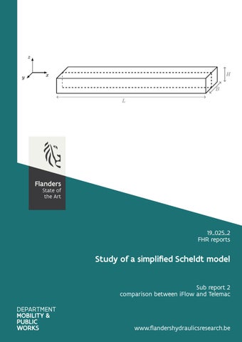
Cover figure
The Government of Flanders, Department of Mobility and Public Works, Flanders Hydraulics Research
Legal notice Flanders Hydraulics Research is of the opinion that the information and positions in this report are substantiated by the available data and knowledge at the time of writing. The positions taken in this report are those of Flanders Hydraulics Research and do not reflect necessarily the opinion of the Government of Flanders or any of its institutions. Flanders Hydraulics Research nor any person or company acting on behalf of Flanders Hydraulics Research is responsible for any loss or damage arising from the use of the information in this report. Copyright and citation The Government of Flanders, Department of Mobility and Public Works, Flanders Hydraulics Research, 2020 D/2020/3241/194 This publication should be cited as follows: <ĂƉƚĞŝŶ͕ ^͘:͖͘ ŝ͕ Y͖͘ ^ĐŚƌĂŵŬŽǁƐŬŝ͕ '͖͘ DŽƐƚĂĞƌƚ͕ &͘ (2020). Study of a simplified Scheldt model: Subreport 2: comparison between iFlow and Telemac. Version 2.0. FHR Reports, 19_025_2. Flanders Hydraulics Research: Antwerp Reproduction of and reference to this publication is authorised provided the source is acknowledged correctly. Document identification Customer:
Flanders Hydraulics Research
Ref.:
WL2020R19_025_2
Keywords (3‐5):
Idealized modelling, numerical simulations, Scheldt
Knowledge domains:
Hydraulics and sediment Tides Numerical modelling ‐ Hydraulics and sediment Water levels Numerical modelling
Text (p.):
18
Confidentiality:
No
Author(s):
Kaptein, S.J.; Bi, Q.
Appendices (p.):
0
Available online
Control Name Revisor(s):
Schramkowski, G.
Project leader:
Kaptein, S.J.
Signature Dr. George P. Schramkowski
Digitaal ondertekend door Dr. George P. Schramkowski Datum: 2020.11.26 12:49:59 +01'00' Getekend door: Steven Kaptein (Signature) Getekend op: 2020-11-30 10:45:19 +00:00 Reden: Ik keur dit document goed
Approval Head of division:
F‐WL‐PP10‐5 version 23 VALID AS FROM: 11/6/2020
Mostaert, F.
Getekend door: Frank Mostaert (Signature) Getekend op: 2020-11-27 09:49:06 +00:00 Reden: Ik keur dit document goed
Study of a simplified Scheldt model: Subreport 2: comparison between iFlow and Telemac
Abstract The objective of this report is to compare the results of two different modeling tools iFlow and Telemac. Each modeling tool is applied to an extremely simplified Scheldt model: a geometry with a rectangular cross‐section, a constant width and a constant depth. The main purpose of the study is to challenge the assumptions on which iFlow is based and to estimate the extend to which they influence the reliability of the results. The results show that it was not possible to determine a ratio of between the water depth and the amplitude of the M2 tide for which iFlow clearly fails to reproduce the results of Telemac, in the present flow configuration and for the present parameters. Additionally, no single parameter governing the differences between iFlow and Telemac has been identified. However, more data (i.e. number of simulations) is required to carry out a significant study about the differences between iFlow and Telemac and iFlow needs to be pushed to the limits in terms of the ratio between the water depth and the magnitude of the M2 tide.
Final version
WL2020R19_025_2
III
Study of a simplified Scheldt model: Subreport 2: comparison between iFlow and Telemac
Contents Abstract................................................................................................................... III List of Figures ............................................................................................................ VI List of Tables ............................................................................................................. VII 1 Introduction .........................................................................................................
1
2 The iFlow model .................................................................................................... 2.1 Governing equations ........................................................................................... 2.2 Resolution techniques .........................................................................................
2 2 3
3 The Telemac model ................................................................................................. 3.1 Governing equations ........................................................................................... 3.2 Bottom boundary condition ...................................................................................
5 5 5
4 Simulation set‐up ................................................................................................... 4.1 Computational domain and grid .............................................................................. 4.2 Simulation settings .............................................................................................
6 6 6
5 Results................................................................................................................ 7 5.1 Post‐processing of the Telemac simulations................................................................. 7 5.2 Convergence of the Telemac simulations .................................................................... 8 5.3 Comparison between iFlow and Telemac.................................................................... 11 5.4 Estuary averaged epsilon ...................................................................................... 14 5.5 Conclusion....................................................................................................... 16
Final version
WL2020R19_025_2
V
Study of a simplified Scheldt model: Subreport 2: comparison between iFlow and Telemac
List of Figures Figure 1 Figure 2 Figure 3
Sketch of the computational domain for the Scheldt model, simplified to a maximum. .......... Grid configuration near the seaward boundary. ........................................................ Magnitude of the M2 tide over the estuary computed for two different period numbers (left). Difference and relative difference between these two signals (right). The two chosen periods are the last period and the second last period of a 40 day simulation. Simulation for ℎ = 20m and 𝐴M2 = 1m. ............................................................................................. Figure 4 Magnitude of the M2 tide over the estuary computed for two different period numbers (left). Difference and relative difference between these two signals (right). The two chosen periods are the last period and the second last period of a 40 day simulation. Simulation for ℎ = 3m and 𝐴M2 = 1m. ............................................................................................. Figure 5 Convergence norm for simulations with different values of ℎ/𝐴M2 , ranging from ℎ/𝐴M2 = 3 to ℎ/𝐴M2 = 100. ........................................................................................... Figure 6 Difference between iFlow and Telemac results for a simulation with ℎ/𝐴M2 =20. .................. Figure 7 Difference between iFlow and Telemac results for a simulation with ℎ/𝐴M2 =3. ................... Figure 8 Difference norm for simulations with different values of ℎ/𝐴M2 . .................................... Figure 9 Evolution of the estuary averaged 𝜀 as a function of 𝜀. ................................................ Figure 10 Difference between iFlow and Telemac as a function of the estuary averaged 𝜀. ..................
VI
WL2020R19_025_2
6 6
8
9 10 11 12 13 14 15
Final version
Study of a simplified Scheldt model: Subreport 2: comparison between iFlow and Telemac
List of Tables Table 1
Parameter values for an idealized Scheldt model ........................................................
Final version
WL2020R19_025_2
6
VII
Study of a simplified Scheldt model: Subreport 2: comparison between iFlow and Telemac
1 Introduction The use of complex three‐dimensional models, such as Telemac, for studying estuaries has been a common practice over the last decades (Malcherek, 2000; Smolders et al., 2016). Their accurate implementation of the river geometry, the river bathymetry, the external forcing and the possibility of including tributaries or coastal regions make them an appreciated tool for investigating case studies. However, two of the major drawbacks of complex three‐dimensional models are (i) their lack of short computational time and (ii) the complex analysis of the results. These features make it almost impossible to investigate more than one or two scenarios or to give an interpretation of the results based on individual physical processes. Subsequently, the use of faster, idealized and process based models, such as iFlow, have become more and more popular over the last years (Brouwer et al., 2018; Brouwer et al., 2017; Dijkstra et al., 2017, 2019a,b). These models allow for the simulation of multiple scenarios (e.g. order of magnitude hundred to thousand) at reasonable computational costs. Additionally, the way iFlow is constructed allows for a decomposition of the different variables (i.e. water‐level, velocity fields, sediment concentrations) into the sum of individual contri‐ butions. Each of these contributions corresponds then to a specific physical mechanism. A major drawback is that iFlow uses a highly idealized representation of an estuary. For example, the bathymetry is smoothened and the model is width‐averaged. Some of the fundamental simplifying assumptions are not necessarily met (more detail about these assumptions in Section 2). In order to solve the drawbacks of each of the two models, a comparison is undertaken. This comparison will clarify the influence of some of the simplifying assumptions on iFlow’s results. While iFlow and Telemac are based on similar sets of equations, they adopt distinctive boundary conditions and fundamlentally different solution methods. Accordingly, rigorous choices are required and need to be motivated in order to bring iFlow and Telemac as close together as possible. These choices include the grid properties, model parameters and boundary conditions, and are detailed in Sections 2, 3 and 4. To identify and limit the number of discrepancies of the model, it was chosen to gradually increase the complexity of the study case by starting from the most simple case: a semi‐enclosed rectilinear tidal channel of rectangular cross‐section, with a constant depth and width, and forced at one end by an M2 and an M4 signal.
Final version
WL2020R19_025_2
1
Study of a simplified Scheldt model: Subreport 2: comparison between iFlow and Telemac
2 The iFlow model 2.1
Governing equations
The iFlow model solves the width‐averaged Saint‐Venant (or shallow water) equations for the conservation of momentum, as well as a width‐averaged continuity equation for the conservation of mass 𝑅+𝜁
𝜕𝑢 𝜕𝑢 𝜕𝑢 𝜕𝜁 1 𝜕𝜌 𝜕 𝜕𝑢 +𝑢 +𝑤 = −𝑔 − ∫ 𝑑𝑧 ̃ + (𝜈𝑇 ) , 𝜕𝑡 𝜕𝑥 𝜕𝑧 𝜕𝑥 𝜌ref 𝜕𝑥 𝜕𝑧 𝜕𝑧
(1a)
𝑧
𝜕𝑤 𝜕𝐵𝑢 𝐵 + = 0, 𝜕𝑧 𝜕𝑥
(1b)
in which 𝑢 and 𝑤 are the velocity variables, respectively along 𝑥 (along estuary coordinate), and along 𝑧 (vertical coordinate). The symbol 𝑡 represents time, 𝑔 the acceleration of gravity, 𝜁 the surface elevation, 𝑅 the mean level of the river surface, 𝜌ref the reference density, 𝜌 the density of the fluid, 𝜈𝑇 the eddy‐viscosity, 𝐻 the water depth and 𝐵 the channel width. The associated boundary conditions comprise a partial slip condition and a no‐penetration condition at the bed (i.e. 𝑧 = −𝐻), a no‐stress condition and a kinematic boundary condition at the surface (i.e. 𝑧 = 𝑅 + 𝜁), a time‐dependent tidal forcing at the seaward boundary (i.e. 𝑥 = 0) and an imposed river discharge at the landward boundary (i.e. 𝑥 = 𝐿). The equations for these boundary conditions are 𝜕𝑢 = 𝑠𝑓 𝑢 𝜕𝑧 𝜕𝐻 𝑤+𝑢 =0 𝜕𝑥 𝜕𝑢 𝜈𝑇 =0 𝜕𝑧 𝜕𝜁 𝜕𝜁 𝑤= +𝑢 𝜕𝑡 𝜕𝑥 𝜁 = 𝐴M2 cos(𝜎𝑡) + 𝐴M4 cos(2𝜎𝑡 + 𝜑) 𝜈𝑇
at 𝑧 = −𝐻,
(2a)
at 𝑧 = −𝐻,
(2b)
at 𝑧 = 𝑅 + 𝜁,
(2c)
at 𝑧 = 𝑅 + 𝜁,
(2d)
at 𝑥 = 0,
(2e)
at 𝑥 = 𝐿.
(2f)
𝑅+𝜁
𝐵 ∫ 𝑢𝑑𝑧 = −𝑄 −𝐻
Several new parameters appear: 𝑠𝑓 , the friction coefficient, 𝐴M2 and 𝜎, respectively the amplitude and the frequency of the M2 tide, 𝐴M4 , the amplitude of the M4 tide, and 𝑄 the river discharge, and 𝜑 the phase of the M4 tide. It is possible to derive an equation for the surface elevation by integrating Eq. (1b) over the depth and to use Eqs (2b) and (2d), 𝑅+𝜁
𝜕𝜁 𝜕 ⎛ ⎞ ⎜ 𝐵 + ⎜𝐵 ∫ 𝑢𝑑𝑧 ⎟ ⎟=0 𝜕𝑡 𝜕𝑥 ⎝ −𝐻 ⎠ 2
WL2020R19_025_2
(3)
Final version
Study of a simplified Scheldt model: Subreport 2: comparison between iFlow and Telemac
2.2
Resolution techniques
The resolution technique for solving Eqs (1a), (3) relies on the linearization of the equations. By making the equations non‐dimensional using 𝐿 for 𝑥, 𝐻 for the 𝑧, 𝐴M2 for 𝜁 and 𝜎 for 𝑡, it is possible to show that the non‐linear advection terms scale with 𝜀 = 𝐴M2 /𝐻 (see Brouwer et al., 2017 for more details). If we assume that the baroclinic term also scales with 𝜀 and that 𝜀 ≪ 1, the solution can take the form of a series in which the variables are decomposed as 𝑢 = 𝑢 0 + 𝑢1 + 𝑢2 + ⋯ , 𝑤 = 𝑤 0 + 𝑤1 + 𝑤 2 + ⋯ , 𝜁 = 𝜁 0 + 𝜁 1 + 𝜁2 + ⋯ with 𝑢1 /𝑢0 ∼ 𝜀, 𝑢2 /𝑢1 ∼ 𝜀 and 𝜀 ≪ 1 (and similarly for 𝑤 and 𝜁). Accordingly, it is possible to split the governing equations and the associated boundary conditions into a set of equations governing the leading order variables and a set of equations governing the first order variables. At leading order, this decomposition gives 𝜕 𝜕𝑢0 𝜕𝜁 𝜕𝑢0 − (𝜈 ) = −𝑔 0 , 𝜕𝑡 𝜕𝑧 𝑇 𝜕𝑧 𝜕𝑥
(4a)
𝑅
𝜕𝜁 𝜕 ⎛ ⎞ = 0, ⎜ 𝐵 0+ ⎜𝐵 ∫ 𝑢0 𝑑𝑧 ⎟ ⎟ 𝜕𝑡 𝜕𝑥 ⎝ −𝐻 ⎠ 𝜕𝐵𝑢0 𝜕𝑤 = 0, 𝐵 0+ 𝜕𝑧 𝜕𝑥
(4b) (4c)
for the governing equations, and 𝜕𝑢0 𝜕𝑧 𝜕𝐻 𝑤0 + 𝑢 0 𝜕𝑥 𝜕𝑢0 𝜈𝑇 𝜕𝑧 𝜁0 𝜈𝑇
= 𝑠 𝑓 𝑢0
at 𝑧 = −𝐻,
(5a)
=0
at 𝑧 = −𝐻,
(5b)
=0
at 𝑧 = 𝑅,
(5c)
= 𝐴M2 cos(𝜎𝑡)
at 𝑥 = 0,
(5d)
at 𝑥 = 𝐿,
(5e)
𝑅
𝐵 ∫ 𝑢0 𝑑𝑧 = 0 −𝐻
for the boundary conditions. At first order the decomposition leads to 𝑅
𝜕𝑢1 𝜕 𝜕𝑢1 𝜕𝜁 1 𝜕𝜌0 𝜕𝑢 𝜕𝑢 − (𝜈 )=−𝑔 1 −∫ 𝑑 𝑧 ̃ − 𝑢 0 0 − 𝑤0 0 , 𝜕𝑡 𝜕𝑧 𝑇 𝜕𝑧 𝜕𝑥 𝜌ref 𝜕𝑥 𝜕𝑥 𝜕𝑧
(6a)
𝑧
𝑅
𝜕 ⎛ 𝜕𝜁 ⎞ − 𝜕 (𝐵 𝑢 | 𝜁 ) , ⎜ 𝐵 1 =− ⎜𝐵 ∫ 𝑢1 𝑑𝑧 ⎟ ⎟ 0𝑅 0 𝜕𝑡 𝜕𝑥 𝜕𝑥 ⎝ −𝐻 ⎠ 𝜕𝑤1 𝜕𝐵𝑢1 𝐵 =− , 𝜕𝑧 𝜕𝑥
Final version
WL2020R19_025_2
(6b) (6c)
3
Study of a simplified Scheldt model: Subreport 2: comparison between iFlow and Telemac for the governing equations, and 𝜕𝑢1 𝜕𝑧 𝜕𝐻 𝑤1 + 𝑢 1 𝜕𝑥 𝜕𝑢1 𝜈𝑇 𝜕𝑧 𝜁1 𝜈𝑇
=𝑠𝑓 𝑢1
at 𝑧 = −𝐻,
(7a)
=0
at 𝑧 = −𝐻,
(7b)
at 𝑧 = 𝑅,
(7c)
at 𝑥 = 0,
(7d)
at 𝑥 = 𝐿,
(7e)
𝜕 𝜕𝑢 (𝜈𝑇 0 ) 𝜕𝑧 𝜕𝑧 =𝐴M4 cos(2𝜎𝑡 + 𝜑) = − 𝜁0
𝑅
∫ 𝑢1 𝑑𝑧 = −
𝑄1 − 𝑢0|𝑅 𝜁0 𝐵
−𝐻
for the boundary conditions. As mentioned previously, this decomposition linearizes the equations. Subsequently, superposition techniques can be applied (i.e. solution of the sum is equal to the sum of the solution). It is this technique that allows to consider different forcing mechanism independently of the others. The last characteristic assumption of iFlow is the harmonic decomposition. The harmonic decomposition implies that only the steady state solution is solved and that: 𝜕 𝑢̂0 = i𝜎𝑢̂0 𝜕𝑡 𝜕 𝑢̂1 = 2i𝜎𝑢̂1 𝜕𝑡 with 𝑢̂ the complex velocity associated to 𝑢. The same decomposition applies to 𝑤 and 𝜁. As a result, the leading order variables evolve with the M2 tidal frequency while the first order variable evolve with the M4 tidal frequency but also have a residual component. Depending on the numerical settings, iFlow can solve the first and leading order equations (semi‐)analytically or numerically. For more information about the solving procedures, the reader is referred to the literature (Dijkstra, 2017; Dijkstra et al., 2017). To summarize, the three major assumption of iFlow that are not necessarily present in Telemac are 1. the tidal amplitude is much smaller than the water depth 2. the baroclinic term only appears at first order (weak horizontal density gradient) 3. the time evolution is periodic with harmonic equal to the M2 tidal frequency and the M4 tidal frequency In the present report, we will focus on assumption 1 by performing 27 different simulations, each with a differ‐ ent depth. In each simulation the amplitude of the M2 and M4 amplitude are kept small, such that a difference in water depth results immediately in a different ratio between tidal amplitude and the constant water‐depth. Simultaneously, any standard error not related to this ratio could also challenge assumption 3. It is import‐ ant to not that the standard bottom boundary condition implemented in Telemac is a quadratic friction law. However, in order to have consistency between iFlow and Telemac, the linear friction law of iFlow has been implemented in Telemac.
4
WL2020R19_025_2
Final version
Study of a simplified Scheldt model: Subreport 2: comparison between iFlow and Telemac
3 The Telemac model 3.1
Governing equations
This section is entirely taken over from Bi et al., 2020 The hydrodynamics in Telemac‐3D is modeled with 3D incompressible Reynolds‐averaged Navier‐Stokes equa‐ tions. The Navier–Stokes equations for incompressible flows consist of two equations: the continuity and the momentum equations. Assuming that fluid density is incompressible, and applying the Boussinesq ap‐ proximation to the Reynolds stress term, the mass and momentum conservation equations under vector form read: ∇⋅u=0
(8)
𝜕u 1 + (u ⋅ ∇)u = − ∇𝑝 + ∇ ⋅ [(𝜈 + 𝜈𝑇 ) ∇u] + g + F (9) 𝜕𝑡 𝜌 where ∇ is the gradient operator, u is the Reynolds‐averaged mean velocity vector, 𝑡 is the time, 𝜌 is the fluid density, 𝑝 is the mean pressure, 𝜈 is the kinematic viscosity of the fluid, 𝜈𝑇 is the turbulence eddy viscos‐ ity, g is the gravitational force vector and F is the vector containing other external forces, e.g. Coriolis force and centrifugal force. In many industrial and environmental flows, the density of the carrying phase is not a constant but varies as a function of the temperature, salinity and/or sediment concentration. The buoyancy effects due to the density gradient thus should be included in the governing equations in order to model the stratification properly. The varying density could be included in the Eq. (8) and Eq. (9). But there is also an alternative way that enables the treatment of buoyancy effect by means of the gravity term if the change of density Δ𝜌/𝜌 < 0.1). Based on this assumption, an extra term representing the buoyancy force can be derived and added into the momentum equation. The details can be found in the Telemac‐3D theory guide. To the governing equations, the turbulence eddy viscosity 𝜈𝑇 has to be closed with a turbulence model. However, in this project, the eddy‐viscosity was taken constant.
3.2
Bottom boundary condition
One of the major differences between iFlow and Telemac resides in the bottom boundary condition. First iFlow assumes a partial slip condition with a linear formulation of the velocity dependence of the stresses at the bottom. Telemac uses a quadratic formulation. Second, in iFlow, the boundary condition is really applied at the bottom, while in Telemac the boundary condition is applied at the center of the first cell above the bottom. If we note Δ𝑧 the distance of the first cell center from the bottom wall, the application of a partial slip boundary condition is formulated as 𝜕𝑢 𝜈𝑇 = 𝑠𝑓 𝑢 at 𝑧 = −𝐻 + Δ𝑧. (10) 𝜕𝑧 Using a Taylor series development of Eq. (10) at 𝑧 = −𝐻 + Δ𝑧 gives 𝜕 𝜕𝑢 𝜕 𝜕𝑢 + Δ𝑧 (𝜈 ) = 𝑠𝑓 𝑢 + Δ𝑧 (𝑠 𝑢) + 𝑂 (Δ𝑧 2 ) at 𝑧 = −𝐻 + Δ𝑧, (11) 𝜈𝑇 𝜕𝑧 𝜕𝑧 𝑇 𝜕𝑧 𝜕𝑧 𝑓 which is different from the formulation in iFlow (see Eq. (2a)). In other words, applying the partial slip bound‐ ary at 𝑧 = −𝐻 + Δ𝑧 instead of 𝑧 = −𝐻 gives an error of 𝜕 𝜕𝑢 (𝑠𝑓 𝑢 − (𝜈𝑇 )) , Δ𝑧 (12) 𝜕𝑧 𝜕𝑧 which can be controlled by refining the grid close to the bottom boundary.
Final version
WL2020R19_025_2
5
Study of a simplified Scheldt model: Subreport 2: comparison between iFlow and Telemac
4 Simulation set‐up 4.1
Computational domain and grid
As mentioned in the earlier sections, the model is kept as simple as possible in the first instance before being complexified gradually. We start with a semi‐enclosed rectilinear channel of constant rectangular cross‐section for the idealized Scheldt geometry. This set‐up is sketched in Fig. 1 by the solid lines. Since iFlow is width‐ averaged, i.e. two‐dimensional‐vertical, the computation domain is rectangular and sketched by the dashed lines. Figure 1 – Sketch of the computational domain for the Scheldt model, simplified to a maximum.
𝑧
𝑦
𝐻
𝑥 𝐵 𝐿
Since iFlow is a width‐averaged model and Telemac not, different choices are possible for the horizontal grid‐ cell distribution in Telemac. We choose a regular triangulated grid as displayed in Fig 2. Figure 2 – Grid configuration near the seaward boundary.
4.2
Simulation settings
The settings used in the different simulations are summarized in Table 1. In this table the phase of the M4 tide at 𝑥 = 0, i.e. 𝜑Mℎ is also given. Table 1 – Parameter values for an idealized Scheldt model
6
𝐿 (km)
𝐵 (m)
𝐴M2 (m)
𝐴M4 (m)
𝜑Mℎ (rad)
Q1 (m3 s−1 )
𝜈𝑇 (m2 s−1 )
𝑠𝑓 (m3 s−1 )
160
500
1.0
0.1
0
36
0.0367
0.0048
WL2020R19_025_2
Final version
Study of a simplified Scheldt model: Subreport 2: comparison between iFlow and Telemac
5 Results 5.1
Post‐processing of the Telemac simulations
Since iFlow and Telemac differ in their method of solving the governing equations, some post‐processing is required before comparing the results. On the one hand, iFlow provides the water level, and the velocities under the form of an M2 and an M4 signal, each characterized by an amplitude and a phase as a function of the 𝑥 position (and the 𝑧 position for the depth). On the other hand, Telemac provides the instantaneous value of the water level and the velocity over the entire domain, at specific time steps. It was chosen to extract the M2 signals M4 from the Telemac data to perform a direct comparison with the iFlow output. This extraction requires a specific protocol: • At each grid point, a time‐series of the water‐level and the velocity is recorded. • For each time‐series, a specific M2 tidal period is selected that is not influenced by the spin‐up of the simulation. • The data available for this period is interpolated on an equidistant temporal grid, in such a way that one period contains exactly an integer number of time‐steps. • A fast Fourrier transform is applied to the interpolated data which gives the amplitudes and phases for M2, M4 and higher order frequencies. • Finally, a spatial distribution of the amplitudes and phases for the different frequencies is reconstructed. In this protocol, the size of the Telemac data (several Gb) caused the initial scripts to be very time consuming (several hours to process one simulation). Accordingly, some time was allocated (and spent) in order to op‐ timize the scripts. They currently run in a couple of tens of seconds. A second challenge that emerged, was the estimation of the convergence time in Telemac. It was chosen to simulated 40 days (approximately 75 tidal periods), which took between 6 to 7 hours on a laptop.
Final version
WL2020R19_025_2
7
Study of a simplified Scheldt model: Subreport 2: comparison between iFlow and Telemac
5.2
Convergence of the Telemac simulations
In practice, it was found that convergence was not reached within the 40 days simulation time for all the configurations tested. To backup‐up this statement, it is important to clarify the convergence criteria. It is assumed that convergence is reached locally when the relative error 𝜂𝜓 , locally defined as, 𝜂𝜓 (𝑥) = ∣
𝜓𝑖 (𝑥) − 𝜓𝑖+1 (𝑥) ∣ 𝜓(𝑥)
(13)
is smaller than at least 𝜀2 all over the estuary. Arbitrary, we set then maximum tolerated relative error to 10−3 . In Eq. (13), 𝜓 refers to a quantity such as a time‐series, the amplitude along the estuary or the phase along the estuary. The subscript 𝑖 refers to a specific period. The threshold value of 10−3 might seem very small. However, to carry out a meaningful comparison, the error due to the lack of convergence needs to be negligible with respect to the relative difference between iFlow results and Telemac results. Simulating 40 days (or 75 tidal periods) in Telemac on one processor took between 6 or 7 hours (wall time). As a result, a crucial step in this protocol is to determine the number of periods after which the simulation is converged. Ideally, as few periods as possible should be simulated in order reduce significantly computation time and stored data. However, the number of periods is difficult to estimate since the number of periods after which convergence is obtained varies considerably with the set‐up. This phenomenon is illustrated in Figs 3 and 4, by means of the relative error 𝜀𝜓 and the absolute error, 𝜂𝜓𝑎 (𝑥) = |𝜓𝑖 (𝑥) − 𝜓𝑖+1 (𝑥)|. For a ratio ℎ/𝐴M2 = 20 (Fig. 3), the absolute difference in M2 tide amplitude between two successive periods is of the order of 10−7 m over the estuary. The relative difference is of order 1.0×10⁻⁷ %. These results indicate a satisfying convergence. Figure 3 – Magnitude of the M2 tide over the estuary computed for two different period numbers (left). Difference and relative difference between these two signals (right). The two chosen periods are the last period and the second last period of a 40 day simulation. Simulation for ℎ = 20m and 𝐴M2 = 1m.
In contrast, for a ratio ℎ/𝐴M2 = 3 (Fig. 4), the relative difference if M2 tide amplitude between two successive periods is almost of order 10% towards the landwards side of the estuary. Nevertheless, the absolute error is still of order 10−7 m. Additionally, the amplitude in the M2 tidal signal is very small towards the landward side of the estuary. These two observations indicate that the small tidal amplitude provokes a slow convergence of
8
WL2020R19_025_2
Final version
Study of a simplified Scheldt model: Subreport 2: comparison between iFlow and Telemac the relative error in the M2 tidal signal, such that a longer simulation period might be required for a simulation with ℎ/𝐴M2 = 3 in the present configuration. Figure 4 – Magnitude of the M2 tide over the estuary computed for two different period numbers (left). Difference and relative difference between these two signals (right). The two chosen periods are the last period and the second last period of a 40 day simulation. Simulation for ℎ = 3m and 𝐴M2 = 1m.
To compare the convergence rate in between the simulations, we define a norm 𝑁𝜂,𝜓 by averaging the error 𝜂𝜓 over the estuary according to 𝐿 1 𝑁𝜀,𝜓 = ∫ 𝜂𝜓 (𝑥)𝑑𝑥. (14) 𝐿 0 In Eq. (14), the norm operator is applied to the relative error, but the norm for the absolute error is defined by the same operator. The order of magnitude of 𝑁𝜂,|𝜁0 | and 𝑁𝜂,|𝜁1 | for the convergence is shown in Fig 5 for different values of ℎ/𝐴M2 . From this figures, it appears that: (i) the absolute error is of order 10−7 m for all the tested values of ℎ/𝐴M2 , and for the both the M2 signal and the M4 signal; (ii) the relative error is approximately one order of magnitude larger for the M4 signal than for the M2 signal (which makes sence since the relative error is normalized by the tidal signal and the M4 tidal signal has a smaller amplitude than the M2 tidal signal); (iii) the simulation with ℎ/𝐴M2 = 3 is only with a significantly larger magnitude of the norm of the relative error, suggesting convergence was not reached yet. This latter observation is strange since a smaller depth means increased friction, thus a shorter time to reach the stationary solution.
Final version
WL2020R19_025_2
9
Study of a simplified Scheldt model: Subreport 2: comparison between iFlow and Telemac Figure 5 – Convergence norm for simulations with different values of ℎ/𝐴M2 , ranging from ℎ/𝐴M2 = 3 to ℎ/𝐴M2 = 100.
10
WL2020R19_025_2
Final version
Study of a simplified Scheldt model: Subreport 2: comparison between iFlow and Telemac
5.3
Comparison between iFlow and Telemac
The difference between the iFlow results and the Telemac results is shown in Figs 6 and 7 for two different val‐ ues of the ℎ/𝐴M2 ratio. Clearly, the amplitude and the phase of the M2 and the M4 tide overlap for ℎ/𝐴M2 =20 (see Fig. 6). However, for ℎ/𝐴M2 =3, some small descrepancies are noticible in the amplitudes and some more significant difference are observable in the phases (see Fig. 7). Figure 6 – Difference between iFlow and Telemac results for a simulation with ℎ/𝐴M2 =20.
To estimate the influence of the ratio ℎ/𝐴M2 on the difference between the results computed by iFlow and the results computed by Telemac, we introduce the relative difference 𝐸𝜓 . This relative difference is analogous to
Final version
WL2020R19_025_2
11
Study of a simplified Scheldt model: Subreport 2: comparison between iFlow and Telemac Figure 7 – Difference between iFlow and Telemac results for a simulation with ℎ/𝐴M2 =3.
the relative error 𝜀𝜓 and is defined as 𝐸𝜓 (𝑥) = ∣
𝜓𝑇 𝑒 (𝑥) − 𝜓𝑖𝐹 (𝑥) ∣. 𝜓𝑇 𝑒 (𝑥)
(15)
In Eq. (15), 𝜓 still refers to a physical quantity. The absolute difference would be defined as, 𝐸𝜓𝑎 (𝑥) = |𝜓𝑇 𝑒 (𝑥) − 𝜓𝑖𝐹 (𝑥)|. Analogy with Eq. (14), we define the norm of the relative difference 𝐿
𝑁𝐸,𝜓 =
1 ∫ 𝐸𝜓 (𝑥)𝑑𝑥. 𝐿 0
(16)
The norm of the absolute difference does not show a clear trend with ℎ/𝐴M2 (see Fig. 8). Nevertheless, the norm of the relative difference is the highest for the low values of the ℎ/𝐴M2 ratio, suggesting that for these 12
WL2020R19_025_2
Final version
Study of a simplified Scheldt model: Subreport 2: comparison between iFlow and Telemac values of ℎ/𝐴M2 , the iFlow assumptions start to be challenged. However, these values also correspond to the simulations for which convergence is still disputed, although the values of 𝑁𝜀,𝜓 (measure of the convergence) are significantly smaller than the value for 𝑁𝐸,𝜓 (measure of the difference). Figure 8 – Difference norm for simulations with different values of ℎ/𝐴M2 .
A peculiar feature of the evolution of the 𝑁𝐸,𝜓 norm, is that there is no steady dependence on ℎ/𝐴M2 . This phenomenon could be related to the quality of the ℎ/𝐴M2 ratio as a measure for 𝜀. Indeed, as can be seen in Figs 3 and 7, the damping of the tidal amplitude for ℎ/𝐴M2 is relatively fast, which implies that the 𝜀 becomes very small in a relatively short distance from the mouth, even if it is large at the mouth itself.
Final version
WL2020R19_025_2
13
Study of a simplified Scheldt model: Subreport 2: comparison between iFlow and Telemac
5.4
Estuary averaged epsilon
To overcome the shortcoming of the 𝜀 criterion, it is possible to define an average 𝜀, 𝜀 as 𝐿 𝐴M2 (𝑥) 1 ∫ 𝑑𝑥 𝐿 0 ℎ(𝑥)
(17)
𝐿 𝐴M4 (𝑥) 1 𝜀= ∫ 𝑑𝑥 𝐿 0 𝐴M2 (𝑥)
(18)
𝜀= for ℎ/M2 , and
for M2 /M4 . The evolution of 𝜀 as a function of ℎ/𝐴M2 is shown in Fig. 9. It becomes clear from this Figure, that there is no linear relationship between 𝜀 and 𝜀. A maximum seems to be reached around ℎ/𝐴M2 = 25, which is close to the resonance depth. More important, low values high values of 𝜀 do not necessarily coincide with large values of ℎ/𝐴M2 . Since the relationship between the norm of the difference between iFlow and Telemac Figure 9 – Evolution of the estuary averaged 𝜀 as a function of 𝜀.
and ℎ/𝐴M2 appears weak, it is interesting to investigate if the relationship between the norm of the difference between iFlow and Telemac and |𝜀| is more pronounced. As a result, the norm of the difference between iFlow and Telemac is displayed in Fig. 10. However, such a relationship does not appear clearly. These results imply that the differences between iFlow and Telemac can not be estimated via a single parameter ℎ/𝐴M2 or |𝜀|, but are governed by a more complex interplay between water‐depth, resonance and friction.
14
WL2020R19_025_2
Final version
Study of a simplified Scheldt model: Subreport 2: comparison between iFlow and Telemac Figure 10 – Difference between iFlow and Telemac as a function of the estuary averaged 𝜀.
Final version
WL2020R19_025_2
15
Study of a simplified Scheldt model: Subreport 2: comparison between iFlow and Telemac
5.5
Conclusion
Based on the results shown in the present report, we can draw the following conclusions: • In the tested configuration, it was not possible to determine a ratio of ℎ/𝐴M2 at which iFlow clearly fails at reproducing the results of Telemac • No single parameter governing the differences between iFlow and Telemac has been identified Furthermore, we suggest that any follow up study should tackle the following challenges • More data (i.e. number of simulations) is required to carry out a significant study about the differences between iFlow and Telemac • iFlow needs to be pushed to the limits in terms of ℎ/𝐴M2 ratio but also in terms of the average ratio ℎ/𝐴M2 (i.e., 𝜀) • A method to overcome or at least reduce the transient period in Telemac is necessary to shorten com‐ putational time and to limit data output from a single Telemac simulation The results of iFlow and Telemac for the present configuration agree very well. However, due to the choices for the parameter values, the models have not yet been thouroughly challenged. Indeed, it was chosen to vary the 𝐴M2 /𝐻 by keeping 𝐴M2 constant and varying 𝐻. This method allow to maintain the same value of 𝐴M4 /𝐴𝑀 𝑡 for all the simulations. However, by varying 𝐻, we also varied the amount of friction, which caused the tidal wave to be rapidly damped for low value of 𝐴M2 /𝐻. These were the value for which the largest difference between the Telemac and iFlow were expected, but due to the damping, the hypothesis 𝐴M2 /𝐻 ≪ 1 was still valid in the upper estuary. In the lower estuary, this hypothesis was challenged, but the water‐level was imposed at the seaward boundary. As a result, the expected differences between iFlow and Telemac did not occur. In a follow‐up study, it is strongly adviced to vary the 𝐴M2 /𝐻 by keeping 𝐻 constant and vary both 𝐴M2 and 𝐴M4 simultaneously such that 𝐴M4 /𝐴M2 remains constant. In this way, only the 𝐴M2 /𝐻 ratio varies, like in the present study, but friction should not affect the outcome of the comparison. The present plots, displaying the difference between iFlow and Telemac as a function of 𝐴M2 /𝐻 could then be reproduced. The convergence of the Telemac simulation can subsequently be checked by repeating the graphs using the Telemac results after a different number of oscillations. These results could be compared to Telemac results for which the initial condition are the iFlow results, to see if the convergence time decreases. The convergence criterium should be based on the difference in value between two successive periods, compared to the local value of 𝜀. To finish the procedure should be reiterated by varying 𝐻, keeping both 𝐴M2 /𝐻 and 𝐴M4 /𝐴M2 constant. It is recomended to focus on parameter values lying in different regimes, e.g. a value of 𝐻 for which strong damping occurs, and a value of 𝐻 for which resonance occurs.
16
WL2020R19_025_2
Final version
Study of a simplified Scheldt model: Subreport 2: comparison between iFlow and Telemac
References Bi, Q.; Kaptein, S.; Schramkowski, G.; Smolders, S.; Mostaert, F. (2020). The iFlow inspired TELEMAC‐3D model. Sub report 1 – Comparing ETM dynamics with the iFlow model. WL Rapporten, WL2020R19_025_1. Flanders Hydraulics Research: Antwerp, Belgium Brouwer, R. L.; Schramkowski, G. P.; Dijkstra, Y. M.; Schuttelaars, H. M. (2018). Time Evolution of Estuar‐ ine Turbidity Maxima in Well‐Mixed, Tidally Dominated Estuaries: The Role of Availability‐and Erosion‐Limited Conditions. Journal of Physical Oceanography 48 (8): 1629–1650 Brouwer, T.; Schramkowski, G.; Mostaert, F. (2017). Geïdealiseerde processtudie van systeemovergangen naar hypertroebelheid. 2.0. WL Rapporten, 13_103_3. Flanders Hydraulics Research: Antwerp, Belgium Dijkstra, Y. M. (2017). iFlow modelling framework. User manual & technical description. Dijkstra, Y. M.; Brouwer, R. L.; Schuttelaars, H. M.; Schramkowski, G. P. (2017). The iFlow modelling frame‐ work v2. 4: a modular idealized process‐based model for flow and transport in estuaries. Geoscientific Model Development 10 (7): 2691–2713 Dijkstra, Y. M.; Schuttelaars, H. M.; Schramkowski, G. P. (2019a). A Regime Shift From Low to High Sediment Concentrations in a Tide‐Dominated Estuary. Geophysical Research Letters 46 (8): 4338–4345 Dijkstra, Y. M.; Schuttelaars, H. M.; Schramkowski, G. P.; Brouwer, R. L. (2019b). Modeling the Transition to High Sediment Concentrations as a Response to Channel Deepening in the Ems River Estuary. 124 (3): 1578– 1594 Malcherek, A. (2000). Application of TELEMAC‐2D in a narrow estuarine tributary. 14 (13): 2293–2300 Smolders, S.; Maximova, T.; Vanlede, J.; Plancke, Y.; Verwaest, T.; Mostaert, F. (2016). Integraal Plan Boven‐ zeeschelde: Subreport 1 – SCALDIS: a 3D Hydrodynamic Model for the Scheldt Estuary. 5.0. WL Rapporten, 13_131. Flanders Hydraulics Research: Antwerp, Belgium
Final version
WL2020R19_025_2
17
DEPARTMENT MOBILITY & PUBLIC WORKS Flanders hydraulics Research Berchemlei 115, 2140 Antwerp T +32 (0)3 224 60 35 F +32 (0)3 224 60 36 waterbouwkundiglabo@vlaanderen.be www.flandershydraulicsresearch.be