

Superconductivity and the emerging Field oF “twiStronicS”
Layla Shaffer ’22
In 2018, Physicists at MIT observed that when two layers of graphene are stacked and twisted at a “magic angle” of 1.56 degrees, the bilayer is transformed into a superconductor–a material that conducts electricity with zero resistance or energy waste. Superconductivity has vast implications, from high-speed magnetic levitation trains to alternative energy systems. Though minute in scale, simply changing the angle of stacked graphene (graphene is a single layer of carbon atoms that is 200 times stronger than steel) has revolutionized the field of twistronics, creating vital ramifications in the ever-evolving race of nano-technology. The problem with the twister graphene-bilayer, and other superconductors in general, is that they only function at extremely cold temperatures. Temperatures around absolute zero allow a low energy state in which electrons overcome their repulsion to form Cooper Pairs–the key to the lack of resistance in superconductivity. Any superconductors that are able to operate at slightly higher temperatures (like H₃S at -94 degrees Fahrenheit) require extreme amounts of pressure. Thus, research involving superconductors that can operate at higher temperatures with manageable amounts of pressure would advance our understanding of condensed-matter physics and have resounding consequences in society and technology.
Fast forward three years later, the same MIT research group discovered magic-angle twisted trilayer graphene (MATTG), which accomplished this new goal of twistronics. Based on their work with the graphene bilayer, the researchers hypothesized that they could stack three sheets of graphene and twist the middle layer to the magic angle, creating a symmetrical lattice structure to cause the electrons to pair up. The structure–just a few micrometers wide and three atoms tall–had electrodes attached to either end with an electric current running through. They measured that zero energy dissipated, meaning that the MATTG was indeed a superconductor. Not only did the cutting-edge “graphene sandwich” con-
firm the 1.56-degree value of the magic angle in a structure with more than two layers, but it exhibited better electron structure turnability and superconducting properties than its bilayer counterpart. Moreover, the three layers of MATTG allowed scientists to create parameters for graphene’s superconductive properties by applying varying amounts of an external electric field. In doing so the researchers created ultra-strongly coupled superconductivity, a phenomenon rarely seen before. Researchers also found that MATTG had a relatively high critical temperature of around 3 Kelvins even when there was low electron density.
The results reveal the discovery of the strongest-coupled superconductor currently known. Its tunability will allow for future twistronic systems to be studied in greater depth and has a plethora of applications for quantum information technologies. Most importantly, the tunability of the trilayer will allow scientists to explore the underlying mechanisms of superconductivity, setting the stage for multi-layer graphene stacks that can operate in temperatures close to room temperature. From magnetic levitation trains to high-energy particle accelerators, the discovery and confirmation of 1.56° yields endless new paths of discovery.
References
Chu, J. (2021). Physicists create tunable superconductivity in twisted graphene “nanosandwich”. Retrieved 19 April 2022, from https://news.mit.edu/2021/ physicists-create-tunable-superconductivity-twisted-graphene-nanosandwich-0201
criSpr FoodS: what are they?
Kiley Alt ’23
CRISPR stands for Clustered Regularly Interspaced Short Palindromic Repeats, the bacterial defense system that is the basis of CRISPR-Cas9 genome editing. The CRISPR-Cas9 system is a new way to genetically modify anything from foods to animals. The “Cas9” refers to the enzyme that “cuts out” the targeted gene. CRISPR editing has three steps: disruption, deletion, and insertion or correction. The CRISPR system “spacer sequences” are encoded into a strand of RNA (crRNA), which guides the system to the targeted DNA sequence. When attached to the DNA strand, the Cas9 enzyme removes the targeted DNA sequence from the strand. Then, the remaining two pieces of DNA can either be inserted or a new section of DNA can be inserted between the original two strands. The goal of the CRISPR method is to modify an organism’s genome without introducing foreign DNA. This is what differentiates CRISPR editing from the standard GMO (genetically modified organism), which introduces a specific gene from another species into the subject organism. This process can lead to the subject organisms’ cells either rejecting the DNA or accepting the DNA and possibly mutating in the process.
Government decisions on CRISPR-Cas9 edited foods’ availability in grocery stores remain controversial. Given that both common GMOs and CRISPR-edited foods require the use of marking genes in the positive selection process, governments are torn as to whether CRISPR edited foods are any better for the public than

common GMOs. Furthermore, debate on the legality of testing CRISPR-Cas9 genome editing on animals complicates the issue. Many people support CRISPR-Cas9 testing on animals in hopes of the technology being introduced to humans. If this were to happen, CRISPR-Cas9 would change modern medicine in drastic ways, as modifying human genomes could permanently change generations as edited DNA is passed down to offspring. While the idea of altering a human’s genetic makeup comes with many legal and ethical questions, CRISPR editing could eliminate many hereditary conditions from burdening future generations, possibly eliminating some altogether.
References
“CRISPR/Cas9.” CRISPR, CRISPR Therapeutics, http:// www.crisprtx.com/gene-editing/crispr-cas9.
“Questions and Answers about CRISPR.” Broad Institute, Broad Institute, 4 Aug. 2018, https://www. broadinstitute.org/what-broad/areas-focus/project-spotlight/questions-and-answers-about-crispr.
Shew, Aaron M., et al. “CRISPR versus GMOs: Public Acceptance and Valuation.” Global Food Security, Elsevier, 9 Nov. 2018, https://www.sciencedirect. com/science/article/pii/S2211912418300877.
the general adverSarial network: creating the realiStic Fake Sean Wu ’23
In February 2019, “thispersondoesnotexist.com” took the internet by storm. With every reload, a new, human, face appeared. The faces generated do not belong to real people—they are, rather, a combination of existing traits to produce an artificial identity—generated by an AI algorithm called General Adversarial Network (GAN).
GAN was created in 2014 by Ian Goodfellow, former member of the Google Brain Team who devised the idea of two neural networks collaborating to learn how to draw. After developing a primitive model, Goodfellow and colleagues published a paper that proposes a framework consisting of two competing neural network models, a Generator and a Discriminator. In GAN, the Discriminator is trained to recognize real images while the Generator tries to fool the Discriminator by fabricating fake images (Serpa, 2021).
In “thispersondoesnotexist.com”, the Discriminator is first trained with thousands of real images of people to tune its parameters, or decision making factors, to recognize real people. The image recognition is accomplished through a convolutional neural network modeled after visual cortex neurons that extracts important features and contours, such as the shape of the mouth and the texture of the eyebrows. Once the Discriminator completes its training, the Generator begins to create fake images of people’s faces by pulling together and transforming compressed data. Initially, the images generated deviate significantly from the resemblance of actual human faces. However, the Generator improves itself through a mathematical technique of back propagation. In fact, the GAN, like other neural networks, can be represented by a single, complex, and evolving math function. By adjusting the thousands of constants, or parameters, in the math function and finding the maximum in a multi-dimensioned graph, one can make the image output increasingly closer to a realistic image (Goodfellow, 2014).
The brilliance of the GAN framework lies in its ability to connect supervised and unsupervised machine
learning. Supervised learning uses labeled datasets to guide algorithms to classify data and predict outcomes, whereas unsupervised learning analyzes and clusters data to discover hidden patterns. GAN frames the unsupervised pattern recognition in real images as a supervised classification between real and fake images, breaking the barrier between two distinct applications of machine learning.
More recently in 2019, Nvidia AI engineers reported a breakthrough in their paper on StyleGAN. Since GAN involves compressing and decompressing an image to extract its features, the researchers tweaked low levels of the image compression process to control specific high-leveled details (Delua, 2021). StyleGAN can target and modify specific facial features in images, which is used in video editing and image fabrication.
While GAN technology is very useful in the machine learning, advertisement, and entertainment industries, its rise led to substantial ethical concerns as well. Since GAN can be used to fabricate realistic images, texts, and voices, it is no surprise that an extremely controversial branch called DeepFake emerged. While DeepFakes are useful for the entertainment industry and business marketing commercials, manipulating an audience to believe in a fraudulent reality is dangerous. Viral DeepFake videos of prominent CEOs and politicians, such as Mark Zuckerberg, Donald Trump, and Nancy Pelosi, have circulated the internet and brought misinformation to many viewers. In addition, the emergence of DeepFake technologies contributed to the widespread fear of “fake news” and contributed to socio-political unrest, especially during Covid lockdown. If AI fabricated videos rampage the internet, it would be impossible to foster a sense of trust between citizens and any information source. Hence, unauthorized use of DeepFakes is banned on numerous internet platforms. The values and harms of DeepFake technology remain highly controversial.Should we choose to further cultivate this technology,
we must remain vigilant to its harms and implement strict limitations on problematic use.
References
Delua, Julianna. “Supervised vs. Unsupervised Learning: What’s the Difference?” IBM, 12 Mar. 2021, https://www.ibm.com/cloud/ blog/supervised-vs-unsupervised-learning.
Serpa, Y. (2021, October 11). Gan papers to read in 2020. Medium. Retrieved April 11, 2022, from https://towardsdatascience.com/ gan-papers-to-read-in-2020-2c708af5c0a4
Goodfellow, Ian, et al (2014). “Generative Adversarial Nets.” Advances in Neural Information Processing Systems, https://papers. nips.cc/paper/2014/hash/5ca3e9b122f61f8f06494c97b1afccf3-Abstract.html.
aduhelm oFFerS hope For alzheimer’S patientS
Ava Jahn ’24
Alzheimer’s Disease is a neurodegenerative disorder which causes shrinkage of the brain, and destroys the neurons that affect one’s memory, speech, and behavior. Alzheimer’s Disease starts in the hippocampus in the temporal lobe, and then spreads to other parts of the brain such as the frontal and parietal lobes. Patients affected with Alzheimer’s Disease experience memory loss, and gradually lose the ability to complete daily tasks. Although there is no known cure for Alzheimer’s Disease, in the past doctors have prescribed patients with treatments designed to relieve symptoms of memory loss and impaired thinking. However, as of June 7, 2021, the FDA approved “Aduhelm,” the first Alzheimer treatment drug which focuses on the physiological process of Alzheimer’s Disease, rather than only combating symptoms. Aduhelm was developed by Biogen, a biotechnology company in Cambridge Massachusetts. It was approved under the FDA’s “accelerated approval pathway,” which is an approval method specific for deadly illnesses like Alzeihmer’s so that patients can more quickly receive treatments. The drug was quickly approved after research confirmed the drug’s clinical benefits for patients. In addition to earlier availability, the accelerated approval pathway allows for scientists to continue their research further after initial release in order to improve the effectiveness of the drug.
The FDA’s quick approval of Aduhelm has sparked much controversy. Some argue that Aduhlem was approved too fast, and that the drug should undergo more testing before becoming available to patients. Many experts and scientists believe that the FDA made a mistake, due to Aduhelm’s unclear benefits, and more importantly, the potential brain swelling and bleeding for patients who consume the drug. Two months before the drug’s approval, a group of senior agency officials concluded that there was not enough convincing evidence to prove the drug’s benefits. Nonetheless, the FDA approved the drug, inciting confusion and further investigation into the evidence
that allowed for the drug to be approved. The New York Times further uncovers the suspicion around the two Aduhelm trials that were shut down in 2019, due to the conclusion that the drug had no clear benefits for patients (Belluck et al., 2021). Scientists also argue that because Aduhelm was only tested on patients in early stages of Alzheimer’s Disease, there may be negative effects on patients in the later stages. Although the drug’s outcomes continue to be challenged, it provides some hope for the millions affected with Alzheimer’s Disease.
Throughout their research, scientists conducted three different studies with a total of 3,482 patients to determine the efficacy of Aduhelm. Four different trials were conducted: double blind, placebo controlled, dose-ranging, and randomized. In the double blind group, both the researchers and patients were not aware that they were taking Aduhelm until the study was completed. In the placebo controlled group, there were two separate patient groups; one which received the treatment, and the other which received a false treatment. In the dose ranging study, different dosages of the drug were tested in multiple groups. Lastly, in the randomized study, randomly allocated groups were chosen to receive treatment in order to minimize bias. The results of these studies revealed that those who had received treatment from the drug had seen significant reduction of the amyloid beta plaques in the brain, which are buildups of proteins that can affect the neurons, ultimately causing Alzheimer’s Disease. In the studies with those who did not receive Aduhelm, test subjects did not see any reduction of the amyloid beta plaques. This resulted in Aduhelm’s approval because of the “surrogate endpoint”, the indicator of a positive outcome, that was reached, based on the outcome of reduced amyloid beta plaque in the patient’s brain (FDA Grants Accelerated Approval for Alzheimer’s Drug). While Aduhelm has already been approved by the FDA, the FDA still requires that Biogen conduct additional experiments to confirm Aduhelm’s benefits. Should this study
fail to reinforce the drug’s efficacy, the FDA may withdraw the drug’s approval. While shown to be effective, Aduhelm comes with a list of warnings and possible side effects. One of which is called ARIA, “amyloid-related imaging abnormalities,” which can cause headaches, swelling, dizziness, and nausea resulting from swelling in the brain (FDA Grants Accelerated Approval for Alzheimer’s Drug). Hypersensitivity reactions are also another common side-effect, as those who take Aduhelm are at a greater risk of angioedema, causing redness, swelling, and a rash, as well as urticaria, which causes hives. Nonetheless, many are willing to risk developing these possible side effects with the hope that Aduhelm will slow down the cognitive decline for patients with Alzheimer’s Disease.
Though Aduhlem has been found to reduce protein buildup in patients’ brains, its costly price tag limits access for the many people affected by Alzheimer’s Disease, raising concerns about equity. After its initial approval, the annual cost for an average individual was $56,000. Medicare has also decided that they would not cover aduhelm, due to the lack of evidence surrounding its efficacy. Expensive treatments like Aduhelm are typically difficult for the elderly who are primarily affected by Alzheimer’s, to afford. After receiving complaints about the cost of Aduhelm, as of January 2022, the price decreased nearly 50%, averaging at $28,200 annually. This price reduction is due to Biogen’s own volition over both lack of sales due to the high pricing and their pledge to strengthen the general healthcare system. The drug initially had a profit margin large enough for Biogen to foresee the long-term gains, however Biogen saw room to cut customer expenses.
Biogen is planning to continue its efforts in reducing the cost of Aduhlem within the next year. As a result of the new price reduction, Biogen predicts that around 50,000 patients with Alzheimer’s could begin to undergo treatment starting in 2022. Aduhelm’s potential benefits would greatly impact millions of patients, as it is the first drug tested to slow the spread and worsening effects of Alzheimer’s Disease. The future of Alzheimer’s drug research continues to improve, as the newest Alzheimer’s drugs being tested have been modified based on Biogen’s new discoveries about aduhelm.
References
Belluck, P., Kaplan, S., & Robbins, R. (2021, July 19). How an Unproven Alzheimer’s Drug Got Approved. The New York Times. Retrieved March 8, 2022, from https://www.nytimes.com/2021/07/19/health/alzheimersdrug-aduhelm-fda.html
Biogen Announces Reduced Price for ADUHELM® to Improve Access for Patients with Early Alzheimer’s Disease. (2021, December 20). Biogen. Retrieved February 6, 2022, from https://investors.biogen. com/news-releases/news-release-details/biogen-announces-reduced-price-aduhelmr-improve-access-patients
FDA Grants Accelerated Approval for Alzheimer’s Drug. (2021, June 7). FDA. Retrieved February 6, 2022, from https://www.fda.gov/news-events/press-announcements/fda-grants-accelerated-approval-alzheimers-drug
What Happens to the Brain in Alzheimer’s Disease? (2017, May 16). National Institute on Aging. Retrieved February 6, 2022, from https://www.nia.nih. gov/health/what-happens-brain-alzheimers-disease
What Is Alzheimer’s Disease? (2021, July 8). National Institute on Aging. Retrieved February 6, 2022, from https://www.nia.nih.gov/health/what-alzheimers-disease
the parker Solar probe
Aurora Ingenito ’24
On April 29, the Parker Solar Probe became the first spacecraft to enter the ‘atmosphere’ of the sun. On its eighth orbit of the sun (out of a planned 26), the probe entered into the Sun’s corona—an area 11 gigameters from the Sun’s center. Over the course of its mission, the Parker Solar Probe will fly closer and closer to the Sun, eventually approaching as close as 6.9Gm (The Mission, n.d.). The probe will use repeated flybys of Venus to alter its orbit and bring it progressively closer to the sun as its mission continues; the last orbit will occur on December 12, 2025 (Hill, 2021).
The corona is the outermost portion of the sun’s atmosphere. During its closest passes, the Parker Solar Probe will only just touch the surface of the Corona. The heat shield on the probe can withstand temperatures of 2500°F, and on its most recent flyby, the measuring instruments read a temperature of 1800°F (Hill, 2021). Deeper in the corona, temperatures approach two million degrees Fahrenheit (The Sun’s Corona).
The probe is designed to investigate the forces at work in the solar atmosphere. However, because of interference from the Sun, the probe is out of communication when it is in a position to activate its instruments. As a result, the research phases of its mission must be carried out autonomously. Much of the rest of each orbit is used to transmit collected data back to scientists on the earth (Guo, 2014).
The primary forces being researched include the energy that heats the corona and the magnetic fields related to solar wind. Solar wind is a stream of charged particles that are constantly being released from the corona (The Mission, n.d.). We sometimes see these charged particles interacting with Earth’s magnetic field through the aurora borealis phenomenon.
There have been a number of surprises in the data collected by the Parker Solar Probe so far. The probe was able to observe solar wind while it was still rotating around the sun, and the velocity of that rotation was much higher than predicted at the observed altitude. Over time, observations like this should help us build a more accurate model of how the sun works.
In all, the probe represents another great step forward for science as a whole. Each new development promises exciting new insights into a deeper understanding of the solar system around us. NASA Scientist Kelly Korreck explained (Tran, 2021), “The story of the Parker Solar Probe, and Eugene Parker himself, is about perseverance. Putting a metal cup close to the Sun is not easy… [but] we know our goal is so worth it—that our “why” is there—so we keep going forward.”
References
Garner, R. (2018, July 19). Traveling to the sun: Why won’t Parker solar probe melt?. NASA. http://www. nasa.gov/feature/goddard/2018/traveling-to-thesun-why-won-t-parker-solar-probe-melt Hill, Denise (2021, October 19) Parker solar probe completes its fifth venus flyby – parker solar probe. NASA. Retrieved February 9, 2022, from https:// blogs.nasa.gov/parkersolarprobe/2021/10/19/parker-solar-probe-completes-its-fifth-venus-flyby/ NASA Parker Solar Probe’s first discoveries: Odd phenomena in space weather and solar wind. (2019, December 4). University of Chicago News. Retrieved February 9, 2022, from https://news.uchicago.edu/story/parker-solar-probes-first-discoveries-odd-phenomena-space-weather-solar-wind
O’Bannon, T. E., & Gearhart, S. A. (1996, May 24). Dual-mode infrared and radar hardware-in-the-loop test assets at the Johns Hopkins University Applied Physics Laboratory (R. L. Murrer, Jr., Ed.; pp. 332–346). https://doi.org/10.1117/12.241110
Parker Solar Probe: The Mission (n.d.). Retrieved February 9, 2022, from http://parkersolarprobe.jhuapl. edu/The-Mission/index.php
Sun. (n.d.). NASA Science Solar System Exploration. Retrieved February 9, 2022, from https://www. jpl.nasa.gov/nmp/st5/SCIENCE/sun.html#:~:text=The%20outermost%20atmospheric%20 layer%20is,limb%20against%20the%20dark%20 sky
The Sun’s Corona (Upper Atmosphere). UCAR Center for Science Education. (n.d.). Retrieved May 3, 2022, from https://scied.ucar.edu/learning-zone/ sun-space-weather/solar-corona#:~:text=The%20 material%20in%20the%20corona,%C2%B0%20 F%20or%205%2C780%20kelvinsmaterial%20 in%20the%20corona,%C2%B0%20F%20or%20 5%2C780%20kelvins
Tran, L. (2021, December 3). NASA Scientist Kelly Korreck on the Journey to the Sun. NASA. http://www. nasa.gov/feature/goddard/2021/nasa-scientist-kelly-korreck-on-journey-to-sun-and-what-it-takes-toget-there
Yanping Guo, James McAdams, Martin Ozimek, WenJong Shyong (2014, May 5-9). “Solar Probe Plus Mission design Overview and Mission Profile,” Proceedings of 24th International Symposium on Space Flight Dynamics, Laurel, Maryland, USA, http://issfd.org/ISSFD_2014/ISSFD24_Paper_ S6-2_Guo.pdf
SpaceX relaunchable rocketS
Sophia Liu ’25
July 18 of 2011 marks the end of NASA’s space shuttle program (Mars, 2021). While it had seemed that space exploration would forever die, a man revived the space-traveling hope of the human race and even made huge advancements in recent years. SpaceX CEO Elon Musk successfully launched four civilians into orbit for three days in September 2021, all thanks to his biggest contribution to space exploration, the relaunchable rockets (Chow, 2021).
Relaunchable rockets aim to lower the cost of space exploration flights and enable Earth orbits, trips to the space station, the Moon, Mars, and planets beyond for civilians (SpaceX, n.d.). Although the cost of each rocket is roughly the same as a new plane, a rocket “historically has flown only once” while commercial airplanes conduct “tens of thousands of flights over its lifetime” (SpaceX, n.d.). Following the commercial model, the SpaceX company has constructed a partially reusable two-stage rocket for Earth orbit to reduce the cost of space explorations. The first stage is the booster that propels the rocket upward during launch on Earth. SpaceX’s Falcon 9 rocket contains “nine Merlin engines and aluminum-lithium alloy tanks containing liquid oxygen and rocket-grade kerosene (RP-1) propellant” (SpaceX, n.d.). The second stage “is powered by a single Merlin Vacuum Engine [and] delivers Falcon 9’s payload to the desired orbit” (SpaceX, n.d.). The most expensive parts of rockets are the first stage boosters which are reusable in Falcon 9 rockets. After detaching from the rest of the rocket at the end of propulsion, instead of burning up during reentry, it is landed and relaunched (SpaceX, n.d.). With this, SpaceX flights are “62 million, merely two-third of its competitors’ price” and not even half of the 152 million dollars that NASA’s space exploration costs (Mann, 2020).
However, there is still a lot of room for improvement if space exploration with reusable rockets were to extend to Mars or be commercialized for its trip to the Moon. The SpaceX company is currently building the Starship, a fully reusable rocket meant to meet these purposes. Elon Musk has described it as a “so preposterously difficult” task, and he sometimes “wonder[s] whether [he] can actually do this” (Arevalo, 2021). The challenge lies in generating enough force to put 4% of the liftoff mass in orbit which is unprecedented (Arevalo, 2021). Indeed, there might still be a long way to go but space exploration as Musk describes is “the difference between humanity being a multiplanet species or a single-planet species” (Arevalo, 2021). For the company’s short term goal, it has announced its plan to launch a rocket on average once every week of a total of 52
launches per year which is projected to “bring launches down to below $30 million each, from a typical $60 million to $90 million price tag” (Sheetz, 2022). This means that in the near future, orbital trips will be more accessible to everyone. Perhaps, less than half a century later, humans will have landed on Mars. Although “it is a little cold, but we can warm it up” and “we can grow plants on Mars just by compressing the atmosphere” (SpaceX, n.d.).
References
Arevalo, E. J. (2021, December 7). SpaceX Founder Elon Musk Shares Why Starship Is A Hard Project –’Fully-reusable Starship is the holy grail of space technology’. Retrieved February 1, 2022, from https://www.tesmanian.com/blogs/tesmanian-blog/ starship-musk-wsj
Chow, D. (2021, September 15). SpaceX makes history with first all-civilian spaceflight. https://www. nbcnews.com/science/space/spacex-makes-history-first-civilian-spaceflight-rcna2027
Mann, A. (2020, May 20). SpaceX now dominates rocket flight, bringing big benefits—and risks—to NASA. Retrieved February 1, 2022, from https:// www.science.org/content/article/spacex-nowdominates-rocket-flight-bringing-big-benefits-andrisks-nasa
Mars, K. (2021, July 8). 10 Years Ago: STS-135, the Space Shuttle’s Grand Finale. https://www.nasa. gov/feature/10-years-ago-sts-135-the-space-shuttle-s-grand-finale
Sheetz, M. (2022, January 27). Elon Musk’s SpaceX plans for record year of launches at rate of one per week. Retrieved February 1, 2022, from https:// www.cnbc.com/2022/01/27/elon-musks-spacexplanning-for-record-52-launches-in-2022.html
SpaceX. (n.d.). SpaceX - Falcon 9. Retrieved February 1, 2022, from https://www.spacex.com/vehicles/ falcon-9/
SpaceX. (n.d.). SpaceX - Human Spaceflight. Retrieved February 1, 2022, from https://www.spacex.com/ human-spaceflight/
SpaceX. (n.d.). SpaceX - Mission. Retrieved February 1, 2022, from https://www.spacex.com/mission/ SpaceX. (n.d.). SpaceX - Missions: Earth. Retrieved February 1, 2022, from https://www.spacex.com/ human-spaceflight/earth/index.html
the JameS webb teleScope
Chris Bai ’25
The Hubble Telescope, arguably the most innovative technology recorded in man-kind, is nearing its last days in orbit. Since its launch in 1990, it’s been one of NASA’s greatest achievements, but technical issues have started to bring up questions of a plan to deorbit. Although this comes as a disappointment to the astrology community, eyes have been diverted to NASA’s new 10 billion-dollar project. Named after the acclaimed former NASA administrator, James Webb, The James Webb Telescope has been in the making for 25 years ever since the launch of the Hubble Telescope.
On a Christmas morning off the coast of South Africa, the most powerful telescope was sent speed through our orbit with the hopes and dreams of future generations of astronomers (Overbye, Roulette, 2021). 6,500 kg of 18 gold-plated hexagonal reflectors made to “reveal the hidden universe to our eyes: stars shrouded in clouds of dust, water in the atmospheres of other worlds, and the first light from the earliest galaxies ever formed” (“Webb”). Its discoveries could finally put an answer to some of mankind’s greatest mysteries about our galaxy
The Telescope was sent off into orbit with the Ariane launch rocket for 26 minutes, where it then detached and set up its solar array to start harvesting energy from the sun. The first day was a great success, and the telescope, with the help of precise rocket engines, was able to align itself with a direct pathway to L2, where it will stay for its near future. The telescope was also able to set up an antenna to gain an effective way of communication with the ground during these first days. However, due to the heat of the sun, the telescope had to unfold a protective sunscreen to keep the telescope cool. During trial runs, the sunscreen would rip when it tried to unfold, but luckily, this time the unfolding went flawlessly. Over the next couple of days, the hexagonal mirrors began to unfold one at a time. All of them were successful, and scientists around the world felt a rush of relief.
The James Webb Telescope also allows us to go
back in time. Because of the time it takes for the light to be received by the telescope, we will see objects at the time light that took billions of years to get to the telescope’s mirrors was released. Because the Webb telescope’s mirrors are almost three times as large as those of the Hubble telescope, we will be able to see so far in the past that we can even see how galaxies were formed.
The telescope has a set of primary mirrors that intercept infrared light traveling through space and reflects it towards the secondary mirrors, where specific instruments will record the light and produce it into a picture. A sunscreen is set up to shield the telescope away from the heat and brightness of the sun because the telescope is able to pick up the faintest infrared light. On the side facing the sun, temperatures can rise to 81 degrees celsius, whereas the sunscreen shields the telescope on the other side, cooling it to around -233 degrees celsius.
Webb’s infrared observations are innovative in that the telescope is able to see stars and planets behind giant masses of dust clouds that are hidden to visible-light telescopes. Infrared light is able to penetrate through the dust, and for the first time in history, we will be able to see galaxies previously not able to be seen. Future discoveries could lead to a new habitable planet for humanity that could save us from our world’s myriad of Climate Change dangers.
After being in orbit for more than a month, the Telescope has cooled down and it is ready to capture images of its first target star. Around 241 light-years away, in the Ursa Major constellation lies the star “HD 84406”. This discovery is not meant for science purposes, rather it is to calibrate and align the telescope’s 18 mirrors. Scientists on the ground will work to get the mirrors to align to the right nano-meter, which will take them a couple of months. The Telescope’s first photos are set to be revealed in late June or early July.
The greatest innovation of our generation is unfolding right in front of us, and it could lead to some of
man-kind’s greatest discovery. The telescope will help us truly understand the very beginning of our universe, and can change our future lives forever. Although the James Webb Telescope’s future is uncertain, it carries the hopes of dreamers around the world. Even though its journey so far has been flawless, it will inevitably face malfunctions that we, billions of miles away on earth, can only watch and hope for. But with everything, only time will tell.
References
NASA. (n.d.). Orbit - Webb/NASA. NASA. Retrieved May 14, 2022, from https://webb.nasa.gov/content/ about/orbit.html
Overbye, D., & Roulette, J. (2022, January 8). A Giant Telescope Grows in Space. The New York Times. Retrieved May 14, 2022, from https://www.nytimes.com/2022/01/08/science/james-webb-telescope-nasa-deployment.html
Scarr, S. (2021, December 23). Looking Back in Time. Reuters. Retrieved May 14, 2022, from https:// graphics.reuters.com/SPACE-EXPLORATION/ TELESCOPE/klvyknwbrvg/ Webb. WebbTelescope.org. (n.d.). Retrieved May 14, 2022, from https://webbtelescope.org/
Spotlight ScientiSt: Syruko manabe
Celine Fong ’25
Syuroko “Suki” Manabe is a Japanese-American meteorologist who introduced the method of using computer technology to simulate climate scenarios and climate change. His outstanding work and comprehensible explanation of his findings has led to global comprehension of climate variability and provided methods for how the effects of climate change will impact the welfare of humanity in the future.
In 1953, Manabe, a meteorology major, earned a bachelor’s degree from the University of Tokyo and later on went on to receive doctorate and master’s degrees from there as well. After completing his education, Manabe learned how to use physics in developing weather models through working for the U.S. Weather Bureau in 1958. When the Geophysical Fluid Dynamics Laboratory (GFDL) collaborated with Princeton University in 1967, Manabe was offered the opportunity to lead the collaboration and become a lecturer at Princeton for two years. In 2005, he became a senior meteorologist at Princeton(Rafferty).
Along with Kirk Bryan, a notorious oceanographer, Manabe created a machine that became a functional tool for analyzing global warming scenarios and seasonal climate variability, including the interactions between carbon dioxide level increases and greenhouse gasses. In his paper which explained and simplified his discoveries with Richard Wetherald, he predicted that doubling CO2 concentrations in the atmosphere would result in the troposphere’s temperature increase, which is detrimental to our environment (Rafferty).
Manabe has numerous achievements in the scientific field and his work has been acknowledged by awards and honorary degrees, such as receiving the Blue Planet Prize in 1992, the Royal Swedish Academy of Sciences’s revered Crafoord Prize in 2008, the American Geophysical Union’s Roger Revelle Medal in 1993. Not only is he a co-author of the book Beyond Global Warming, detailing the human causes of climate change, but he holds visiting professorships at Nagoya University and Tokyo University (Franklin Institute). However, his most outstanding and remarkable achievement is the 2021 Nobel Prize in Physics for his model of climate change (Rafferty).
For twenty years, Manabe has led a team of computer programmers alongside Joseph Smagorinsky on a new research project which was initiated by the US Weather Service with the purpose of studying the climate by developing a numerical model. Initially scientists struggled to work out how water vapor responded as Earth became warmer, however, Manabe and his colleagues reached a unique breakthrough: they created a model that accurately estimated how surface temperature of the Earth could be impacted by human activities. By creating a range of coding approximations and carrying out several experiments, they were able to simulate and quantify how clouds and radiation work together in the atmosphere to redistribute water vapor and heat. The paper, titled Manabe and Wetherald 1967, appealed to people and the scientific field because their experimental results were simple, easily understood, and well-applied (Forster).
Manabe’s work has effectively foretold the dangers of climate change and his reliable conclusions have been accelerated by climate data other scientists are finding today as well. He serves as a mentor to our future scientists, clearly preeminent in the scientific and educational field, and his discoveries and accessible descriptions have prompted us to learn and take action upon climate change.
References
Forster, P. (2021, October 7). The most influential climate science paper of all time. The Conversation. Retrieved April 22, 2022, from http://theconversation. com/the-most-influential-climate-science-paper-ofall-time-169382
Rafferty, J. P. (n.d.). Manabe Syukuro. Britannica. Retrieved April 22, 2022, from https://www.britannica.com/biography/Syukuro-Manabe. Syukuro Manabe. (2015, April). The Franklin Institute. Retrieved April 22, 2022, from https://www.fi.edu/ laureates/syukuro-manabe. Syukuro Manabe. (n.d.). People Pill. Retrieved April 22, 2022, from https://peoplepill.com/people/ syukuro-manabe.
Satvik Dasariraju worked with Dr. Ryan J. Urbanowicz in the University of Pennsylvania Perelman School of Medicine’s Urbanowicz Lab last summer. After identifying the uncertainty surrounding the nature of rare states (such as rare genetic variants), he co-created Rare-variant-bin Evolver (RARE), the first evolutionary algorithm for automatically constructing and evaluating bins that can increase association detection power in rare variants.
Satvik’s research has won him the grand prize at the Mercer Science & Engineering Fair and his findings certainly have far-reaching and relevant applications.
rare: evolutionary Feature engineering For rare-variant bin diScovery
Satvik Dasariraju, Dr. Ryan J. Urbanowicz
The Lawrenceville School, University of Pennsylvania, Perelman School of Medicine
Originally published in Proceedings of the Genetic and Evolutionary Computation Conference 2021
Abstract
Features with rare states, such as rare genetic variants, pose a significant challenge for both statistical and machine learning analyses due to limited detection power and uncertainty surrounding the nature of their role (e.g., additive, heterogeneous, or epistatic) in predicting outcomes such as disease phenotype. Rare variant ‘bins’ (RVBs) hold the potential to increase association detection power. However, previously proposed binning approaches relied on prior knowledge assumptions, instead of data-driven techniques, and ignored the potential for multivariate interactions. We present the Relevant Association Rare-variant-bin Evolver (RARE), the first evolutionary algorithm for automatically constructing and evaluating RVBs with either univariate or epistatic associations. We evaluate RARE’s ability to correctly bin simulated rare-variant associations over a variety of algorithmic and dataset scenarios. Specifically, we examine (1) ability to detect RVBs of univariate effect (with or without noise), (2) using fixed vs. adaptable bins sizes, (3) employing expert knowledge to initialize bins, and (4) ability to detect RVBs interacting with a separate common variant. We present preliminary results demonstrating the feasibility, efficacy, and limitations of this proposed rare-variant feature engineering algorithm.
Introduction
Rare Variant Features
In scientific fields such as genetics, features with rare variant states present considerable difficulty for association analysis. For example, despite genome-wide association studies (GWAS) elucidating the role of ‘common’ genetic variants in disease associations [26, 28], uncertainty surrounding the contribution of rare genetic variation in complex diseases persists [13, 38]. Rare genetic variants, typically defined as having a minor allele frequency (MAF) less than 0.05 [16], likely play a significant role in explaining missing heritability in com-
plex diseases [39]. However, traditional methods such as GWAS and other univariate association testing are underpowered for the detection of rare variant associations as a result of the low frequency of rare variants [15]. Univariate testing also fails to detect gene-gene interactions (e.g., epistasis), which are recognized as contributors to complex disease heritability [17, 20].
Previous Rare Variant Association Analysis Methods
To date, a variety of methods have been proposed to try and address rare variant association analysis challenges. First, burden testing methods, such as the cohort
allelic sum test (CAST) described in [22], combine all rare variants within a single genetic region into a single variable (i.e., bin), that is subsequently evaluated with a univariate association test with a class outcome (e.g., healthy vs. disease). Several other rare variant association analysis methods expand upon burden testing, including the combined multivariate and collapsing method, which prevents inclusion of noncausal features [15], and the nonparametric weighted sum test (WST), which adds weights to each rare variant in the bin [19]. One complication is that individual rare variants can have different directions of effect (i.e., protective vs. increasing disease risk). Because of this, burden testing experiences a significant loss of predictive ability when rare variants in the same genetic region hold differing effects on class value [23]. An ideal binning strategy might adapt bins to separate rare variants with different effect directions.
Non-burden testing methods include the sequence kernel association test (SKAT) and its optimized form (SKAT-O) [14, 35]. These utilize a multiple regression model to determine regression coefficients for each rare variant in a genetic region, with the goal of optimizing association to class value while detecting epistatic effects between individual variants. SKAT and SKAT-O improve upon burden testing by eliminating the assumption that every rare variant in a genetic region is causal and enabling modeling of both risk-increasing and protective rare variants [35]. Yet both burden tests and non-burden tests rely upon the assumption that only rare variants from the same genetic region should be binned, so they are unable to flexibly group rare variants from different genetic regions, potentially missing optimally predictive, combinations of rare variants across genetic regions. Another tool for rare variant bin (RVB) discovery is BioBin, which adopts a biological knowledge-guided approach to binning rare variants [21]. In BioBin, candidate bins can be based on a variety of biological annotations including predefined genomic elements such as gene, intergenic region, exon, intron, enhancer, promoter, etc.
All previous methods for RVB discovery rely on some form of prior knowledge, limiting the discovery of novel predictive RVBs not defined by existing knowledge. Also, these methods have not taken bin-interactions into account, i.e., potential interactions among unique RVBs or between a RVB and common variant. Furthermore, these methods have focused specifically on RVB
in genetics applications with little applicability to outside fields and problem domains that may also struggle with the uncertainty surrounding use of features with rare states, despite the promise of feature binning as a method for generalized feature engineering [6].
Evolutionary Algorithms
Evolutionary algorithms (EAs) are stochastic computing methods inspired by natural selection that seek to optimize the fitness of candidate solutions by repeatedly alternating between evaluation of candidate solutions’ fitness and applying genetic operations on parent candidate solutions to create offspring candidate solutions [4, 29]. Many previous works have implemented EAs for feature selection [1, 36], including the GARS algorithm presented in [2], which was demonstrated to outperform other popular feature selection methods. EAs have also been used to group features in [6–8], where features are clustered based on similarity.
Proposed Algorithm
Herein, we introduce the Relevant Association Rare-variant-bin Evolver (RARE), an EA feature engineering approach for the flexible discovery of candidate RVBs, particularly useful in datasets with uncertainty surrounding the role of rare variants. Each RVB constitutes a newly engineered feature that improves the power to detect rare variant associations with a target class outcome, and can be more effectively utilized in downstream machine learning predictive modeling than the original rare variants themselves. To the best of our knowledge, RARE is the first ‘adaptive’ binning strategy, uniquely designed to identify predictive rare variant combinations with either a univariate or epistatic association with outcome. Since RARE does not require experts to define which variants to include in a candidate bin, this approach is generalizable to non-genetics applications seeking to make better use of features with rare states, such as near-zero variance predictors [12]. However, if expert defined candidate bins are available, RARE has also been designed to initialize its EA search using them. In this paper we seek to answer the following questions about RARE: (1) can the algorithm correctly identify RVBs having a univariate association with outcome (with or without noise), (2) what are the trade-offs between fixed vs. adaptable bin sizes, (3) does expert knowledge bin initialization improve bin
discovery, and (4) can RARE correctly identify RVBs that have an epistatic interaction with a separate common variant that predicts outcome. Other contributions of this work include two Rare Variant Data Simulators (RVDSs) that can be used to test rare variant analysis tools like RARE. In the following sections, we (1) describe the RARE algorithm and the RVDSs, (2) discuss results evaluating RARE across simulated data scenarios, and (3) draw conclusions with future directions.
Methods
In this section, we detail the RARE algorithm as well as the rare variant data simulators developed for this study. Further, we describe the simulation study design for evaluating the performance of RARE. Open source code for RARE and the RVDSs can be found at https://github.com/UrbsLab/RARE.
RARE Algorithm Overview
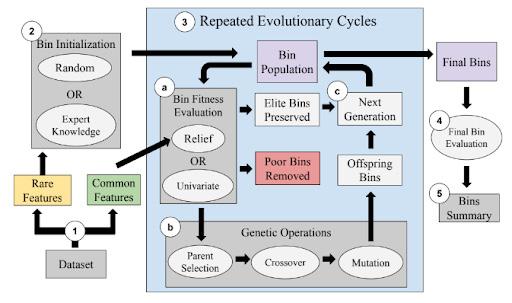
RARE is an EA that constructs bins i.e., candidate groups of features with rare states, seeking to optimize the relevant bin association with outcome. Figure 1 describes the main steps and components of the RARE algorithm including: (1) preprocessing, (2) bin initialization, (3) evolutionary cycles involving bin fitness evaluation and genetic operators, (4) final bin evaluation, and (5)
outputs and bin summary. RARE was designed to identify one or more candidate RVBs from the evolving bin population. To simplify analyses in this study we focus on the top performing bin identified, however RARE can also be applied to identify a set of candidate bins as engineered features for further analysis.
Preprocessing
After loading the target dataset, RARE begins by separating rare from common variant features. Rare state features will later be considered for inclusion in bins, while common state features are only utilized when evaluating bins for potential epistatic interactions. To separate rare variant from common variant features, RARE first calculates the MAF of each feature. In GWAS data, features are single nucleotide polymorphisms (SNPs) encoded as (0,1,2) corresponding to (AA, Aa, aa) genotype states. This study focuses on features encoded as SNPs, however many other variable types and encodings are possible. Assuming this SNP encoding, MAFs are calculated as the sum of feature values divided by twice the number of instances, i.e., the frequency of the ‘a’ allele. Rare variant features and common features are subsequently separated based on a user-specified MAF cutoff, typically 0.05 in GWAS [16]. Any feature with an MAF = 0 (e.g., zero variance predictors) are removed because they offer no predictive ability [12]. For non-genetic or
and (5) summary of the top bins.
Figure 1. Schematic diagram of RARE algorithm including (1) data preprocessing, (2) bin initialization, (3) evolutionary cycles consisting of bin fitness evaluation, genetic operations, and creation of the next generation, (4) final bin evaluation,
non-SNP data, RARE assumes that MAF indicates each feature’s frequency of nonzero values relative to other states. Given this assumption, the same MAF calculation can be applied to other feature types and datasets.
Bin Initialization
RARE offers both random initialization and the capability to import expert knowledge (EK) derived bins as an evolutionary starting point. By default, random initialization generates bins with different sizes to promote diversity of discovery and avoid assumptions about optimal bin size. Initialization with a fixed bin size will be discussed later. Random initialization is carried out based on the number of rare features in the dataset (F) and the following user-specified parameters: the maximum number of bins in the population (B), the minimum number of features per bin (M), and the maximum number of bins that can contain each rare feature (Cmax), specified to promote bin diversity. First, RARE randomly selects a number Cn ₃ [1,Cmax], inclusive, for each of F rare features to select the number of bins containing each feature. Next, M features are assigned to each bin. Then the remaining rare features are randomly distributed to bins. Lastly, any feature duplicates are deleted from respective bins and replaced with randomly chosen replacement features.
As an alternative to random initialization, EK bins, i.e., predetermined rare variant bins that are believed or known to be informative, can be imported to form the initial bin population. Notably, regardless of the initialization method, each bin represents a candidate engineered feature. Thus, for downstream bin evaluation, each bin’s rare features’ values for an instance are summed to determine the engineered feature’s state for that instance. In this way, the population of candidate bins is transformed into a new dataset for the bin fitness evaluation phase.
Evolutionary Cycles
Following bin initialization, RARE commences a user-specified number of evolutionary cycles, (i.e., learning iterations), including bin fitness evaluation, genetic operations, and establishment of the next generation of candidate bins. A larger number of cycles generally improves EA performance, but typically, the number of cycles is selected based on time constraints and available computing resources [33].
Bin Fitness Evaluation
At the start of each evolutionary cycle, the fitness of each candidate bin in the population is evaluated. RARE presents two options for fitness evaluation: univariate scoring and Relief-based scoring.
RARE implements univariate fitness evaluation using the chi-square test, a popular filter-based feature selection method in machine learning [9, 25]. This is in line with how RVBs have been evaluated within existing binning methods. Here, the chi-square test statistic serves directly as bin fitness as a myopic quantifier of bin association with outcome.
Alternatively, RARE can evaluate bin fitness using the MultiSURF algorithm. MultiSURF was implemented within the ReBATE software, a scikit-learn compatible suite of Relief-based feature importance algorithms that are effective at detecting features involved with both univariate and epistatic associations [31, 32]. MultiSURF was previously demonstrated to be the most reliable and effective Relief-based algorithm to date [32]. During each cycle of RARE, MultiSURF is applied at the rule-population level, i.e., the candidate bin population is converted to a dataset of newly engineered features. MultiSURF thus evaluates a given bin in the context of all other bins as well as (optionally) any common variants available. This gives RARE the capability to evaluate bins for not only univariate associations but inter-bin or bin-common variant interactions associated with outcome. While MultiSURF is regarded as being a computationally efficient strategy to detect feature interactions, it scales quadratically with the number of training instances. This necessitates an option in RARE for bin fitness evaluation to take place with a subset of instances.
Genetic Operations
During each evolutionary cycle of RARE, genetic operations take place after bin fitness evaluation. A generation of candidate bins is replaced by the next generation in two ways: preservation of elite bins and creation of offspring bins.
Elitism is an established addition to the traditional genetic algorithm that preserves a proportion of the highest-scoring solutions of a generation for the next generation [27]. In RARE, the user specifies an elitism parameter, E ₃ [0, 1) where it is recommended that E ≤ 0.5, that dictates the proportion of high-scoring bins that
are preserved for the next evolutionary cycle. Both elite and non-elite bins are available for parent selection in the next step.
Based on the maximum bin population size (B) and the elitism parameter (E), a total of ₃B × (1 − E)₃ offspring bins must be created for the next generation. Offspring bins are discovered using the genetic operations of parent selection, mutation, and crossover. A total of ₃(B × (1 − E))/2₃ pairs of parent bins are chosen using tournament selection, a probabilistic approach where bins with high fitness are more likely to be chosen as parents, and bins with lower fitness still have an opportunity to serve as parents and potentially lead to new fit offspring bins [11].
Each parent bin pair undergoes crossover and mutation to create a corresponding pair of offspring bins. RARE utilizes uniform crossover, as illustrated in Figure 2, where each pair of parent bins is initially copied to create a pair of offspring bins. Then, each feature in each of the two paired offspring bins has a chance to swap between bins with a given user-specified probability. After crossover, a standard mutation operation [3] is applied to each offspring bin, such that each feature in the offspring bin has a user-specified probability of being removed and each feature outside the bin has a proportionate mutation probability of being added to the bin. Since uniform crossover and mutation place no limits on the resulting size of offspring bins, RARE prevents drastic changes in bin size by checking if an offspring bin is over 50% larger than its paired offspring case and redistributing features in such a case.
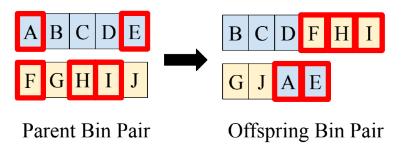
Figure 2. Illustration of RARE’s uniform crossover operation. Letters represent rare variant features. During crossover, features in each parent bin are chosen for crossover based on a user-specified crossover probability (these features are outlined in red in the figure). Features chosen for crossover in an offspring bin switch to its paired offspring bin.
Offspring bin pairs, created via parent selection, mutation, and crossover, are added to the elite bins to form the next generation. ‘Clean up’ operations are carried out on this new generation of bins to (1) delete any within bin feature duplicates (replacing any with a randomly selected alternative feature) and (2) delete any candidate bin duplicates (replacing any with a new randomly generated bin). Lastly, the new bins are engineered as features in an evaluation dataset to prepare for bin fitness evaluation at the start of the next evolutionary cycle.
Output and Bins Summary
After the user-specified number of evolutionary cycles are complete, RARE evaluates and outputs the final bins of rare variant features, along with the chi-square or MultiSURF value of each bin. RARE also presents a final engineered feature matrix, where each column represents a bin, to facilitate downstream machine learning. Further, a ‘top bins’ summary prints a list of features contained in each bin along with the the chi-square or MultiSURF value for each. The top bins summary also reports pertinent information related to each rare variant feature in the bins, such as the feature’s MAF and its original chisquare value, which is useful for assessing improved association post-binning.
RARE with Constant Bin Size
In certain problems, the user may know the bin size of the optimal bin solution or the user may want to find the optimal solution for bins of a certain size. Hence, we develop an alternate version of RARE with constant bin size, which differs from the standard version of RARE because (1) all bins are initialized with the same number of features, (2) bin size is held constant throughout the evolutionary cycles, and (3) RARE with constant bin size lacks the ability to discover optimal bin size during evolutionary cycles. To maintain a constant bin size throughout the evolutionary cycles, the uniform crossover operation is modified such that an equal number of features crossover from each offspring in the pair. The mutation operations is modified such that the number of features mutated inside the bin (i.e., features removed) is equal to the number of features mutated outside the bin (i.e., features added).
Experimental Evaluation of RARE
In order to conduct testing to evaluate RARE, we developed two Rare Variant Data Simulators (RVDSs): functions that create synthetic datasets to simulate different types of relationships in features with rare variant states based on user-specified parameters. RVDSs are applied to simulate datasets with underlying sets of rare variants that are maximally predictive when combined into an optimal bin. We simulate clean vs. noisy signal, as well as univariate vs. epistatic bin relationships.
Univariate Association Bin starts by randomly generating values (zero, one, or two) for each of the rare variant features that belong in the predictive bin. The bin value at each instance is calculated by summing the bin’s features’ values at each instance. Based on the user-specified cutoff metric, either mean or median of bin value across instances, instances with a bin value below the cutoff receive a class value of zero, while other instances receive a class value of one. The remainder of the features, random features that do not belong in the bin, are randomly generated. This process is illustrated in Figure 3. After all feature values are assigned, a user-specified endpoint variation
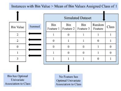
A univariate association RVDS was designed to generate a dataset containing rare variant features such that no single feature can independently predict class value, but a certain combination of features results in a fully penetrant bin, meaning the class label of an instance is completely dependent on the bin value at the instance. The user specifies the number of instances, the total number of rare variant features, the number of rare variant features that belong in the predictive bin, and the minor allele frequency cutoff defining a rare variant feature (e.g., 0.05). Based on these parameters, RVDS for
probability, a method of introducing noise, is applied to probabilistically switch the class value of each instance. RVDS for a Univariate Association Bin produces a feature matrix where a certain, user-known combination of rare variant features can be binned for optimal univariate association to class value.
RVDS for an Epistatic Interaction Bin
The second data simulator, RVDS for an Epistatic Interaction Bin, generates a dataset containing rare variant features and one common feature, such that
RVDS for a Univariate Association Bin
Figure 3. RVDS for a Univariate Association Bin
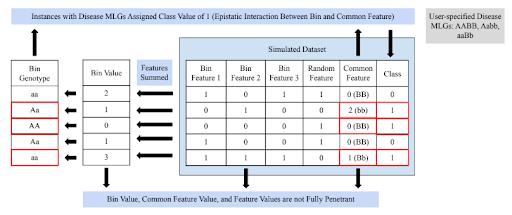
there exists an epistatic interaction between a bin of rare variant features and the common feature. This RVDS is inspired by the GAMETES software, which generates simulated SNP datasets with user-specified forms of epistatic interactions [30]. This RVDS starts by randomly generating values (zero, one, or two) for each of the rare variant features belonging in the epistatic interaction bin. Bin values at each instance are calculated by summing the bins’ feature’s values at the instance, and bin values of the instances are categorized into three groups to assign one of three bin ‘genotypes’ (AA, Aa, aa) to each instance. Similarly, a common feature value of zero, one, or two is assigned to each instance; a common feature value of zero corresponds to a BB common feature ‘genotype’, one corresponds to a Bb common feature genotype, and two corresponds to a bb common feature genotype. The user also selects which of the nine multilocus genotypes (MLGs) out of AABB, AABb, AAbb, AaBB, AaBb, Aabb, aaBB, aaBb, and aabb should correspond to disease status. For each of the instances whose bin value and common feature value matches an MLG of disease status, the class value will be one, while all other instances are assigned a class value of zero. Similar to the univariate RVDS above, random rare variant features, which do not belong in the bin, have their values randomly generated. The resulting dataset is generated in the form of a feature matrix where certain, user-known rare variant features can be additively grouped in a bin that holds an epistatic interaction with the common feature to predict class. The function also outputs the penetrance and frequency of each of the genotypes and MLGs, where penetrance is defined as an instance’s probability of having class value of one (i.e., disease status) [30]. A schematic of RVDS
for an Epistatic Interaction Bin is illustrated in Figure 4. This RVDS offers the user flexibility, as the user’s choice of which MLGs should correspond to disease status determines the type of relationship between the bin of rare variant features and the common feature. Certain combinations of disease status MLGs result in impure, strict epistatic relationships between the bin and common feature. On the other hand, other choices of disease status MLGs results in no bin value genotype and no common feature genotype being fully penetrant, which is an example of pure, strict epistasis.
Data Simulation Scenarios
Table 1 summarizes the various experimental simulation scenarios applied to test and evaluate RARE. Included is the experiment ID, RVDS association type (i.e., univariate or epistatic with a common variant), magnitude of noise, RARE initialization strategy used, fitness scoring used (i.e., Relief or univariate chi-square), total rare variants simulated in each dataset, the predictive rare variants simulated in each dataset, the MAF cutoff separating rare variant features from common variant features, and the number of instances in the simulated dataset. Experiments 1-4 examine RARE’s basic ability to identify RVBs from a randomly initialized population given different degrees of noise, specifically 0, 0.05, 0.1, and 0.5. Experiment 4 (noise = 0.5) has eliminated all associations and serves as our negative control. Experiment 5 (in comparison with 1) compares univariate association RVB detection performance using the more computationally efficient chi-square test fitness. Experiment 6 (in comparison with 1) examines the use of a constant bin size (assuming the optimal bin size is known). Here, the optimal bin size of 10 is applied. Experiment 7 (in
Figure 4. RVDS for an Epistatic Interaction Bin
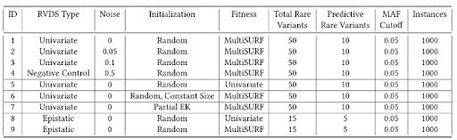
comparison with 1) examines how utilization of EK bins (when available) can improve efficiency of bin discovery. We simulate this here by initializing the bins such that they randomly include 50-80 % of the 10 predictive rare variants, and at least 4 non-predictive features. In Experiments 1-7, all simulated datasets contain 1000 instances, 50 total rare variant features, and 10 predictive rare variant features, that should be binned together for optimal univariate association with outcome.
Experiments 8 and 9 use the epistatic RVDS to create simulated datasets with 1000 instances, where 5 rare variant features, out of 15 total rare variant features, belong in a bin modeling a pure, strict epistatic interaction with a single common variable predictive of outcome. In the simulated datasets, AABB, AAbb, AaBb, aaBB, and aabb MLGs are denoted as having disease status and the common feature genotype frequency values are 0.25 for BB, 0.5 for Bb, and 0.25 for bb, such that all bin genotypes have a penetrance of 0.5 (i.e., bin values alone have no univariate association with outcome). Univariate fitness in Experiment 8 is compared to MultiSURF fitness in Experiment 9 to demonstrate the importance of the MultiSURF approach for detecting bin interactions.
Thirty replicates of each of the nine experiments are run (270 total trials). Univariate scoring is always carried out on all instances, while Relief-based scoring is done on a sub-sample of 500 out of the 1000 instances to reduce computational expense and evaluate efficacy of simple subsampling. RARE hyperparameter settings: maximum bin population size = 50, evolutionary cycles = 3000, elitism parameter = 0.4, crossover probability = 0.8, mutation probability = 0.1, are held constant throughout all experiments. Both population size and number of
evolutionary cycles are set modestly here to allow for evaluation of the 270 trials, but their increase would be expected to further improve performance in the future with a computational trade-off.
Results & Discussion
Here we summarize the results of applying RARE to the various RVDS datasets. All subsequent results are averages over 30 replicate trials for each experiment. For each scenario we highlight the average percent of ‘correct’ simulated predictive rare variants appearing in the ‘best’ bin identified by RARE. The ‘best’ bin is chosen based on the highest bin chi-square score for all univariate Experiments (1-7), regardless of the fitness metric used. Given that MultiSURF scores are calculated based on a sub-sample of instances, for epistatic Experiments (8-9) the ‘best’ bin was chosen as the one with the largest percentage of correct rare variant features, with percentage of incorrect features as a tiebreaker. We also report the percentage of incorrect rare variants from the data that were included. Note, these do not sum to 100 since we are examining bin composition with respect to features across the entire dataset. Further, for relevant experiments we report the optimal average chi-square scores obtained on respective RVDS datasets when all 10 user-known, correct rare variants (with no other variants) are included and evaluated as a bin. We contrast this with the average chi square scores of the best bin identified in each experiment with RARE. All p-values were < 0.001 from chi-square test in the 30 replicates for each of Experiments 1-3 and 5-7, while all p-values were > 0.05 from chi-square test in the 30 replicates for Experiment 4 (negative control). The chi-square degrees of freedom depended on the num-
Table 1: Experimental Data Simulation Scenarios for Evaluating RARE
ber of unique bin sums across all instances in the dataset. This is why large chi-square values were observed in these analyses.
Constructing Univariate Association Bins
were tested. Specifically, the adoption of the univariate chi-square value for RARE fitness (Experiment 5) yielded optimal RVB discovery across all 30 replicates. The lower performance observed in Experiment 1 is the result of only using half the training instances to reduce com-
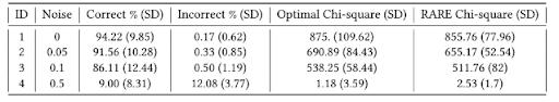
Table 2 presents average results, along with standard deviation (SD) of each metric across the 30 trials, for univariate bin association Experiments 1-4. Here, RARE applies random initialization and MultiSURF fitness. With a clean signal, Experiment 1 achieves high correct percentage and low incorrect percentage as well as a near optimal chi-square for the ‘best’ discovered bin. This is in direct contrast with Experiment 4 (negative control) where correct and incorrect rare variants were almost equally likely to have been included in the best discovered bin, which also yielded an expected low chi-square value. Note that in Experiment 4, the average ‘optimal bin’ chi-square value is lower than the average chi-square value of RARE’s best bin since class values are randomly assigned when noise = 0.5, so it is likely that a combination of randomly generated features have a higher univariate association to outcome than the bin of features that was optimal before noise was applied. Experiments 2 and 3 illustrate RARE’s ability to successfully manage a noisy association, despite expected reduced correct percentage and chi-square value, and increased incorrect percentage as noise increased in contrast with Experiment 1.
putational expense during MultiSURF fitness evaluation, rather than a reflection of MultiSURF’s ability to detect univariate associations. Next, utilizing a constant bin size (i.e., assumed optimum of 10) in Experiment 6 again improved performance over Experiment 1. This illustrates how precise or approximate knowledge of optimal bin size can be applied to improve RARE performance when available.
Table 4, offers a comparison of Experiment 1 to 7, i.e., random vs. EK bin initialization. We observe improved overall performance after all training cycles when adopting available EK bins to initialize the RARE population. Furthermore when we compare the number of evolutionary cycles RARE took to achieve an 80% solution, defined as a bin containing 80% of correct rare variant features and no more than 2 incorrect features, we found EK bin initialization to have dramatically improved RARE efficiency in bin discovery. This is consistent with the previous findings on improving EA efficiency by inputting partial EK [18]. The average run time for 3000 evolutionary cycles with Relief-based scoring in Experiments 1-4 and 6-7 was 24676.83 seconds and the average run time for univariate scoring in Experiment 5 was
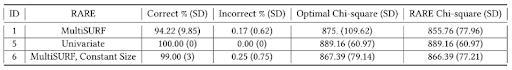
Table 3 offers a comparison of Experiment 1 to 5 and 6, where different configurations of the RARE algorithm
338.30 seconds. Clearly, univariate fitness is much more computationally efficient when searching for rare variant
Table 2: Univariate Association Bin Results with Noise
Table 3: Univariate Association Bin Results with Different RARE Configurations
bins of univariate effect. However in the next section we highlight the potential benefit of utilizing MultiSURF in RARE fitness for the detection of bin interactions.
Constructing Epistatic Interaction Bins
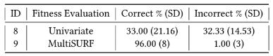
Table 5 presents the percentages of correct and incorrect features binned by RARE in the scenario involving a RVB having a pure interaction with a separate common variable (i.e. Experiments 8 and 9). As a strict, pure epistatic association, the optimal bin chi-square value is negligible (i.e. no univariate association). This was confirmed in experiment 9 which yielded an average top bin chi-square value of 0.68 (average p-value > 0.1). As one would expect, for experiment 8, univariate (chi-square) scoring failed to evolve bins that were informative in combination with the separate common variable since they do not consider multivariate interactions. This was evidenced by the similar inclusion of correct and incorrect rare variants in the best bins. Differently, RARE with MultiSURF (using all bins and the common variant to evaluate fitness), was successful in binning together correct rare variants and excluding incorrect ones. This illustrates the potential for RARE to be applied not only to detect RVBs with a univariate association, but also RVBs that are only informative in the context of other common variants and RVBs.
Conclusion
This study introduces the RARE algorithm, the first EA approach for engineering rare variant feature bins to improve power to detect both univariate or epistatic associations with outcomes. Over a variety of simulation studies, RARE reliably constructs (1) bins with optimal or near-optimal univariate association to outcome and
(2) optimal or near-optimal bins involved in an epistatic interaction with a common feature. While existing RVB tools can evaluate user-inputted bins of rare variants, RARE engineers bins from the ground up in a stochastic search for optimal bins. RARE can either discover novel bins from scratch when EK bins are not available or RARE offers the potential to improve upon existing EK bins that may be sub-optimal. This is because, unlike burden and non-burden tests used in genetics, RARE does not assume that solely rare variants belonging to the same genetic region should be grouped. In this work we have also presented two RVDSs that can be applied to generate a variety of rare variant simulation scenarios for testing or comparing other RVB methods in the future.
Conceived as a tool for rare variant association analysis, where there is significant uncertainty surrounding the role of rare variants, RARE can be applied to evolve bins of rare genetic variants to improve prediction of disease phenotypes and elucidate novel associations and interactions between rare variants, potentially contributing to the recognized missing heritability of complex diseases [24, 37]. Beyond genetics, RARE could also be applied to other biological data with rare variant states (e.g., HLA amino acid mismatches for predicting graft failure in organ transplantation) [5, 10, 34]. Similarly, RARE could be applied to a variety of data outside biology for binning features with rare feature states, such as near-zero variance predictors [12].
A limitation of this prototype RARE algorithm is the computational expense of MultiSURF-based bin evaluation since Relief-based algorithms scale quadratically with the number of instances. Such algorithms were designed to be run a single time on a given dataset rather than be run repeatedly once per evolutionary cycle, as is done in RARE. Thus, future investigations will explore (1) dual-scoring methods that integrate univariate scoring on the entire dataset and Relief-based scoring on a sample of instances and (2) parallelizable, intelligent instance sampling strategies for applying MultiSURF in RARE. We also plan to greatly expand simulation testing scenarios as well as real world biomedical applications with
Table 4: Univariate Association Bin Results with Random vs. Expert Knowledge Initialization
the aim of discovering predictive bins that reveal novel relationships among rare variants. Further, we expect to expand RARE by evaluating alternative implementation options and ultimately making it available as an open source scikit-learn Python package.
Acknowledgments
This work was supported by the following grant from the National Institute of Health: 1U01AI152960-01. Input from Dr. Loren Gragert of Tulane University School of Medicine and Dr. Malek Kamoun of Penn Medicine was very helpful throughout this work. Special thanks to Robert Zhang of University of Pennsylvania for his guidance and assistance in creating a GitHub repository for RARE. We also extend our gratitude to the Penn Medicine Academic Computing Services for use of their computing resources.
References
[1] Nadia Abd-Alsabour. 2014. A review on evolutionary feature selection. In 2014 European Modelling Symposium. IEEE, 20–26. https://doi.org/10.1109/EMS.2014.28
[2] Mattia Chiesa, Giada Maioli, Gualtiero I Colombo, and Luca Piacentini. 2020. GARS: Genetic Algorithm for the identification of a Robust Subset of features in high-dimensional datasets. BMC bioinformatics 21, 1 (2020), 54. https://doi.org/10.1186/s12859-020-3400-6
[3] Kalyanmoy Deb and Debayan Deb. 2014. Analysing mutation schemes for real-parameter genetic algorithms. International Journal of Artificial Intelligence and Soft Computing 4, 1 (2014), 1–28. https://doi.org/10.1504/ IJAISC.2014.059280
[4] James A Foster. 2001. Evolutionary computation. Nature Reviews Genetics 2, 6 (2001), 428–436. https://doi. org/10.1038/35076523
[5] Loren Gragert, Michael Halagan, and Martin Maiers. 2011. 32-OR: Clustering HLA alleles by sequence feature variant type (SFVT). Human Immunology 1, 72 (2011), S177.
[6] Tzung-Pei Hong, Chun-Hao Chen, and Feng-Shih Lin. 2015. Using group genetic algorithm to improve performance of attribute clustering. Applied Soft Computing 29 (2015), 371–378. https://doi.org/10.1016/j. asoc.2015.01.001
[7] Tzung-Pei Hong and Yan-Liang Liou. 2007. Attribute clustering in high dimensional feature spaces. In 2007 International Conference on Machine Learning and Cybernetics, Vol. 4. IEEE, 2286–2289. https://doi.org/10.1109/ ICMLC.2007.4370526
[8] Tzung-Pei Hong, Po-Cheng Wang, and Chuan-Kang Ting. 2010. An evolutionary attribute clustering and selection method based on feature similarity. In IEEE Congress on Evolutionary Computation. IEEE, 1–5. https:// doi.org/10.1109/CEC.2010.5585918
[9] Xin Jin, Anbang Xu, Rongfang Bie, and Ping Guo. 2006. Machine learning techniques and chi-square feature selection for cancer classification using SAGE gene expression profiles. In International Workshop on Data Mining for Biomedical Applications. Springer, 106–115. https://doi.org/10.1007/11691730_11
[10] Malek Kamoun, Keith P McCullough, Martin Maiers, Marcelo A Fernandez Vina, Hongzhe Li, Valerie Teal, Alan B Leichtman, and Robert M Merion. 2017. HLA amino acid polymorphisms and kidney allograft survival. Transplantation 101, 5 (2017), e170. https://doi. org/10.1097/TP.0000000000001670
[11] Padmavathi Kora and Priyanka Yadlapalli. 2017. Crossover operators in genetic algorithms: A review. International Journal of Computer Applications 162, 10 (2017).
[12] Max Kuhn et al. 2008. Building predictive models in R using the caret package. J Stat Softw 28, 5 (2008), 1–26. https://doi.org/10.18637/jss.v028.i05
[13] Seunggeung Lee, Gonçalo R Abecasis, Michael Boehnke, and Xihong Lin. 2014. Rare-variant association analysis: study designs and statistical tests. The American Journal of Human Genetics 95, 1 (2014), 5–23. https:// doi.org/10.1016/j.ajhg.2014.06.009
[14] Seunggeun Lee, Mary J Emond, Michael J Bamshad, Kathleen C Barnes, Mark J Rieder, Deborah A Nickerson, ESP Lung Project Team, David C Christiani, Mark M Wurfel, Xihong Lin, et al. 2012. Optimal unified approach for rare-variant association testing with application to small-sample case-control whole-exome sequencing studies. The American Journal of Human Genetics 91, 2 (2012), 224–237. https://doi.org/10.1016/j. ajhg.2012.06.007
[15] Bingshan Li and Suzanne M Leal. 2008. Methods for detecting associations with rare variants for common diseases: application to analysis of sequence data. The American Journal of Human Genetics 83, 3 (2008), 311–321. https://doi.org/10.1016/j.ajhg.2008.06.024
[16] Bingshan Li, Dajiang J Liu, and Suzanne M Leal. 2013. Identifying rare variants associated with complex traits via sequencing. Current protocols in human genetics 78, 1 (2013), 1–26. https://doi.org/10.1002/0471142905. hg0126s78
[17] Yulun Liu, Jing Huang, Ryan J Urbanowicz, Kun Chen, Elisabetta Manduchi, Casey S Greene, Jason H Moore, Paul Scheet, and Yong Chen. 2020. Embracing study heterogeneity for finding genetic interactions in large-scale research consortia. Genetic epidemiology 44, 1 (2020), 52–66. https://doi.org/10.1002/gepi.22262
[18] Qiang Lu, Jun Ren, and Zhiguang Wang. 2016. Using genetic programming with prior formula knowledge to solve symbolic regression problem. Computational intelligence and neuroscience 2016 (2016). https://doi. org/10.1155/2016/1021378
[19] Bo Eskerod Madsen and Sharon R Browning. 2009. A groupwise association test for rare mutations using a weighted sum statistic. PLoS Genet 5, 2 (2009), e1000384. https://doi.org/10.1371/journal.pgen.1000384
[20] Teri A Manolio, Francis S Collins, Nancy J Cox, David B Goldstein, Lucia A Hindorff, David J Hunter, Mark I McCarthy, Erin M Ramos, Lon R Cardon, Aravinda Chakravarti, et al. 2009. Finding the missing heritability of complex diseases. Nature 461, 7265 (2009), 747–753. https://doi.org/10.1038/nature08494
[21] Carrie B Moore, John R Wallace, Alex T Frase, Sarah A Pendergrass, and Marylyn D Ritchie. 2013. BioBin: a bioinformatics tool for automating the binning of rare variants using publicly available biological knowledge. BMC medical genomics 6, 2 (2013), 1–12. https://doi. org/10.1186/1755-8794-6-S2-S6
[22] Stephan Morgenthaler and William G Thilly. 2007. A strategy to discover genes that carry multi-allelic or mono-allelic risk for common diseases: a cohort allelic sums test (CAST). Mutation Research/Fundamental and Molecular Mechanisms of Mutagenesis 615, 1-2 (2007), 28–56. https://doi.org/10.1016/j.mrfmmm.2006.09.003
[23] Benjamin M Neale, Manuel A Rivas, Benjamin F Voight, David Altshuler, Bernie Devlin, Marju Orho-Melander, Sekar Kathiresan, Shaun M Purcell, Kathryn Roeder, and Mark J Daly. 2011. Testing for an unusual distribution of rare variants. PLoS Genet 7, 3 (2011), e1001322. https://doi.org/10.1371/journal.pgen.1001322
[24] Luisa F Pallares. 2019. Genetic Variation: Searching for solutions to the missing heritability problem. Elife 8 (2019), e53018. https://doi.org/10.7554/eLife.53018
[25] F. Pedregosa, G. Varoquaux, A. Gramfort, V. Michel, B. Thirion, O. Grisel, M. Blondel, P. Prettenhofer, R. Weiss, V. Dubourg, J. Vanderplas, A. Passos, D. Cournapeau, M. Brucher, M. Perrot, and E. Duchesnay. 2011. Scikit-learn: Machine Learning in Python. Journal of Machine Learning Research 12 (2011), 2825–2830.
[26] Jonathan K Pritchard. 2001. Are rare variants responsible for susceptibility to complex diseases? The American Journal of Human Genetics 69, 1 (2001), 124–137. https://doi.org/10.1086/321272
[27] Noraini Mohd Razali, John Geraghty, et al. 2011. Genetic algorithm performance with different selection strategies in solving TSP. In Proceedings of the world congress on engineering, Vol. 2. International Association of Engineers Hong Kong, 1–6.
[28] David E Reich and Eric S Lander. 2001. On the allelic spectrum of human disease. TRENDS in Genetics 17, 9 (2001), 502–510. https://doi.org/10.1016/S0168-
9525(01)02410-6
[29] Andrew N Sloss and Steven Gustafson. 2020. 2019 Evolutionary Algorithms Review. Genetic Programming Theory and Practice XVII (2020), 307–344. https://doi. org/10.1007/978-3-030-39958-0_16
[30] Ryan J Urbanowicz, Jeff Kiralis, Nicholas A Sinnott-Armstrong, Tamra Heberling, Jonathan M Fisher, and Jason H Moore. 2012. GAMETES: a fast, direct algorithm for generating pure, strict, epistatic models with random architectures. BioData mining 5, 1 (2012), 1–14. https://doi.org/10.1186/1756-0381-5-16
[31] Ryan J Urbanowicz, Melissa Meeker, William La Cava, Randal S Olson, and Jason H Moore. 2018. Relief-based feature selection: Introduction and review. Journal of biomedical informatics 85 (2018), 189–203. https://doi.org/10.1016/j.jbi.2018.07.014
[32] Ryan J Urbanowicz, Randal S Olson, Peter Schmitt, Melissa Meeker, and Jason H Moore. 2018. Benchmarking relief-based feature selection methods for bioinformatics data mining. Journal of biomedical informatics 85 (2018), 168–188. https://doi.org/10.1016/j.jbi.2018.07.015
[33] Pradnya A Vikhar. 2016. Evolutionary algorithms: A critical review and its future prospects. In 2016 International conference on global trends in signal processing, information computing and communication (ICGTSPICC). IEEE, 261–265. https://doi.org/10.1109/ ICGTSPICC.2016.7955308
[34] Adam Waring, Andrew Harper, Silvia Salatino, Christopher Kramer, Stefan Neubauer, Kate Thomson, Hugh Watkins, and Martin Farrall. 2020. Data-driven modelling of mutational hotspots and in silico predictors in hypertrophic cardiomyopathy. Journal of Medical Genetics (2020). https://doi.org/10.1136/jmedgenet-2020-106922
[35] Michael C Wu, Seunggeun Lee, Tianxi Cai, Yun Li, Michael Boehnke, and Xihong Lin. 2011. Rare-variant association testing for sequencing data with the sequence kernel association test. The American Journal of Human Genetics 89, 1 (2011), 82–93. https://doi.org/10.1016/j.
ajhg.2011.05.029
[36] Bing Xue, Mengjie Zhang, Will N Browne, and Xin Yao. 2015. A survey on evolutionary computation approaches to feature selection. IEEE Transactions on Evolutionary Computation 20, 4 (2015), 606–626. https://doi. org/10.1109/TEVC.2015.2504420
[37] Alexander I Young. 2019. Solving the missing heritability problem. PLoS genetics 15, 6 (2019), e1008222. https://doi.org/10.1371/journal.pgen.1008222
[38] Xinyuan Zhang, Anna O Basile, Sarah A Pendergrass, and Marylyn D Ritchie. 2019. Real world scenarios in rare variant association analysis: the impact of imbalance and sample size on the power in silico. BMC bioinformatics 20, 1 (2019), 1–10. https://doi.org/10.1186/ s12859-018-2591-6
[39] Or Zuk, Stephen F Schaffner, Kaitlin Samocha, Ron Do, Eliana Hechter, Sekar Kathiresan, Mark J Daly, Benjamin M Neale, Shamil R Sunyaev, and Eric S Lander. 2014. Searching for missing heritability: designing rare variant association studies. Proceedings of the National Academy of Sciences 111, 4 (2014), E455–E464. https:// doi.org/10.1073/pnas.1322563111
BreaNNa Barrett, alper caNBerk, cherIe FerNaNDes, & ethaN Markel
The following project is the work of the Hutchins Scholars ‘21 as they investigated a pond on campus during the summer of 2019. The work is part of the ecology portion of the program in which the Scholars investigated the pond’s water quality and biodiversity.
puriFying pond water through modular Filtration and chemical treatment
Breanna
Barrett1, Alper Canberk1, Cherie Fernandes1, & Ethan Markel1
1The Lawrenceville School
Abstract
According to the World Health Organization (WHO), 785 million people lack access to a source of drinking water, and contaminated drinking water is estimated to cause 485,000 deaths annually. This is a particular problem in developing countries, but the planet’s dwindling water supply has the potential to affect the world at large. It is thus becoming increasingly apparent that water scarcity is an issue that must be addressed on a global scale. Consequently, research into the development of sustainable methods of water purification has been particularly relevant in recent years. To address the issue, the members of the Lawrenceville Hutchins Class of 2021 created and tested a system that successfully purifies water from the Lawrenceville School pond within a $300 budget without any access to advanced lab technology. Within two weeks of research, mechanical design, and regular testing, an effective filter was built and proved consistent in successfully removing a host of harmful contaminants present in initial samples of pond water over the course of chemical treatment and modular filtration.
Introduction
The lack of safe drinking water is a global concern. In 2014, the city of Flint, Michigan, announced the detection of fecal coliform bacteria in its water source, which had been switched to Lake Huron via a new pipeline back in 2012 (“Flint Water Crisis Fast Facts”, 2019). In 2015, the Environmental Protection Agency (EPA) conducted an investigation on the city’s water in one of the resident’s homes and found 104 parts per billion (ppb) of lead, nearly seven times greater than the EPA limits of 15 ppb (CNN, 2019). To emphasize the importance of being able to attain potable water, this project simulated a hypothetical situation where the Lawrenceville campus loses the ability to pump its own water and is also unable to tap into the Lawrence Township water system, leaving the school pond as the only source of water. The assigned task was to purify the water so that the water satisfied the main areas of EPA-regulated standards for safe drinking water.
It was initially hypothesized that if the water in
the Lawrenceville School pond undergoes the following process—flocculation via the addition of alum; filtration through sand, gravel, activated charcoal, and cheesecloth; chlorination; addition of caustic acid, a base; and ion exchange via filtration through resin— then the pond will meet primary and secondary federal water standards as the combination of these processes will successfully remove contaminants and purify the water.
Challenges and Goals
Currently, data collection and observation indicated that nothing flows into the pond except rain water, making the water stagnant and preventing the flow of contaminants downstream. The possible contaminants found in pond water that are detrimental to human health are: feces, nitrates and nitrites, bacteria and heavy metals. In addition, the Pond water has a pH of 6, an acidity not within the federal standards.
Although there is not much water activity in the
pond, animals such as geese, fish, frogs and turtles that live in the pond are still active. Geese also deposit significant amounts of fecal matter into the pond. The feces not only form particles in the water that need to be filtered out of the water for human consumption but also release nitrates/nitrites and increase the concentration of fecal bacteria, Escheria Coli (E. coli), in the water. When present in large amounts, E.coli can cause gastrointestinal problems such as nausea, vomiting and diarrhea (Pietrangelo, 2019). If consumed by infants, water containing nitrates and nitrites can lead to methemoglobinemia, a blood disorder due to chemical alteration of hemoglobin structure by the nitrites and nitrates. When a hemoglobin turns into a methemoglobin due to the presence of nitrates/nitrites, respiratory systems in infants fail to deliver sufficient oxygen. Furthermore, “the strongest [pieces of] evidence for a relationship between drinking water nitrate ingestion and adverse health outcomes besides methemoglobinemia are colorectal cancer, thyroid disease, and neural tube defects” (Ward, et al., 2018).
When filtering pond water, the presence of heavy metals such as lead and copper is also taken into consideration. Lead poisoning causes a variety of symptoms ranging from high blood pressure to brain damage. According to the WHO, the Institute for Health Metrics and Evaluation (IHME) estimated that, in 2016, lead exposure accounted for 540,000 deaths. Due to toxicity of lead, even trace amounts of lead in the pond water has to be filtered. Additionally, the presence of copper also needs to be resolved. According to The New Hampshire Department of Environmental Services (NHDES), long term exposure to copper through drinking water can lead to anemia, kidney failure, and liver failure. Thus, copper had to be filtered out of the water as well to produce potable water.
The final problem was the pH of water. Although low pH does not make water dangerous to drink, it strongly reduces the aesthetic qualities of water. According to the EPA, water that has a pH below 6.5 tastes bitter and metallic. Since this experiment’s objectives included matching the EPA standards, the pH had to be raised. However, the side effects of raising the pH and treating the bacteria with chlorine raised the water’s hardness, creating another secondary aesthetic problem for the water that had to be solved.
Gridding of the Pond and Sampling Method
The pond was observed on three separate occasions during varying weather conditions, and it was found that each had different features which may affect the quality of the water. The features include the exposure to sun, wind current, depth of pond, and the presence of animals. The area was categorized and gridded as shown in Figure 1. Furthermore, there was a film of algae in the middle of the pond and oily substances on the surface of the pond near the road.
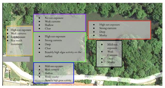
Each water sample was collected 30 cm below the surface, by dipping the test strips into the testing cups. No significant difference in water quality between regions was noted, and thus all pond water was subjected to the same purification treatment.
Initial Testing
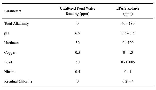
Table 1. Comparing initial pond water to EPA standards.
The chart above represents pond water taken from the black region on the map compared to the EPA standards for safe water. While the EPA has extensive criteria for potable water, only the high priority and primary standards as deemed by the EPA itself were investigated
Figure 1. Map of the School Pond Regions.
BreaNNa Barrett, alper caNBerk, cherIe FerNaNDes, & ethaN Markel
both in the initial pond water and the final product. The total alkalinity of the pond water tested well below the safe range. Related to the alkalinity is the pH, which was found to be at the bottom end of the safe range. However, hardness (referring to the traces of calcium and magnesium) and copper levels were within their respective EPA standards. Finally, the residual chlorine levels in the pond water were too low for potable water.
Treatment
Flocculation
Upon collection of pond water, flocculation was performed on the samples through the addition of alum powder (Al2(SO4)3) in the proportion 2.2 g per liter of water input. While alum powder is a cheap, relatively common household and culinary product (in keeping with the easily-accessible nature of all components of the filter), it is also a highly effective flocculant. Flocculants reduce the turbidity of water by aggregating colloids (suspended particles of sediment and debris), thus causing them to sink to the bottom of the container and separate from the liquid (“Flocculants and Coagulants”). It was found that the addition of alum in the aforementioned proportion, followed by a minute of stirring and eight minutes of wait time, greatly reduced the turbidity and odor of the pond water, effectively removing the majority of heavy metals and physical contaminants.
Chlorine Dioxide (ClO2)
Upon discovering that the pond water contains an unhealthy number of E. coli colonies, ClO2 tablets were used to eliminate the bacteria. When ClO2 is dissolved in water, it undergoes two chemical reactions:
ClO2 + e- –> ClO2 -
ClO2- + 4H+ + 4e- –> Cl- + 2H2O
In water, ClO2 gains an electron to produce a chlorite ion. Then, the chlorite ion attracts 4 hydrogen ions and gains four more electrons to produce water and a chlorine anion. The ability of ClO2 to gain many electrons allows it to directly react with and denature enzymes in bacteria. ClO2 was chosen instead of the conventional Cl2 because Cl2 can only gain 2 electrons as it reacts with water as opposed to ClO2, which can gain 5, making ClO2 around 2.6 times more effective at killing E. coli. In this experiment, 0.4 g Potable Aqua tablets were used to purify each liter of water. Once the tablets were dissolved, it took around
4 hours for the water to become completely disinfected.
Sand and Gravel
As a result of having a modular filter, there was an advantage of being able to alter the order in which the water would be purified. The sand and gravel removed the large debris from the pond water that was coagulated by the alum resulting in a lighter brown and less murky water. This filter was sealed at both ends with cheesecloth, that was porous enough to trap the smaller particles that the sand and gravel could not filter, but allowing the water to pass through.
Filtration through Activated Carbon/Charcoal
The water then went through the activated charcoal which removed nitrates, nitrites and certain heavy metals, which are all detrimental to human health. The filter was sealed with 2 sheets of filter paper in order to provide support to the system and remove the charcoal that was bonded to the water.
Ion Exchange
In order to moderate hardness, the water underwent the process of ion exchange, which was accomplished through filtration down a column of resin beads. Hard water is characterized by the presence of Ca2+ or Mg2+ ion deposits, and so ion exchange works to remove these ions in the process shown below (Fig. 2).
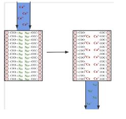
Figure 2. The process of ion exchange. Hard water (upper left) descends through a column of resin beads, each of which is covalently bonded to an anion group attached to a sodium ion (Na+), balancing the charges. Calcium has a higher metal reactivity than sodium, however, causing the two to exchange positions as the Ca2+ ions bump out the Na+ to join the compound in a single displacement reaction (Casiday and Frey).
pH Neutralization
Although the pH of the pond water (6.5) represented the bottom threshold of the pH safety range of the EPA, raising the pH so that it was well within the EPA safety range of 6.5 - 8.5 would be ideal. Furthermore, it was anticipated that the addition of chlorine and alum earlier in the filtration process would have extraneous effects on the pH. To address this imbalance in pH, sodium hydroxide solution (NaOH) was added to the water in the collection bottle at the bottom of the modular filter system. NaOH, a strong basic substance, is used by Lawrenceville’s own Brooks Well House to raise the pH of its water. Pure NaOH powder, however, was not directly added to the water, the final product. Instead, a solution of 0.5 M NaOH was created, which was then slowly added to individual 1 L increments of the 2 L of water that collected at the bottom of the modular filter.
Advantages of a Modular System
The main quality that makes this filtration system unique is modularity. The modular filter is composed of 5 parts: 2 L Bottle Reservoir at the top, sand/gravel module, activated charcoal module, resin module, and a water collecting bucket at the bottom. The parts screw onto each other with 3 inch male/female adapters, accelerating the process of assembly. Modularity gives this system 4 main advantages:
• Portability: The modular filter has high mobility. The parts can be disassembled and carried around.
• Ease of testing: Each part of the filter can be tested individually in order to figure out the effects of that particular module.
• Ease of manufacturing: Each module only consists of a PVC pipe, a male adapter, a female adapter, and arrangements of filtration materials (sand, gravel, charcoal, etc.) and filtration sheets (cheesecloth, coffee filter, filter paper). To construct a single module, an appropriate filtration material is first put into the PVC pipe, and then the filtration sheets are tightly held against the 2 openings of the pipe. To keep the filtration sheets in place, a male and a female PVC adapter are hammered onto the top and bottom of the column, respectively. Due to the simplicity of this process, many modules can be manufactured in a short amount of time.
• Ease of maintenance: Due to the fact that filtration materials and sheets can wear off, there has to be a way of replacing them. Compared to the conventional 1 piece filter that requires the entirety of the materials to be taken out in order for a single material in the middle to be replaced, replacing modular filter’s materials can be done with ease since individual parts of the filter can be disassembled without influencing other filtration materials.
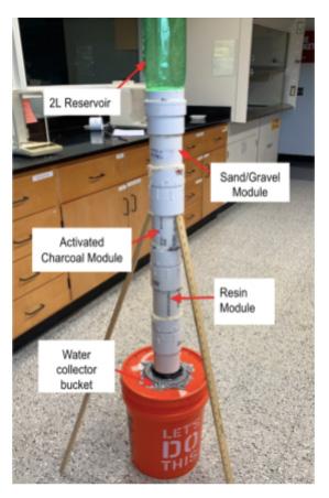
Figure 3. The structure of the water filter. The unfiltered pond water flowed in through 2.0 L reservoir and was passed through the sand/gravel module and into the activated charcoal module. The water then went through the resin module and the final product was collected in the water collector bucket.
Results and Analysis
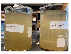
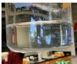
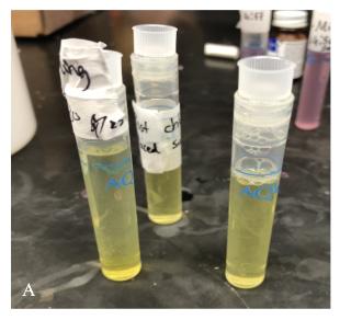
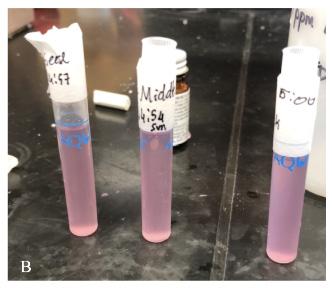
Figure 4. A visual comparison of the (A) unfiltered pond water with the (B) final filtered product.
Figure 5. A comparison of the (A) pond water pre-chlorine dioxide treatment with (B) water post chlorine dioxide treatment.
The images in Figure 5 are the coliform tests: the image with the red liquid is the test of pond water taken straight out of the pond with no treatment, and the image with the yellow liquid represents the water after being treated with 0.4 g of chlorine dioxide. Since chlorine is used by most public water systems as well as the Lawrenceville water purification system, it was considered as an ideal source for eliminating the microorganisms in the pond water. The results of the coliform test demonstrated that chlorine dioxide is effective in eliminating coliform from the pond water: the red liquid indicates a presence of coliform greater than 1 CFU/ml pre-treatment, while the yellow liquid post-treatment indicates that the coliform content was reduced to 0 CFU/ml.
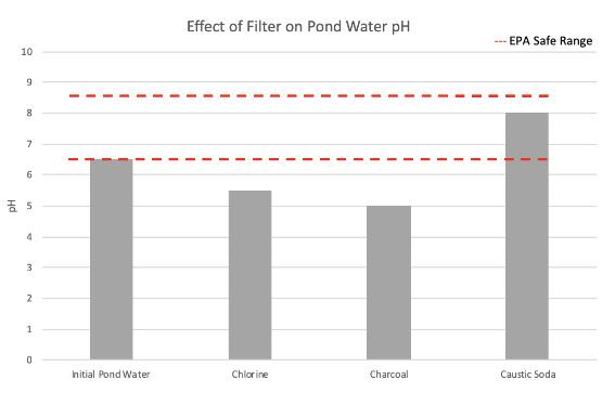
Initially when the pond water was sampled, it had a pH of 6.5, on the cusp of being in the safe range of the EPA standards. Then, after being treated with chlorine to remove bacteria, the pH lowered to 5.5 due to the acidic nature of the chlorine. Additionally, the pH was lowered to 5 by the charcoal due to the removal of the harsh metals, nitrates, and nitrites, all of which had alkaline qualities. The addition of the basic caustic soda made the pH of the now purified pond water safe and meet EPA standards.
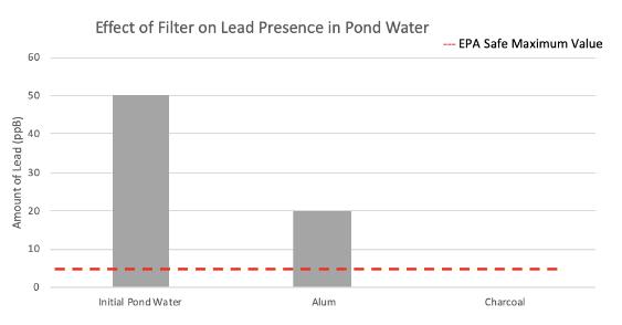
The amount of lead initially tested in 1 L of pond water (15 ppb) was well out of the EPA maximum safe level. This was surprising as it had been inferred that there would be little to no lead in the pond since lead is often only thought of as a concern as a leeching material into water flowing through metal pipes in most public water systems. Again, the modular design of the filtration system allowed for testing after each separate filter stage. After alum was added and given 4 hours to settle in the water, a testing strip revealed that lead had dropped to 20 ppb The ionic properties of alum (Al2(SO4)3), allow it to dissociate in water, and the ions that it forms bond to lead in the water, settling this debris to the bottom of the 1 liter beaker filled with pond water (Ackerman, 2018). No significant difference was noted in the lead levels after the sand and gravel filter module. However, a test of the water following activated charcoal filtration revealed that virtually all of the lead had been removed from the water. The activated charcoal, being a very porous substance, absorbs any remaining microscopic substances that were not filtered out by the larger gravel or sand particles, thus giving the activated charcoal the ability to remove lead.
Conclusion and Evaluation
It was hypothesized that the usage of a combination of modular filtration and chemical treatment would effectively purify pond water such that the resultant product would meet primary and secondary New Jersey drinking water standards. Post-analysis of the purified samples, it is evident that this hypothesis is valid; the water, initially rendered undrinkable by microorganism-related, physical, and chemical con-
Figure 6. The color scale of the coliform test, provided by the AquaVial Water Test Kit.
Figure 7. pH of water throughout the purification process.
Figure 8. The effect of the filtration process on the presence of lead (ppb) in pond water.
taminants, emerged from the filter purified and drinkable. Flocculation significantly reduced the turbidity of the water and separated physical contaminants, notably reducing lead content. Chlorine treatment eliminated all coliforms and potentially pathogenic bacteria. Sand and gravel filtration removed all remaining sediment and dead organic material, while activated charcoal filtration rid the water of any remaining heavy metals, nitrates, and nitrites. Ion exchange successfully addressed water hardness, having the water also meet secondary, primarily aesthetic standards and thus ensuring quality. Finally, treatment with caustic soda served to neutralize the pH of the water, resulting in perfectly drinkable, quality water output generated via a cost-effective system.
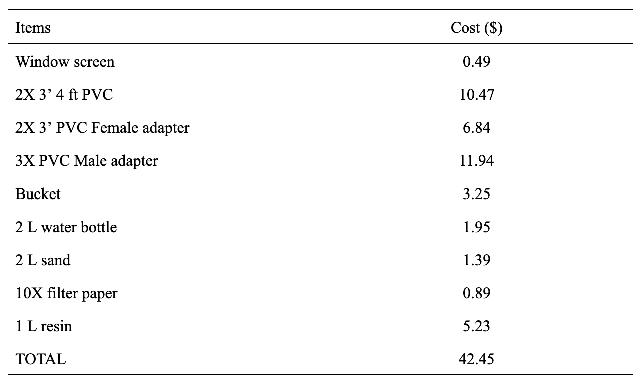
Acknowledgements
We thank Mr. Simpson, Dr. Fox, Mr. Ives, and Sahil Malhotra, who provided insight and expertise that greatly assisted this research. This research was supported by the 2020 Hutchins Summer Program.
References
Table 2. The cost of various items used to construct the filtration system.
The following project samples the work of Alexandra Pang ‘20 as she investigated the creation and expression of glycoproteins at the Robert Frederick Smith School of Chemical and Biomolecular Engineering in Cornell University. The work is part of the Delisa Research Group.
glycoSylation on a chip
Alexandra
Y. Pang1, Alicia K. Aquino2, Owen Haines-Burnham2, & Matthew P. DeLisa2
1The Lawrenceville School, NJ,
2Robert Frederick Smith School of Chemical and Biomolecular Engineering, Cornell University
Abstract
Glycans and glycoconjugates hold an important biological role in life, and bacterial cells can act as an optimal host for relevant proteins. One focus of the DeLisa Research Group is the “bottom-up” direct manufacturing of glycosylated proteins (“glycoproteins”) outside of the cell, with the aim of cost-effective production of useful therapeutic proteins. Previous projects from DLRG include the “Single Pot Glycoprotein Biosynthesis” which utilizes cell-free glycoprotein synthesis (CFGpS) (Thapakorn Jaroentomeechai, et al., 2018). For this project, the goal is to extract and engineer glycosylation enzymes (PglB, hGnTI, hGnTII, hGalT, hST6) from E. coli cells and conduct “glycosylation on a chip” in order to facilitate more efficient production of pharmaceutical proteins. Once proven to be successful with PglB and relevant enzymes, the microfluidic system will be implemented on alternatives such as yeast and human STT3s in the future.
Introduction
Glycans
Glycans are a generic term referring to any sugar or assembly of sugars, which are also commonly known as saccharides or carbohydrates (Bertozzi CR, et al., 2009). The biological roles of glycans vary in importance. Although there are glycans that appear to be insignificant, there are also others that are essential for the development, growth, functioning, or survival of the organism that synthesizes them (Varki A, Lowe JB, 2009).
Glycosylation
The glycosylation process is the enzyme-catalyzed covalent attachment of a carbohydrate to a polypeptide, lipid, polynucleotide, carbohydrate, or other organic compound. It is generally catalyzed by glycosyltransferases, and utilizes specific sugar nucleotide donor substrates. Glycosylation usually occurs naturally within living cells and there are two main glycosylation pathway sites:
N-glycosylation and O-glycosylation (Varki A, Sharon N, 2009).
Why Glycoprotein Engineering
By utilizing bacterial cells as hosts for proteins, new pathways can be synthetically engineered for the efficient production of biologically important glycans and glycoconjugates. In particular, Escherichia coli (E. coli) cells attached to the engineered proteins are able to act as a platform for the cost-effective biosynthesis of complex therapeutic proteins and development of human disease related vaccines (DeLisa Research Group, 2019).
Materials and Methods (Main Project – proof-of-concept with PglB)
PglB Engineering
PglB is a type of oligosaccharyltransferase complex (OST) that catalyzes the N-glycosylation of proteins. The scFV sequence was cut from the pspI01a-scFV-AviTag
plasmid through digestion to obtain the pspI01a-AviTag backbone. The PglB-10xHis insert was amplified by polymerase chain reaction (PCR) from PSN18-PglB-10xHis. The insert was ligated into the backbone, and the whole pspI01a-PglB-10xHis-AviTag plasmid was transformed into CLM24 cells and plated overnight.
Colony PCR was conducted on CLM24-pspI01aPglB-10xHis while the clones with PCR product were sequenced. Clone #3 was cultured in Lysogeny Broth (LB), grown overnight, and further subcultured in Terrific Broth (TB) until the measured absorbance (OD600) reached 0.5. Once the OD confirmed the sufficient amount of cell growth, CLM24-pspI01a-PglB-10xHis was induced overnight to extract the protein. After induction, PglB proteins were harvested through homogenization and ultra-centrifuging.
In addition to solubilized PglB proteins, the purified PglB with the polyhistidine-tag (His-tag) was also engineered into reusable beads, which offers an alternative in the chip attachment process.
Biotinylation
Biotin must be attached to the PglB protein for tethering onto the chip device. An overnight biotinylation reaction was set up with AviTagged PglB proteins. In order to check for biotinylation, a Western Blot was conducted on the PglB. The SDS-Page gel was run and transferred onto a membrane, which was blocked with BSA and incubated with extravidin (streptavidin).
Coomassie Blue Stain
The Coomassie Blue Stain stains all proteins present on the SDS-Page gel, which checks the purity of PglB proteins before glycosylation.
In Vitro Glycosylation (IVG) Reaction
IVG reactions are one of glycobiology’s most important extracellular glycosylation methods, which involves the glycosylation of a protein in a cell free environment.
IVG protocol for reference: Water, 10x IVG Buffer, 1M MnCl2, lipid-linked oligosaccharides (LLOs), sfGFP, PglB (purified PglB or PglB beads)
Anti-His and Anti-Glycan
Both Anti-His and Anti-Glycan antibodies confirm PglB’s ability to be glycosylated, using sfGFP in the IVG
reaction as an indicator. The sfGFP used in the IVG reaction was created using cell free protein synthesis (CFPS). The concentration of the sfGFP was measured using a Bradford Assay.
CFPS protocol for reference: Water, PJLI-sfGFP-DQNAT plasmid, RM (reaction mix), SS (salt), MM (master mix), T7 polymerase, lysate
For the Anti-His Western Blot, the membrane was first blocked with 5% milk before incubating with Anti-His antibodies. For the Anti-Glycan Western Blot, the membrane was blocked with BSA, incubated with Anti-Glycan antibodies, and further incubated with Anti-Rabbit antibodies. Between each incubation step, the membranes were washed with 10x TBST solution.
Sugar Manufacturing - Man3GlcNAc2
The ultimate goal of the device is to modify the Man3GlcNAc2 sugar. A starter culture of Man3GlcNAc2 was grown from freezer stock, which was subcultured in Super Broth (SB) , induced, and harvested after expression as LLOs. The Man3GlcNAc2 pellets were resuspended in methanol and vortexed before drying on glass plates overnight. CM (3:2 Chloroform Methanol) and CMW (10:10:3 Chloroform Methanol Water) were prepared and added to the LLOs. The LLOs were transferred into 50 mL conical flasks, then sonicated and centrifuged. Water was added and the process was repeated. Afterwards, methanol was added before the LLOs were spun down. The supernatant was transferred into a new conical before the addition of water and methanol to facilitate separation of the LLOs fractions. The fractions were spun down again and dried overnight on glass plates. After drying, the LLOs fractions were resuspended in the buffer.
Materials and Methods (Continuation of Main Project – Implementation
with hGnTI, hGnTII, hST6, hGalT)
The ultimate goal of the device is to modify the Man3GlcNAc2 sugar. A starter culture of Man3GlcNAc2 was grown from freezer stock, which was subcultured in Super Broth (SB) , induced, and harvested after expression as LLOs. The Man3GlcNAc2 pellets were resuspended in methanol and vortexed before drying on glass plates overnight. CM (3:2 Chloroform Methanol) and CMW (10:10:3 Chloroform Methanol Water) were pre-
pared and added to the LLOs. The LLOs were transferred into 50 mL conical flasks, then sonicated and centrifuged. Water was added and the process was repeated. Afterwards, methanol was added before the LLOs were spun down. The supernatant was transferred into a new conical before the addition of water and methanol to facilitate separation of the LLOs fractions. The fractions were spun down again and dried overnight on glass plates. After drying, the LLOs fractions were resuspended in the buffer.
Using the PET28a-AviTag-SIMPLEX-hGalT clones, hGalT was cut out from the plasmid with restriction enzymes. The PET28a-AviTag-SIMPLEX backbone was obtained through digestion. PCR was conducted on hGnTII and hST6, and the inserts were ligated respectively with the backbone after purification from the gel. The complete PET28a-AviTag-SIMPLEX-hGnTI and PET28a-AviTag-SIMPLEX-hST6 plasmids were sent to sequencing.
hGnTI, hGnTII, hGalT, and hST6 plasmids with the correct sequence were cloned and expressed in BL21(DE3) competent cells. The clones were further subcultured and induced before harvesting. A Coomassie Stain and a Streptavidin Western Blot were conducted on the clones to confirm their expression levels.
After their expression levels were confirmed, the hGnTI, hGnTII, hGalT, and hST6 plasmids were also transformed into SHuffle-pTRC-BirA competent cells and cloned for eventual use in the microfluidic device.
Results
PglB Engineering
The PCR product was clearly visible in clones #3 and #5 of CLM24-pspI01a-PglB-10xHis cells. Sequencing of aforementioned clones confirmed the attachment of AviTag onto the MBP.
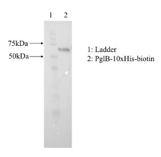
Figure 1. Western Blot of the Biotinylation reaction (2019). L1 contained the ladder. L2 contained the Pg1B-10xHis-biotin. The Western Blot results of the biotinylation reaction indicate the successful addition of biotin, which proves that the PglB can be biotinylated.
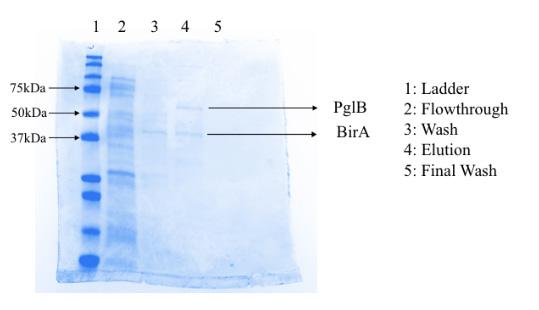
Figure 2. Coomassie Blue Stain (2019). The Coomassie Blue Stain with the clear band next to the ladder shows that PglB is pure.
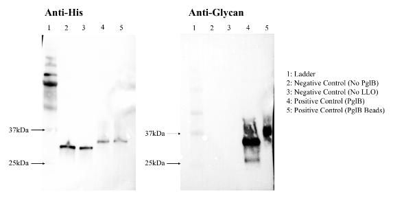
Figure 3. In Vitro Glycosylation (2019). The Western Blots of the Anti-His and Anti-Glycan antibodies show that sfGFP is glycosylated, which confirms that the PglB is active.
hGnTI, hGnTII, hST6, hGalT
Sequencing of PET28a-AviTag-SIMPLEX-hGalT clones and PET28a-AviTag-SIMPLEX-hGnTI clones confirmed that the plasmid was complete. Sequencing also confirmed the presence of AviTag within the PET28a-AviTag-SIMPLEX backbone and that hGnTII and hST6 were correctly inserted.
Conclusion and Future Direction
After demonstrating success with E. coli, the “Glycosylation on a Chip” microfluidic system can be tested and implemented on different proteins, particularly in human or mammalian cells of interest. Possible future alternatives include yeast and human STT3s.
Acknowledgements
Special thanks to Professor DeLisa for the research opportunity, and thank you to my mentor Alicia Aquino for all your guidance and support. Thanks to Owen Haines-Burnham and the rest of the DeLisa Research
Group for making this experience as enjoyable as it was.
DLRG Members:
Prof. Matthew DeLisa, Dr. Minji Li, Dr. Heng Li, Dr. Morgan Baltz Ludwicki, Dr. Aravind Natarajan, Dr. May Taw, Dr. Xiaolu Zheng, Dr. Emily Cox, Feng-Yang Chen, Ilkay Kocer, Thapakorn Jareontomeechai, Tyler Moeller, Kevin Weyant, Sean Chung, Alicia Aquino, Natalia Lopez-Barbosa, Weiyao Wang
Collaborators:
Zachary Manzer (Daniell Group, Cornell University), Prof. Alexander Frey (Aalto University), Jasmine Hershewe (Jewett Lab, Northwestern University)
References
Thapakorn Jaroentomeechai, et al. Single-pot glycoprotein biosynthesis using a cell-free transcri tion-translation system enriched with glycosylation machinery. Nature Communications, 9:2686, July 2018.
Bertozzi CR, et al., editors. Essentials of Glycobiology 2nd edition. Cold Spring Harbor (NY): Cold Spring Harbor Laboratory Press; 2009. Chapter 2. Rerieved from https://www.ncbi.nlm.nih.gov/books NBK1955/
DeLisa Research Group. Microbial Glycoengineering Retrieved from https://www.delisaresearchgroup.com/microb al-glycoengineering.
Varki A, Lowe JB. Biological Roles of Glycans. In Essen tials of Glycobiology. Chapter 6. Retrieved from https://www.ncbi.nlm.nih.gov/books/NBK1897/
Varki A, Sharon N. Historical Background and Overview. In Essentials of Glycobiology. Chapter 1. Retrieved from https://www.ncbi.nlm.nih.gov/books/ NBK1931/