Issuu

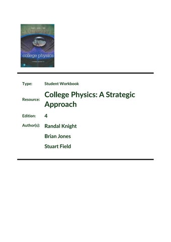
Type:

Student Workbook

Resource:

College Physics: A Strategic Approach

Edition:

Author(s):

Randal Knight Brian Jones Stuart Field

RANDALL D. KNIGHT

Knight | jones | field

“a P h 7] gy

‘

‘ é

a “VE

ayes a%

My)y's: Nid f 4, A.Cx ‘ w\\ 1

eM.

Py ag

“we Ny

)

\ Ny a)

wit

yy’

ele) iiclefomelayyscilers a strategic approach 4e

STUDENT

WORKBOOK

college physics >

hats esata approach 4e

knight - jones - field

randall d. knight California Polytechnic State University, San Luis Obispo

P, Pearson

Editor in Chief, Director Physical Science Courseware Portfolio: Jeanne Zalesky Courseware Portfolio Manager: Darien Estes Senior Content Producer: Martha Steele Managing Producer: Kristen Flathman Courseware Director, Content Development: Jennifer Hart Senior Analyst, Content Development, Science: Suzanne Olivier

Courseware Editorial Assistant: Kristen Stephens

Rich Media Content Producer: Dustin Hennessey Full-Service Vendor: Nesbitt Graphics/Cenveo Compositor: Nesbitt Graphics/Cenveo Art and Design Director: Mark Ong, Side By Side Studios Interior/Cover Designer: tani hasegawa Cover Printer: LSC Communications Printer: LSC Communications Manufacturing Buyer: Stacey J. Weinberger/LSC Communications Product Marketing Manager, Physical Sciences: Elizabeth Bell

States of America. This publication is protected by copyright, and permission should be obtained from the publisher prior to any prohibited reproduction, storage in a retrieval system, or transmission in any form or by any means, electronic, mechanical, photocopying, recording, or otherwise. For information regarding permissions, request forms

and the appropriate contacts within the Pearson Education Global Rights & Permissions department, please visit www.pearsoned.com/permissions/.

PEARSON, ALWAYS LEARNING and Mastering™ Physics are exclusive trademarks in the U.S. and/or other countries owned by Pearson Education, Inc. or its affiliates. Unless otherwise indicated herein, any third-party trademarks that may appear in this work are the property of their

respective owners and any references to third-party trademarks, logos or other trade dress are for demonstrative or descriptive purposes only. Such references are not intended to imply any sponsorship, endorsement, authorization, or promotion of Pearson’s products by the owners of such marks, or any relationship between the owner and Pearson Education, Inc. or its affiliates, authors, licensees or distributors.

@ Pearson

ISBN 10: 0-134-60989-1; ISBN 13: 978-0-134-60989-8

Vet

ply,

3 ‘lable of Contents aa

Force and Motion

Chapter 1 Chapter 2 Chapter 3 Chapter 4 Chapter 5 Chapter 6 Chapter 7 Chapter 8

Representing Motion...

Part| Chapter 9 Chapter 10 — Chapter 11

Part Ill

.. . s,s

2-1 3-1

Forces and Newton's Laws of Motion...............2++eeee8008

4-1

Applying Newton's Laws.....-.

2982910

[)

@0GHS, ..

Circular. Motion, Orbits, and,Gravity, 20) 200% 92 0iet..

ae Seem

se. 5-1

oo: 6-1

Rotational Motions) ean..0exaccinen Jed len ee

7-1

Equilibrium:and:Elasticity c!. antaere

eee

8-1

erate,

9-1

Energyand Wore: 622 S02 084, OF OOO V SE DS Ta eee USING ENGTOY at eee aie esouc ss ee eae enter

10-1 Taal

Conservation Laws Momenttimes

28%, Gog

aici Wah

geen

Properties of Matter

Part IV

Oscillations and Waves

Chapter 17 Chapter 18 Chapter 19

1-1

Motion in One Dimension. ..:...0....:.... 2 - .—<——eene

Thermal Properties of Matter...

Part V

«ee

Vectors and Motion inTwo Dimensions. ............-+..+ee++e80:%

Chapter 12 Chapter 13

Chapter 14 Chapter 15 Chapter 16

meres oes me

(°c... -.:,. « «5 ose

FIUNGS «ccs scccwacs “ees ok a eat pce store ow esse acs) Jk cen

12-1 13-1

OSCIHIALIONS co asp uc anscmnsuctiche dus+ Fuge Saeeeie meee ie er ear eee 14-1 Traveling. Waves and SOUNC oo. 5c pn arene gallte ee tle pees See a eee 15-1 Superposition and Standing Waves. ............ 200. e seve aes 16-1

Optics Wave Optics) 21%, 2o 8 Ne ee, ER ee ae ee ee 17-1 RaVOPticsMed, ASERC, 9D SEM LN tren erage el ee 3s eo vere me area 18-1 Optical IMStremnennts me oe te epee a ee ere es wr gas Kyle oes eae 19-1

iV TABLE

OF CONTENTS

Electricity and Magnetism 20-1

Chapter 20

OE ge ee .. Electric Fields and-Forces gs 4b erat.

Chapter 21 Chapter 22 Chapter 23 Chapter 24 Chapter 25 Chapter 26

21-1 EB BSP Electric Potentials 9.3. sf. Gio2R 6B Aad oe i Currentand Resistancem., ct, s:. sunt cee el cts = sok cog ieee eee aes 22-1 CCUCUIES Foy tee esp eee lik orciao GR eeee as 5 Photseine go ei pos MagneticFieldsand:Forces Vacnc. f5 own Peds an eye we eee Bee eo EMUpduction aad.iM Waves a. us. sls. 4 aye aus amet eins ee AC Electricity, . 00... 6. ee RA bet. « ee.

23-1 24-1 25-1 26-1

Modern Physics Chapter 27

Relativity ....2no2aemiG.owtnicotevM basewisey. ..-Biiqed2...

Chapter 28

Quantum PhysiesstiaM

36 ews. Lenciwell ide 2soiot. ..

Chapter 29

Atoms.and. Molecules.

cc....2wih (Diet

Chapter30

AeaieedR .. - 28-1

oeisiagaA... .eyekegem ... 29-1

= NuclearPhysics .......... 0.0000 cece ee eee aged... Dynamics Worksheets Momentum Worksheets Energy Worksheets

27-1

30-1

Pretace It is highly unlikely that one could learn to play the piano by only reading about it. Similarly, reading

physics from a textbook is not the same as doing physics. To develop your ability to do physics, your instructor will assign problems to be solved both for homework and on tests. Unfortunately, it is our experience that jumping right into problem solving after reading and hearing about physics often leads to poor “playing” techniques and an inability to solve problems for which the student has not already been shown the solution (which isn’t really “solving” a problem, is it?). Because improving your ability to solve physics problems is one of the major goals of your course, time spent developing techniques that will help you do this is well spent. Learning physics, as in learning any skill, requires regular practice of the basic techniques. That is what this Student Workbook is all about. The workbook consists of exercises that give you an opportunity to practice techniques and strengthen your understanding of concepts presented in the textbook and in class. These exercises are intended to be done on a daily basis, right after the topics have been discussed in class and are still fresh in your mind. Successful completion of the workbook exercises will prepare you to tackle the more quantitative end-of-chapter homework problems in the textbook. You will find that many of the exercises are qualitative rather than quantitative. They ask you to draw pictures, interpret graphs, use ratios, write short explanations, or provide other answers that do not involve calculations. A few math-skills exercises will ask you to explore the mathematical relationships and symbols used to quantify physics concepts but do not require a calculator. The purpose of all of these exercises is to help you develop the basic thinking tools you’ll later need for quantitative problem solving. It is highly recommended that you do these exercises before starting the end-of-chapter problems. One example from Chapter 4 illustrates the purpose of this Student Workbook. In that chapter, you will read about a technique called a “‘free-body diagram” that is helpful for solving problems involving forces. Sometimes, students mistakenly think that the diagrams are used by the instructor only for teaching purposes and may be abandoned once Newton’s laws are fully understood. On the contrary, professional physicists with decades of problem-solving experience still routinely use these diagrams to clarify the problem and set up the solution. Many of the other techniques practiced in the workbook, such as ray diagrams, graphing relationships, sketching field lines and equipotentials, etc., fall in the same category. They are used at all levels of physics, not just as a beginning exercise. And many of these techniques, such as analyzing graphs and exploring multiple representations of a situation, have important uses outside of physics. Time spent practicing these techniques will serve you well in other endeavors. You will find that the exercises in this workbook are keyed to specific sections of the textbook in order to let you practice the new ideas introduced in that section. You should keep the text beside you as you work and refer to it often. You will usually find Tactics Boxes, figures, or examples in the textbook that are directly relevant to the exercises. When asked to draw figures or diagrams, you should attempt to draw them so that they look much like the figures and diagrams in the textbook. Because the exercises go with specific sections in the text, you should answer them on the basis of information presented in just that section (and prior sections). You may have learned new ideas in Section 7 of a chapter, but you should not use those ideas when answering questions from Section 4. There will be ample opportunity in the Section 7 exercises to use that information there. You will need a few “tools” to complete the exercises. Many of the exercises will ask you to color code your answers by drawing some items in black, others in red, and perhaps yet others in blue. You

need to purchase a few colored pencils to do this. The authors highly recommend that you work in pencil,

Vi PREFACE

rather than ink, so that you can easily erase. Few are the individuals who make so few mistakes as to be

able to work in ink! In addition, you’ll find that a small, easily carried six-inch ruler will come in handy for

drawings and graphs. As you work your way through the textbook and this workbook, you will find that physics is a way of

thinking about how the world works and why things happen as they do. We will primarily be interested in

finding relationships, seeking explanations, and developing techniques to make use of these relationships, only secondarily in computing numerical answers. In many ways, the thinking tools developed in this workbook are what the course is all about. If you take the time to do these exercises regularly and to review the answers, in whatever form your instructor provides them, you will be well on your way to success in physics. To the instructor: The exercises in this workbook can be used in many ways. You can have students work on some of the exercises in class as part of an active-learning strategy. Or you can do the same in recitation sections or laboratories. This approach allows you to discuss the answers immediately, to answer student questions, and to improvise follow-up exercises when needed. Having the students work in small groups (two to four students) is highly recommended. Alternatively, the exercises can be assigned as homework. The pages are perforated for easy tear-out, and the page breaks are in logical places so that you can assign the sections of a chapter that you would likely cover in one day of class. Exercises should be assigned immediately after presenting the relevant information in class and should be due at the beginning of the next class. Collecting them at the beginning of class, and then going over two or three that are likely to cause difficulty, is an effective means of quickly reviewing major concepts from the previous class and launching a new discussion. If used as homework, it is essential for students to receive prompt feedback. Ideally, this would occur by having the exercises graded, with written comments, and returned at the next class meeting. Posting fairly detailed answers on a course website also works. Lack of prompt feedback can negate much of the value of these exercises. Placing similar qualitative/graphical questions on quizzes and exams, and telling students at the beginning of the term that you will do so, encourages students to take the exercises seriously and to check the answers. Student feedback from end-of-term questionnaires reveals three prevalent attitudes toward the workbook exercises:

i. They think it is an unreasonable amount of work. i. They agree that the assignments force them to keep up and not get behind. ili. They recognize, by the end of the term, that the workbook is a valuable learning tool.

However you choose to use these exercises, they will significantly strengthen your students’ conceptual understanding of physics. Following the workbook exercises are optional Dynamics Worksheets, Momentum Worksheets, and Energy Worksheets for use with end-of-chapter problems in Parts I and II of the textbook. Their use is recommended to help students acquire good problem-solving habits early in the course. If you wish your students to use these, have them make enough photocopies for use throughout the term. Answers to all workbook exercises are provided as pdf files and can be downloaded from the Instructor Resource Area in Mastering™ Physics as well as from the textbook’s Instructor Resource Center at www.pearson.com.

Acknowledgments: the workbook.

The author would like to thank Cenveo Publishing Services for their production of

‘a Representing Motion 1.1 Motion: A First Look Exercises 1-3: Draw a motion diagram for each motion described below. Six to eight images are appropriate for most motion diagrams.

1. A car accelerates forward from a stop sign. It eventually reaches a steady speed of 45 mph.

2. A heavy rock is dropped over the edge of a cliff. Draw the motion diagram from tHe instant the rock is.released until the instant it touches the ground.

3. A skier starts from rest at the top of a 30° snow-covered slope and steadily speeds up as she skies to the bottom. (Orient your diagram as seen from the side. Label the 30° angle.)

2019 © Education, Pearson Inc.

1-1

1-2

CHAPTER

1 - Representing Motion

1.2 Models and Modeling Exercises 4—5: Draw a motion diagram for each motion described below. ¢ Use the particle model to represent the object as a particle. e Show the object at six or eight positions. ¢ Number the positions in order, as shown in Figure 1.4 in the text. 4. Alicia is driving at a steady 30 mph when the light ahead turns red. She immediately slows and stops. Show her motion from a few seconds before the light changes until she stops. Draw a vertical dashed line across your motion diagram to show the instant the light changes.

| —$—

>_>

.— Sp

re ;

5. Bob is standing on the ground. He throws a ball upward at a 45° angle. The ball lands on a second-story balcony. Show the motion from the instant the ball leaves Bob’s hand until the instant it touches the balcony.

z /‘

Exercises 6-9: For each motion diagram, write a short description of the motion of an object that will match the diagram. Your descriptions should name specific objects and be phrased similarly to the descriptions of Exercises 1 to 5 above. Note the axis labels on Exercises 8 and 9. 6.

Stops ' @

®@

e0e

Ban

4a)

8. | Vertical i

Horizontal

rey

=| = S a

0@ Starts

9. | North

& ee

e©eee

E ee

. ®

: Motion

Starts

Representing Motion -

CHAPTER 1

1-3

1.3 Position and Time: Putting Numbers on Nature 10. Using the particle model, redraw each of the motion diagrams from Exercises 1 to 3 in the space

below. Add a coordinate axis to each drawing and label the initial and final positions. Draw an arrow on your diagram to represent the displacement from the beginning to the end of the motion.

11. In the picture below, Joe starts walking slowly but at constant speed from his house on Main Street to the bus stop 200 m down the street. When he is halfway there, he sees the bus and steadily speeds up until he reaches the bus stop. a. Draw a motion diagram in the street of the picture to represent Joe’s motion. b. Add a coordinate axis below the picture with Joe’s house as the origin. Label Joe’s initial

position at the start of his walk as x;, his position when he sees the bus as xy, and his final

position when he arrives at the bus stop as x3. Draw arrows above the motion diagram to represent Joe’s displacement from his initial position to his position when he first sees the bus and the displacement from where he sees the bus to the bus stop. Label these displacements Ax, and Ax», respectively.

c. Repeat part b in the space below but with the origin of the coordinate axis at the location

2 SAS CSE ie a hs

Pearson 2019 © Education, Inc.

d. Do the displacement arrows change when you change the location of the origin? |

1-4

CHAPTER

| - Representing Motion

1.4 Velocity

12. A moth flies a distance of 3 m in only one-third of a second. a. What does theratio 3/(1/3) tell you about the moth’s motion? Explain.

b. What does the ratio (1/3)/3 tell you about the moth’s motion?

c. How far would the moth fly in one-tenth of a second?

d. How long does the moth take to fly 4 m?

132A. If someone drives at 25 mph, is it necessary that he or she does so for an hour?

b. Is it necessary to have a cubic centimeter of gold to say that gold has a density of 19.3 g/cm?? Explain. 2019 Inc. Education, © Pearson

Representing Motion

- CHAPTER

1-5

1.5 A Sense of Scale: Significant Figures, Scientific Notation, and Units 14. How many significant figures does each of the following numbers have?

a. 6.21

e. 0.0621

i. 1.0621

b. 62.1

f. 0.620

jp621e% 10:

c. 6210

g. 0.62

k. 6.21 X 10°3

d. 6210.0

h. .62

i 6210?

15. Compute the following numbers, applying the significant figure standards adopted for this text. a. 33.3 X 25.4 =

e, 2:34 * 31321 =

b. 33.3 — 25.4 =

c. 33.3 + 45.1 =

333° =

dos3%45,1 =

hey3s4=

SAS ya

16. Express the following numbers and comptted results in scientific notation, paying attention to significant figures.:

ax 9,827 =

d. 32,014 x 47 =

b. 0.000000550 =

@:,0,059)-22,304 —

c. 3,200,000 =

f. 320 X 0.050 =

17. Convert the following to SI units. Work across the line and show all steps in the conversion. Use scientific notation and apply the proper use of significant figures. Note: Think carefully about g and h. Pictures may help.

a. 9.12 ws = 9.12 ws X b. 3.42 km = 3.42 km X c. 44cm/ms = 44 cm/ms X

d. 80 km/hr = 80 km/hrX e. 60 mph = 60 mph X 2019 © Education, Pearson Inc.

f. 8in = 8in X

@ 14in? = 14 in? x h. 250 cm? = 250 cm? X

1-6

CHAPTER

| - Representing Motion

18. Use Table 1.4 and your common sense to assess whether or not the following statements are reasonable. Explain. See Examples 1.4 and 1.5 for examples of the type of reasoning needed.

a. Joe is 180 cm tall.

b. I rode my bike to campus at a speed of 50 m/s.

c. A skier reaches the bottom of the hill skiing at a speed of 25 m/s.

d. I can throw a ball ata distance of 2 km.

e. I can throw a ball at a speed of 50 km/hr.

f. Joan’s newborn baby has a mass of 33 kg.

g. A hummingbird has a mass of 3.3 g.

ee Inc. Education, Pearson 2019 ©

Representing Motion

-CHAPTER1

1-7

1.6 Vectors and Motion: A First Look 19. For the following motion diagrams, draw an arrow to indicate the displacement vector between the initial and final positions. ae@

@ @3

e 4

Ci 5

@0 @1

5°

20. In each part of Exercise 19, is the object’s displacement equal to the distance the object travels? Explain.

21. Draw and label the vectonsum, A a: B1 AO}O) 8 OF

geet A

Exercises 22-26: Draw a motion diagram for each motion described below. ¢ Use the particle model. ¢ Show and label the velocity vectors.

22. Galileo drops a ball from the Leaning Tower of Pisa. Consider the ball’s motion from the moment it leaves his hand until a microsecond before it hits the ground. Your diagram should be vertical.

Pearson 2019 © Education, Inc.

1-8

cHAPTER

1 - Representing Motion

23. A rocket-powered car on a test track accelerates from rest to a high speed, then coasts at constant speed after running out of fuel. Draw a vertical dashed line across your diagram to indicate the point at which the car runs out of fuel.

24. A bowling ball being returned from the pin area to the bowler starts out rolling at a constant speed. It then goes up a ramp and exits onto a level section at very low speed. You’ll need 10 or 12 points to indicate the motion clearly.

25. A car is parked on a hill. The brakes fail, and the car rolls down the hill with an ever-increasing

speed. At the bottom of the hill, it runs into a thick hedge and gently comes to a halt.

26. Andy is standing on the street. Bob is standing on the second-floor balcony of their apartment about 30 ft back from the street. Andy throws a baseball to Bob. Consider the ball’s motion from the moment it leaves Andy’s hand until a microsecond before Bob catches it.

]

Inc. Education, Pearson 2019 ©

se Motion in One

Dimension 2.1 Describing Motion 1. The position-versus-time graph on the right shows the position of an object moving in a straight line for 12 seconds.

x (m) 40

30 20 10 ° 4

a. What is the position of the object at 2 s, 6s, and 10 s after the start of the motion? At 2s:

cam!

At 6s:

At 10s:

b. What is the object’s velocity during the first 4 s of motion?

c. What is the object’s velocity during the interval from t= 4s tot=6s?

d. What is the object’s velocity during the 4 s from t=6s tot=10s?

2019 © Pearson Inc. Education,

e. What is the object’s velocity during the final 2 s from t= 10s tot=12s?

SEs,

2-2

CHAPTER

2 - Motion in One Dimension

2. Sketch position-versus-time graphs for the following motions. Include a numerical scale on both axes with units that are reasonable for this motion. Some numerical information is given in the problems. For other quantities, make reasonable estimates. Note: A sketched graph is hand-drawn, rather than laid out with a ruler. Even so, a sketch must be neat, accurate, and include axis labels.

a. A student walks to the bus stop, waits for the bus, and then rides to campus. Assume that all

the motion is along a straight street.

b. A student walks slowly to the bus stop, realizes he forgot his paper that is due, and quickly walks home to get it.

c. The quarterback drops back 10 yards from the line of scrimmage, and then throws a pass 20 yards to a receiver, who catches it and sprints 20 yards to the goal. Draw your graph for the football. Think carefully about what the slopes of the lines should be. 3)

S| = S P=8 oS =| as] ea) | —

ron So a © =

Motion in One Dimension

CHAPTER 2

2-3

3. Interpret the following position-versus-time graphs by writing a very short “story” of what is happening. Be creative! Have characters and situations! Simply saying that “a car moves 100 m to the right” doesn’t qualify as a story. Your stories should make specific reference to information you obtain from the graphs, such as distances moved or time elapsed. a. Moving car x (mi)

t (min)

b. Sprinter x (m)

100

80 60 40

t (s) 1

c. Two football players x (yards)

100 60

Brutus

Fred

716

t (s)

. The figure shows a position-versus-time graph for the motion of objects A and B that are moving along the same axis.

4 2

a. At the instant t= 1 s, is the speed of A greater than, less than,

engl

selkdntohains cK

SYAEs

MEE

ORES,

r(s)

2-4

CHAPTER

- Motion in One Dimension

5. Draw both a position-versus-time graph and a velocity-versus-time graph for an object that is at rest at x= 1 m. =

6. The figure shows six frames from the motion diagram So

of two moving cars, A and B.

a. Draw both a position-versus-time graph and a velocity-versus-time graph. Show the motion of both cars on each graph. Label them A and B.

b. Do the two cars ever have the same position at one instant of time? If so, in which frame number (or numbers)?

Draw a vertical line through your graphs of part a to indicate this instant of time.

7. Below are four position-versus-time graphs. For each, draw the corresponding velocity-versustime graph directly below it. A vertical line drawn through both graphs should connect the velocity v, at time t with the position x at the same time t. There are no numbers, but your graphs should correctly indicate the relative speeds.

Vy.

ape

E Cc.

: t

S ©

Motion in One Dimension

CHAPTER2

8. Below are two velocity-versus-time graphs. For each: ¢ Draw the corresponding position-versus-time graph. ¢ Give a written description of the motion. Assume that the motion takes place along a horizontal line and that x; = 0.

0 Por

a. Is the object moving the slowest without being at rest?

b. Is the object moving the fastest?

c. Is the object at rest?

0—

9. The figure shows a position-versus-time graph for a moving object. At which lettered point or points

d. Does the object have a constant nonzero velocity?

e. Is the object- moving to the left?

0 am

2-5

2-6

CHAPTER

2 - Motion in One Dimension

2.2 Uniform Motion

10. Sketch position-versus-time graphs for the following motions. Include appropriate numerical scales along both axes. A small amount of computation may be necessary. a. A parachutist opens her parachute at an altitude of 1500 m. She then descends slowly to earth at a steady speed of 5 m/s. Start your graph as her parachute opens.

b. A rabbit hops to the right at a steady 1 m/s for 4 s. It then sees a coyote and instantly increases its speed to 3 m/s.

c. Quarterback Bill throws the ball to the right at a speed of 15 m/s. It is intercepted 45 m away by Carlos, who is running to the left at 7.5 m/s. Carlos carries the ball 60 m to score. Let x = 0 m be the point where Bill throws the ball. Draw the graph for the football.

11. The height of a building is proportional to the number of stories it has. If a 25-story building is 260 ft tall, what is the height of an 80-story building? Answer this using ratios, not by calculating the height per story.

Motion in One Dimension

CHAPTER2

2-7

2.3 Instantaneous Velocity 12. Below are two position-versus-time graphs. For each, draw the corresponding velocity-versustime graph directly below it. A vertical line drawn through both graphs should connect the velocity v, at time t with the position x at the same time t. There are no numbers, but your graphs should correctly indicate the relative speeds. a . 7 0

De t

oa 0

13. The figure shows six frames from the motion E é diagram of two moving cars, A and B.

A®

a. Draw both a position-versus-time graph and a velocity-versus-time graph. Show both cars on each graph. Label them A and B. x

b. Do the two cars ever have the same position at one instant of time? If so, in which frame number (or numbers)?

Draw a vertical line through your graphs of part a to indicate this instant of time. c. Do the two cars ever have the same velocity at one instant of time? If so, between which two frames?

2-8

CHAPTER

2 - Motion in One Dimension

14. For each of the following motions, draw ¢ A motion diagram and ¢ Both position and velocity graphs.

a. A car starts from rest, steadily speeds up to 40 mph in 15 s, moves-at a constant speed for 30 s, and then comes to a halt in 5 s.

Vy.

b. A pitcher throws a baseball with a speed of 40 m/s. One-half second later, the batter hits the ball back toward the pitcher, just missing him, with a speed of 60 m/s. The ball is caught 1 s after it is hit. From where you are sitting, the batter is to the right of the pitcher. Draw your motion diagram and graph for the horizontal motion of the ball.

15. Which of the position-versus-time graphs below goes with the velocity-versus-time graph shown at the right? Circle the part label of your choice.

—

bios

Coe

Motion in One Dimension

CHAPTER2

2-9

2.4 Acceleration 16. The four motion diagrams below show an initial point 0 and a final point 1. A pictorial

representation would define the five symbols: xo, x), Vo,, Vj,, and a, for horizontal motion and equivalent symbols with y for vertical motion. Determine whether each of these quantities is positive, negative, or zero. Give your answer by writing +, —, or 0 in the table below. A

0 Gl [ee

Starts

Stops eR

eee ee

ie ia

earn

citer eeaens imeem 4

eee

0 D

0 Starts

0 Has initial velocity

Xo OF Yo

Vox OF Voy |

OF Vjx

xj Ory, V4

a, OF ay

17. The three symbols x, v,, and a, have eight possible combinations of signs. For example, one combination is (x, v,, a,) = (+, —, +). a. List all eight combinations of signs for x, v,, ay.

6. 7

2-10

CHAPTER

2 - Motion in One Dimension

b. For each of the eight combinations of signs you identified in part a: ¢ Draw a four-dot motion diagram of an object that has these signs for x, v,, and ay. e Draw the diagram above the axis whose number corresponds to part a.

¢ Use black and red for your ¥ and a vectors. Be sure to label thé vectors.

Motion in One Dimension

CHAPTER 2

2-11

2.5 Motion with Constant Acceleration 18. Draw a motion diagram to illustrate each of the following situations. a. ay =0 but v, ~ 0.

b. v, =0 but a, #0.

c. v= 0 and g, > 0.

19. The quantity y is proportional to the square of x, and y = 36 when x =3. id

UG ie te

b. Find x if y= 16.

c. By what factor must x increase for the value of y to double?

d. Consider the equation in your text relating Ax and At for motion with constant acceleration a,. Which of these three quantities plays the role of x in a quadratic relationship y = Ax*? Which plays the role of y?

20. Below are three velocity-versus-time graphs. For each, draw the corresponding accelerationversus-time graph. feu

me,

2-12

CHAPTER

2 - Motion in One Dimension

2.6 Solving One-Dimensional Motion Problems 21. Draw a pictorial representation of each situation described below. That is, (i) sketch the situation, showing appropriate points in the motion, (ii) establish a coordinate system on your sketch, and (iii) define appropriate symbols for the known and unknown quantities. Do not

solve. See textbook Example 2.10 as an example. a. A car traveling at 30 m/s screeches to a halt, leaving 55-m-long skid marks. What was the car’s acceleration while braking?

b. A bicyclist starts from rest and accelerates at 4.0 m/s? for 3.0 s. The cyclist then travels for 20 s at a constant speed. How far does the cyclist travel?

c. You are driving your car at 12 m/s when a deer jumps in front of your car. What is the shortest stopping distance for your car if your reaction time is 0.80 s and your car brakes at 6.0 m/s2?

College Physics A strategic Approach 4 ED Knight, Jones, Field Student Workbook