Sample Read
Contents PAGE
Module-wise Marks Distribution
I-5
Module-wise Comparison with Study Material
I-7
MODULE 1 ARITHMETIC Chapter 1 RATIOS, VARIATIONS AND PROPORTIONS
3
Chapter 2
TIME VALUE OF MONEY AND ANNUITY - SIMPLE AND COMPOUND INTEREST24
Chapter 3
ARITHMETIC PROGRESSION AND GEOMETRIC PROGRESSION
37
Chapter 4
TIME AND DISTANCE
49
MODULE 2 ALGEBRA Chapter 1
SET THEORY, VENN DIAGRAM
55
Chapter 2
INDICES AND LOGARITHMS
64
Chapter 3
PERMUTATION AND COMBINATIONS
82
Chapter 4
QUADRATIC EQUATION
96
I-9
TAXMANN®
I-10
CONTENTS PAGE
MODULE 3 CALCULUS - APPLICATION IN BUSINESS Chapter 1
CONCEPT OF CALCULUS AND ITS APPLICATION IN BUSINESS
109
Chapter 2
REVENUE AND COST FUNCTION
113
Chapter 3
OPTIMIZATION TECHNIQUES
117
MODULE 4 STATISTICAL REPRESENTATION OF DATA Chapter 1
TAXMANN®
INTRODUCTION
121
Chapter 2
DIAGRAMMATIC REPRESENTATION OF DATA
126
Chapter 3
FREQUENCY DISTRIBUTION
130
Chapter 4
GRAPHICAL REPRESENTATION OF FREQUENCY DISTRIBUTION – HISTOGRAM, 139 FREQUENCY POLYGON CURVE, OGIVE, PIE-CHART
MODULE 5 MEASURES OF CENTRAL TENDENCY AND DISPERSION Chapter 1
MEAN, MEDIAN, MODE, MEAN DEVIATION
143
Chapter 2
RANGE, QUARTILES AND QUARTILE DEVIATION
171
Chapter 3
STANDARD DEVIATION
178
Chapter 4
CO-EFFICIENT OF VARIATION
189
Chapter 5
KARL PEARSON AND BOWLEY’S CO-EFFICIENT OF SKEWNESS
194
CONTENTS
I-11 PAGE
MODULE 6 CORRELATION AND REGRESSION Chapter 1
SCATTER DIAGRAM
203
Chapter 2
KARL PEARSON’S CO-EFFICIENT OF CORRELATION
206
Chapter 3
REGRESSION ANALYSIS
221
MODULE 7 PROBABILITY Chapter 1
CONCEPTS AND TERMINOLOGIES
243
PRIMARY APPLICATIONS OF PROBABILITY THEOREMS
257
MODULE 8 INDEX NUMBER AND TIME SERIES Chapter 1
USES OF INDEX NUMBERS, METHODS OF CONSTRUCTION OF INDEX NUMBER
269
Chapter 2
COMPONENTS OF TIME SERIES AND CALCULATION OF TREND BY MOVING AVERAGE METHOD
281
Solved Paper : December 2024 (Suggested Answers)
P.1
Solved Paper : June 2025 (Suggested Answers)
P.11
Solved Paper : December 2025 (Suggested Answers)
P.21
TAXMANN®
Chapter 2
1 CHAPTER
<40= <4380= <>34 <40= 34E80C8>=
QUICK REVISION OF THE CHAPTER IMPORTANT CONCEPTS Objectives of Averaging: There are two main objectives of the study of averages:
(ii) To facilitate comparison. By reducing the mass of data to one single figure, compare various sets of data. Comparison can be made either at a point of time or over a period of time. Characteristics of a Good Average: Since an average is a single value representing a group of values, it is desirable that such a value satisfies the following properties: (i) It should be easy to understand. Since statistical methods are designed to simplify complexity, it is desirable that an average be such that it can be readily understood; otherwise, its use is bound to be very limited. (ii) It should be simple to compute. Not only an average should be easy to understand but also it should be simple to compute so that it can be used widely. However, though ease of computation is desirable, it should not be sought at the expense of other advantages, i.e., if in the interest of greater accuracy, use of a more difficult average is desirable one should prefer that. (iii) It should be based on all the observations. The average should depend upon each and every observation so that if any of the observation is dropped average itself is altered. (iv) It should be rigidly defined. An average should be properly defined so that it has one and only one interpretation. It should preferably be defined by an algebraic formula so that if different people compute the average from the same figures they all get the same answer.
143
TAXMANN®
(i) To get one single value that describes the characteristic of the entire data. Measures of central value, can be looked into as condensing the mass of data to one single value which, enable us to get an idea of the entire data. Thus, one value can represent thousands, lakhs and even millions of values.
144
MODULE 5: MEASURES OF CENTRAL TENDENCY AND DISPERSION
(v) It should be capable of further algebraic treatment. We should prefer to have an average that could be used for further statistical computations. For example, if we are given separately the figures of average income and number of employees of two or more factories we should be able to compute the combined average. (vi) It should have sampling stability. We should prefer to get a value which has what the statisticians call ‘sampling stability’. This means that if we pick 10 different groups of college students, and compute the average of each group, we should expect to get approximately the same values. It does not mean, however, that there can be no difference in the value of different samples. There may be some difference but those averages in which this difference, technically called sampling fluctuation, is less are considered better than those in which this difference is more. (vii) It should not be unduly affected by the presence of extreme values. If one or two very small or very large observations unduly affect the average, i.e., either increase its value or reduce its value, the average cannot be really considered as typical representative of the entire set of data. In other words, extremes may distort the average and reduce its usefulness. ARITHMETIC MEAN: TAXMANN®
A.M is denoted by x Bar. It is a mathematical measurement. Properties of Arithmetic Mean: (i) The sum of the deviations of the terms from the Actual mean is always zero. (ii) The sum of the squared deviations of the items from arithmetic mean is minimum i.e. less than the sum of the squared deviations of the items from any other value. (iii) If we have arithmetic mean and the number of items of two or more than two groups, we can calculate the combined average of groups. (iv) If the terms of a series are increased, decreased, multiplied or divided by some constant, the mean will also be increased, decreased, multiplied or divided by the same constant. (v) The standard error of the arithmetic mean is less than that of any other measure of central tendency. Merits of A.M: (i) Different interpretation by different persons not possible as AM is rigidly defined (ii) Easy to understand (iii) It takes all values in consideration (iv) It lends itself easily to further mathematical treatment Demerits of A.M: (i) It cannot be determined by inspection nor can it be located graphically (ii) It is affected very much by extreme values. Average of 1, 2 & 3 is 2 but average of 1, 2, 33 is extremely affected by presence of 33 and the result is 12 (iii) It cannot be calculated if the distribution has open ended classes
CH. 1 : MEAN, MEDIAN, MODE, MEAN DEVIATION
145
GEOMETRIC MEAN (g): The geometric mean is obtained by multiplying the values of the items together and then taking it to its root corresponding to the number of items. The Geometric mean is relative value and is dependent on all items. The geometric mean is never larger than the arithmetic mean. It is rare that it may be equal to the arithmetic mean. The Geometric mean of the products of corresponding items is two series is equal to product of their geometric means. Merits of G.M: (i) Different interpretation by different persons not possible as GM is rigidly defined. (ii) It takes all value in consideration. (iii) Unlike A.M, it is not affected much by the presence of extremely small or large values. (iv) It lends itself easily to further mathematical treatment. Demerits of G.M: (i) It is difficult to understand
(iii) It becomes imaginary if any of the observations is negative and GM is zero if any of the observation is zero HARMONIC MEAN: Harmonic mean is the reciprocal of the arithmetic mean Merits of H.M: (i) Different interpretation by different persons not possible as HM is rigidly defined. (ii) It takes all value in consideration. (iii) It is most suitable average when it is desired to give greater weight to smaller observations and less weight to the larger ones. (iv) It lends itself easily to further mathematical treatment. Demerits of H.M: (i) It is difficult to understand. (ii) It is difficult to compute. (iii) It is only a summary figure and may not be the actual item in the series. Relationship among the different Averages: In any distribution where the original items differ in size, then either the values of A.M > G.M > H.M (or) H.M < G.M < A.M. In case all items are identical then A.M. = G.M = H.M
TAXMANN®
(ii) It is difficult to calculate particularly when the items are very large or when there is graphical data
146
MODULE 5: MEASURES OF CENTRAL TENDENCY AND DISPERSION
MEDIAN AND OTHER POSITIONAL MEASURES: Median is denoted by Md. It is a positional measurement. Median divides a series into two equal parts. i.e., the middle most item is called median. Median divides the distribution into two equal parts. Quartile: Divides the distribution into 4 equal parts Decile: Divides the distribution into 10 equal parts Percentile: Divides the distribution into 100 equal parts Merits of Median: (i) It is not at all affected by the items on the extremes. (ii) It can be computed for the distributions which have open ended classes. (iii) The value of the median can be located graphically. (iv) The median is centrally located. The absolute sum of the deviations of the individual values from the median is always the minimum. Demerits of Median:
TAXMANN®
(i) In case of an even number of observations, median cannot be determined exactly. (ii) It does not lend itself to algebraic treatment in a satisfactory manner. (iii) It is unsuitable if it is desired to give greater importance to large or small values. MODE: It is denoted by ‘Mo’. Mode may be defined as the value that occurs most frequently in a statistical distribution. Uses of various Averages: (a) Arithmetic Mean: Arithmetic mean is considered to be an ideal average. It is frequently used in all the aspects of life. It possesses many mathematical properties and due to this it is of immense utility in further statistical analysis. In economic analysis arithmetic mean is used extensively to calculate average production, average wage, average cost, per capita income, exports, imports, consumption, prices etc. When different items of a series have different relative importance, then weighted arithmetic mean is used. (b) Geometric Mean: Use of Geometric mean is important in a series having items of wide dispersion. It is used in the construction of Index Number. The averages of proportions, percentages and compound rates are computed by geometric mean. The growth of population is measured in it as population increases in geometric progression. (c) Harmonic Mean: Harmonic mean is applied in the problems where small items must get more relative importance than the large ones. It is useful in cases where time, speed, values given in quantities, rate and prices are involved. But in practice, it has little applicability.
CH. 1 : MEAN, MEDIAN, MODE, MEAN DEVIATION
147
(d) Median and Partition values: Median and partition values are positional measures of central tendency. These are mainly used in the qualitative cases like honesty, intelligence, ability etc. In the distributions which are positively skewed, median is a more suitable average. These are also suitable for the problems of distribution of income, wealth, investment etc. (e) Mode: Mode is also positional average. Its applicability to daily problems is increasing. Mode is used to calculate the ‘modal size of a collar’, modal size of shoes,’ or ‘modal size of readymade garments’ etc. It is also used in the sciences of Biology, Meteorology, Business and Industry. IMPORTANT FORMULAS Arithmetic Mean 1. Discrete Data: (i) Direct Method: X = ∑ x /n (ii) Indirect Method: X = A + ∑ dx / n
X = A + ∑ dx i / n × i A = Assumed Mean dx = x – A dxi = (x – A)/i 2. Grouped Data: (i) Direct Method: X = ∑ fx / n (ii) Indirect Method X = A + ∑ fdx / ∑ f (iii) Step Deviation Method X = A + ∑ fdx i / ∑ f × i A = Assumed Mean dx = x – A dxi = (x – A)/i 3. Combined Mean: X = (n1 X1 + n2 X 2 ) / (n1 + n2 )
TAXMANN®
(iii) Step Deviation Method:
148
MODULE 5: MEASURES OF CENTRAL TENDENCY AND DISPERSION
4. Weighted Mean: Xlj = (w1 X1 + w2 X 2 )/(w1 + w2) Geometric Mean 1. Individual Series:
(
)
g = Antilog ⎡⎣ ∑ logx / n ⎤⎦ 2. Discrete Series:
(
)
g = Antilog ⎡⎣ ∑ fLogx / ∑ f ⎤⎦ 3. Continuous Series:
(
)
g = Antilog ⎡⎣ ∑ fLogm / ∑ f ⎤⎦ m = mid value of class interval 4. Weighted Mean:
(
)
g = Antilog ⎡⎣ ∑ wLogx / ∑ w ⎤⎦ TAXMANN®
5. Combined Mean: g = Antilog [(n1 log g1 + n2 log g2)/(n1 + n2)] Harmonic Mean 1. Ungrouped data:
(
H.M. = n / ∑ 1/ x
)
2. For data with Frequency:
(
H.M. = ∑ f / ∑ f / x
)
3. Weighted H.M.:
(
H.M. = ∑ w / ∑ w / x
)
Median: 1. Individual Series: M = (N+1)/2 th Observation 2. Discrete series with frequency: M = (N+1)/2 th Observation N = ∑f 3. Grouped Data (less than type): M = l + (N/2 – cf) × h/f l = lower boundary point of median class cf = cumulative frequency of previous class
CH. 1 : MEAN, MEDIAN, MODE, MEAN DEVIATION
149
f = frequency of median class h = width of the median class 4. Grouped Data (Greater than type): M = l + (N/2 – cf) x h/f l = upper boundary point of median class cf = cumulative frequency of succeeding class f = frequency of median class h = width of the median class Quartiles: Q1 = (N+1)/4 th Observation Q2 = M = 2 (N+1)/4 th Observation Q3 = 3 (N+1)/4 th Observation Deciles: D1 = (N+1)/10 th Observation D2 = 2 (N+1)/10 th Observation Other Deciles from D3 to D9 can be calculated similarly. P1 = (N+1)/100 th Observation P2 = 2 (N+1)/100 th Observation Other Percentiles from P3 to P99 can be calculated similarly. Note: Quartiles, Deciles and Percentiles for grouped data are calculated just like Median. Mode: 1. Individual Series: Value which occurs maximum times. 2. Discrete Series: Value with highest frequency. 3. Grouped Data: M0= l + (f0 – f1) × h/(2f0 – f1–f2) l = lower boundary point of modal class fo = Frequency of Modal Class f1 = Frequency of preceding class f2 = Frequency of succeeding class h = width of modal class Relation of Mean, Median and Mode: Mean – Mode = 3 (Mean – Median)
TAXMANN®
Percentiles:
150
MODULE 5: MEASURES OF CENTRAL TENDENCY AND DISPERSION
PAST EXAMINATION QUESTIONS THEORY QUESTIONS Q. 1. For a shoe-maker, which one of the following measures is most suitable to decide on the shoe sizes to manufacture?
Ans. (a) Uniformity in variability
(a) Median
Q. 6. Median is:
(b) Arithmetic mean
(a) Average point
(c) Mode
(b) Mid-point
TAXMANN®
(d) Geometric mean
[June 2013]
(c) Both (a) and (b) (d) None of these
[Dec. 2015]
(c) Most likely point
Ans. (c) Mode
(d) Most remote point [June 2016]
Q. 2. Rank of Kth decile is:
Ans. (b) Mid-point
(a) (n + 1)/2
Q. 7. Mode is the value which:
(b) (n + 1)/4
(a) Is a mid-point
(c) (n + 1)/10
(b) Occur the most likely
(d) k(n + 1)/10
[Dec. 2014]
(c) Average of all
Ans. (d) k (n + 1)/10
(d) Most remote
Q. 3. The third quarter is known as:
Ans. (b) Occur the most likely
(a) Lower quarter (b) Middle quarter
Q. 8. The middle most value of a frequency distribution table is known as:
(c) Upper quarter
(a) Mean
(d) None of these
[June 2015]
(b) Median
Ans. (c) Upper quarter
(c) Mode
Q. 4. ________ is known as positional average.
(d) Range
(a) Median
[June 2016]
Ans. (b) Median Q. 9. The first quarter is known as:
(b) Mean
(a) Lower quarter
(c) Mode (d) Range
[June 2016]
[Dec. 2015]
Ans. (a) Median Q. 5. The average discovers: (a) Uniformity in variability (b) Variability in uniformity of distribution
(b) Middle quarter (c) Upper quarter (d) None of these Ans. (a) Lower quarter
[June 2016]
151
CH. 1 : MEAN, MEDIAN, MODE, MEAN DEVIATION
Q. 10. ______ is the value of the observation having maximum frequency. (a) Mean
Q. 14. Empirical relation between mean, median and mode is expressed as Mean - Mode =
(b) Median
(a) 3 (Mean – Median)
(c) Mode
(b) 3 (Median – Mean)
(d) Standard Deviation [June 2017] [Modified]
(c) 3 (Mean – Mode)
Ans. (c) Mode Q. 11. The relation between A.M., G.M. and H.M. is expressed as:
(d) 3 (Mode – Mean) [June 2018] [Modified] Ans. (a) 3 (Mean – Median)
(b) A.M. < G.M. < H.M.
Q. 15. Harmonic mean of a set of observations is the reciprocal of the _______ of the reciprocal values of the observations.
(c) A.M. = G.M. = H.M.
(a) Mode
(d) Any of these [Dec. 2017] [Modified]
(b) Median
(a) A.M. > G.M. > H.M.
Ans. (a) A.M. > G.M. > H.M.
(d) Arithmetic Mean [June 2019] [Modified] Ans. (d) Arithmetic Mean
(b) Ten
Q. 16. The measure of central tendency of a statistical data which takes into account all the data
(c) Hundred
(a) Median
(d) Two [June 2018] [Modified] [Dec. 2019] [Modified]
(b) Mean
Ans. (d) Two
(d) Range
Q. 13. For a frequency distribution Median (Q2), 5th Decile (D5) and ____ Percentile have the same value.
Ans. (b) Mean
(a) Four
(c) Mode [Dec. 2019] [Dec. 2022]
(a) 25th
Q. 17. The cumulative frequency table is required to find out which of the following?
(b) 50th
(a) Mean
(c) 75th
(b) Median
(d) None of these [June 2018] [Modified] [Dec. 2019] [Modified]
(c) Mode
Ans. (b) 50th
(d) Range Ans. (b) Median
[June 2024]
TAXMANN®
Q. 12. Median is the value of a variable which divides the whole statistical data into ____ equal parts.
(c) Geometric Mean
152
MODULE 5: MEASURES OF CENTRAL TENDENCY AND DISPERSION
NUMERICAL QUESTIONS Q. 1. The algebraic sum of deviations of 10 observations from the constant C is –14 and the A.M. of the observations is 7.6. The value of C is:
Working Note:
(a) 8
10 = (x + y)/2
(b) 6
x + y = 20
(c) 9
x = 20 – y [Equation 1]
(d) 5
[June 2013]
A.M. = (x + y)/2
G.M. = (xy)1/2
Ans. (c) 9
6 = (xy)1/2
Working Note:
36 = xy [Equation 2]
Arithmetic Mean = C + ∑ d / n
Inserting Equation 1 in 2 We get,
7.6 = C + –14/10
(20 – y) y = 36 20y – y2 = 36
7.6 = C –1.4
y2 – 20y + 36 = 0
C=9 TAXMANN®
Let, the numbers be x and y
y2 – 18y – 2y + 36 = 0 Q. 2. If the H.M. of 4, x and 6 be 6, the value of x is: (a) 8
(y – 2) (y – 18) = 0 y–2=0
(b) 12
y=2
(c) 10 (d) 6
y (y – 18) – 2 (y – 18) = 0
[June 2013]
Ans. (b) 12 Working Note: H.M. = 3/(1/4 + 1/x + 1/6)
And y – 18 = 0 y = 18 So, the numbers are 2 and 18
5/12 + 1/x = 1/2
Q. 4. Heights (in cm) of 8 boys are: 70, 74, 70, 73, 72, 70, 74 and 70. The median is:
1/x = 1/2 – 5/12
(a) 70 cm
1/x = 1/12
(b) 71 cm
x = 12
(c) 72 cm
Q.3 A.M. and G.M. of two numbers are 10 and 6 respectively. The numbers are:
(d) None of the above [June 2013] Ans. (b) 71 cm
(a) 2 and 18
Working Note:
(b) 3 and 17 (c) 4 and 9
Arranging the values in ascending order we get, 70, 70, 70, 70, 72, 73, 74, 74
(d) None of the above [June 2013]
Median = (70 + 72)/2 = 71 cm
6 = 3/[(3 + 2)/12 + 1/x]
Ans. (a) 2 and 18
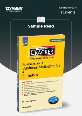
Fundamentals of Business Mathematics & Statistics (FBMS | Maths) | CRACKER AUTHOR : : PUBLISHER DATE OF PUBLICATION : : EDITION ISBN NO : : No. of Pages BINDING TYPE :
Tarun Agarwal Taxmann December 2025 4th Edition 9789375612858 328 Paperback
Rs. 395 DESCRIPTION Fundamentals of Business Mathematics & Statistics (FBMS | Maths) – CRACKER is an exam-focused practice book for CMA Foundation | Paper 3, fully aligned with the ICMAI syllabus and examination pattern applicable for the June/December 2026 exams. Adopting a problem-solving and MCQcentric approach, the book strengthens conceptual understanding while enhancing application skills in Business Mathematics and Statistics. It systematically analyses past examinations, converts descriptive questions into MCQs in line with current exam trends, and integrates chapter-wise summaries and practice questions to support effective revision and build scoring confidence. The Present Publication is the 4th Edition, authored by CA. Tarun Agarwal, with the following noteworthy features: •
[Aligned with the Latest ICMAI Syllabus] Complete adherence to the CMA Foundation Paper 3 curriculum for June/December 2026
•
[Past Examination Coverage up to December 2025] Fully solved MCQs based on previous CMA Foundation examinations
•
[Module-wise Marks Distribution Analysis] Insightful analysis of past exam weightage to identify high-scoring areas
•
[Study Material Mapping] Module-wise comparison with ICMAI Study Material for syllabus completeness
•
[Chapter-wise Tabular Summaries] Crisp tabular synopses at the beginning of each chapter for quick revision
•
[Extensive MCQ Practice] Coverage of 1050+ MCQs, including exam questions and practice problems
•
[Latest Exam Pattern Orientation] Descriptive past-exam questions converted into MCQs as per the current objective pattern
Buy Now