
Sample Read


© All rights reserved
Price : ` 325
Fifth Edition : June 2026
Published by :
Taxmann Publications (P.) Ltd.
Sales & Marketing : 59/32, New Rohtak Road, New Delhi-110 005 India
Phone : +91-11-45562222
Website : www.taxmann.com
E-mail : sales@taxmann.com
Regd. Office : 21/35, West Punjabi Bagh, New Delhi-110 026 India
Printed at :
Tan Prints (India) Pvt. Ltd.
44 Km. Mile Stone, National Highway, Rohtak Road Village Rohad, Distt. Jhajjar (Haryana) India
E-mail : sales@tanprints.com
Disclaimer
Every effort has been made to avoid errors or omissions in this publication. In spite of this, errors may creep in. Any mistake, error or discrepancy noted may be brought to our notice which shall be taken care of in the next edition. It is notified that neither the publisher nor the author or seller will be responsible for any damage or loss of action to any one, of any kind, in any manner, therefrom.
No part of this book may be reproduced or copied in any form or by any means [graphic, electronic or mechanical, including photocopying, recording, taping, or information retrieval systems] or reproduced on any disc, tape, perforated media or other information storage device, etc., without the written permission of the publishers. Breach of this condition is liable for legal action.
For binding mistake, misprints or for missing pages, etc., the publisher’s liability is limited to replacement within seven days of purchase by similar edition. All expenses in this connection are to be borne by the purchaser. All disputes are subject to Delhi jurisdiction only.


(c) A new and superior method of producing butter
(d) A decrease in the resources devoted to the production of investment goods. [Mar. 2016]
Q.4. Production possibility curves show maximum combinations of products.
(a)1
(b)2
(c)3
(d)4 [June 2016]
Q.5. Income minus Savings is equal to _________.
(a)Consumption
(b)Production
(c)Investment
(d)Demand [June 2017]
Q.6. ________ is an act to use the goods or service to satisfy the wants.
(a)Production
(b)Consumption
(c)Savings
(d)Distribution [Dec. 2017]
Q.7. The Production Possibility Curve (PPC) shows:
(a) The various combinations of two commodities is that can be produced by an economy
(b) The maximum production of goods
(c)Both (a) and (b)
(d)None of the above [Dec. 2022]
Q.8. The nature of the PPF curve is:
(a)Concave to the origin
(b)Convex to the origin
(c)Both (a) and (b)
(d)None of the above [June 2023]
Q.9. If an economy is working at the point to the left of the PPF curve, that indicates
(a)Excess production
(b)Unemployment
(c)Full employment
(d)None of the above [Dec. 2023]
ANSWERS:
CHAPTER 1.3
THEORY OF DEMAND, SUPPLY & EQUILIBRIUM DEMAND
Quick Revision of the chapter
Demand means desire backed by the purchasing power and willingness to pay the price. Demand is basically a purchase of any good or service which involves the expositions of the desire by the demander, the customer, and the ability of the demander. Ability or purchasing power is measured usually by the level of income and wealth of the customer.
DETERMINANTS OF DEMAND:
The demand for any commodity depends upon so many factors. These factors are called determinants of demand.
u Price of the goods: The demand for any commodity firstly depends upon its own price. When the price rises, demand decreases, and when the prices falls demand increases.
u Prices of the substitute goods: The demand for any commodity not only depends upon its own price but also the prices of its substitute goods. For example tea and coffee. Here the demand for tea depends upon price of the coffee.
u Prices of the complementary goods: The demand for a commodity also depends upon the price of its complementary goods. For example, car and petrol. Here the demand for petrol depends upon price of the car.
u Income of the consumer: The income of the consumer also influences the demand for a commodity. When the income rises, people purchase the more quantity of normal goods. When income falls they purchase less quantity of normal goods. But the reverse relation will work when the good will is inferior.
u Tastes and preferences of the consumer: The tastes and preferences of the consumer can also determine the demand for a commodity. When the tastes are changed, the demand for goods is also changed.
u Population: When the population size increases, the demand for goods also increases. When the population decreases demand also decreases.
u Climate: The climatic conditions also can influence the demand. In hot climatic conditions, cold drinks are demanded. In rainy season, the demand of umbrellas is increased.
LAW OF DEMAND:
The law of demand is a general statement stating that price and quantity demanded of a commodity are inversely related.
DEMAND FUNCTION:
Demand function explains the functional relationship between price and quantity demanded. According to the law of demand, when all other things remain constant (Ceteris Paribus), if the price of the good rises then its demand is decreased. If the price falls, demand will be increased. It means there is an inverse relationship between price and change in demand/change in price is negative in sign.
Dx = f [Px, Ps, Pc, Y, T]
Where, Dx = Demand for commodity X
F = Functional relationship
Px = Price of commodity
Ps = Price of substitute
Pc = Price of complementary good
Y = Income of consumer
T = Taste & preference of consumer
DEMAND SCHEDULE:
It shows the various quantities of the goods that are demanded at various levels of prices. There are two types of demand schedules:
Individual Demand Schedule: It shows the various quantities of a particular good that are demanded by an individual at various levels of prices in the market.
Market Demand Schedule: It shows the various quantities of the goods that are demanded by all the consumers (A, B, C, etc.) in the market at various levels of prices in the market. When the individual demands are added, market demand then is obtained.
CAUSES FOR FALLING NATURE OF DEMAND CURVE I.E. DOWNWARD SLOPING DEMAND CURVE:
u Law of diminishing marginal utility: According to law of diminishing marginal utility when the quantity of goods is more the marginal utility of the commodity will be less. So, the consumer demands more goods when the price is less. That is why, the demand curve slopes downwards from left to right.
u Substitution effect: In the case of substitutes, if the price of commodity ‘x’ rises relatively to the other good ‘y’ the consumer will buy less of commodity ‘x’ and buy more of the good ‘y’ which has become relatively cheaper. This is called substitution effect. So the demand curve slopes downward.
u Income effect: The income effect tells that the real income of the consumer rises due to the fall in the price level. So they purchase more and more goods when the price falls. This is said to be the income effect.
u New buyers: When the price of a commodity decreases, the new consumers are attracted to that commodity because when the price level falls it becomes cheaper good than before. So, the demand will rise when the price falls.
u Old buyers: When the price of anything decreases the old buyers purchase more goods than before. So the demand will be increased. That is why, the demand curve slopes downward from left to right.
EXCEPTIONS TO THE LAW OF DEMAND:
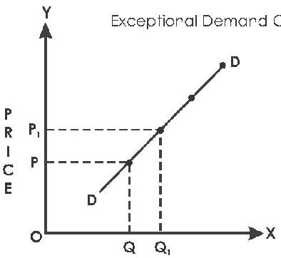
The law of demand is a general statement stating that price and quantity demanded of a commodity are inversely related. But in certain situations, more will be demanded at a higher price and less will be demanded at a lower price. In such cases, the demand curve slopes upward from left to right which is called an exceptional demand curve as shown in the following diagram.
Exceptional Demand Curve
When price increases from OP to OP1, quantity demanded also increases from OQ to OQ1. This is contrary to the Law of Demand.
u Giffen Paradox (Necessary goods): In the case of necessary goods, the law of demand cannot be operated. This is observed by British Economist, Sir Robert Giffen. He observed in London the low paid workers purchases more of bread when its price rises. That’s why, this situation is known as Giffen Paradox.
u Speculation: Some times the price of a commodity might be increasing and it is expected to increase further. The consumers will buy more of the commodity at the higher price than they did at the lower price. It is contrary to law of demand.
u Conspicuous: These are certain goods which are purchased to project the status and prestige of the consumer e.g., expensive cars, diamond jewellery, etc. Such goods will be purchased more at a higher price and less at a lower price.
u Shares or Speculative market: It is found that people buy shares of a company whose price is rising on the anticipation that the price will rise further. On the other hand, they buy fewer shares in case the prices are falling as they expect a further fall in price of such shares. Here, the law of demand fails to apply.
u Bandwagon effect: Here the consumer demand of a commodity is affected by the taste and preference of the social class to which he belongs to. If playing golf is fashionable among corporate executive, then the price of golf accessories rises, the business man may increase the demand for such goods to project his position in the society.
u Veblen Effect: Sometimes, consumers develop a false idea that high priced goods will have a better quality instead of a low priced good. If the price of such a good falls, they feel that its quality also deteriorates and they do not buy, which is contrary to the law of demand. It is also known as Veblen Effect.
3 TYPES OF DEMAND:
u Price demand: Price demand explains the relationship between price & demand for that commodity other things remaining constant. There is an inverse relationship between price and demand. So, the price demand curve slopes downwards from left to right. Dx = f (Px)
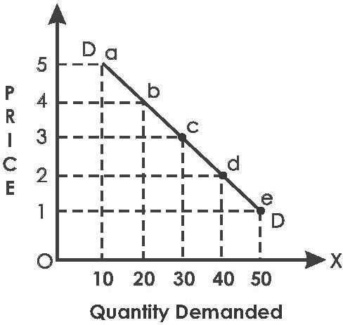
u Income demand: Income demand explains the functional relationship between income of consumer and demand for goods. Generally, if the level of income rises, the consumer purchases more goods. If the level of income decreases he purchases less quantity of goods. It means there is a direct proportional relationship between income of consumer and demand of goods. So, normally the income demand curve slopes upwards form left to right. Dx = f (y)
NORMAL/SUPERIOR GOODS
An increase in income leads to increase in demand & decrease in income leads to decrease in demand.
INFERIOR GOODS
An increase in income leads to decrease in demand.
Curve slopes upwards from left to right. Curve slopes upwards from right to left. Superior goods are equal to best quality goods. Inferior goods are equal to low quality goods.
Demand has direct relation with income.
Demand has indirect relation with income.
u Cross demand: It shows the relationship between price of one commodity and demand for another commodity. It means the demand for one commodity not only depends upon its price but also prices of its substitute goods and complementary goods. Dx = f (Py)
SUBSTITUTE GOODS
There is a direct proportional relationship between price of one commodity and demand for another commodity.
Example: Tea & coffee
If one good is used in the place of other good to satisfy the same want they are called substitute goods.
COMPLEMENT GOODS
There is an inverse relationship between price of one commodity and demand for another commodity.
Example: For construction we need cement, brick, etc.
If two ‘or’ more goods are used jointly to satisfy the single want they are called complementary goods.
The curve slopes upwards from left to right. The curve slopes downwards from left to right.
CHANGE IN DEMAND & CHANGE IN QUANTITY DEMANDED
CHANGE IN QUANTITY DEMANDED
Extension of demand
CHANGE IN DEMAND
Contraction of demand
Demand changes due to change in price. Demand changes due to change in other factors.
Other factors remain constant.
Changes occur on same curve.
Single curve is used.
If price decreases then the demand contracts moving the curve upwards.
If price increases then the demand extends moving the curve downwards.
Price remains constant.
Changes occur on different curves.
Different curves are used.
If other factors decreases then the demand contracts leading to shift of the curve towards left.
If other factors increases then the demand contracts leading to shift of the curve towards right.
3 TYPES OF ELASTICITY OF DEMAND
Elasticity means sensitiveness ‘or’ responsiveness. Elasticity of Demand means degree of response in demand. Due to different demand determining factors, the elasticity of demand explains the change in demand due to the change in the determinants of the demand.
u Price elasticity of demand: It shows the relationship between proportionate change in the demand and proportionate change in the price. It explains how much change in the price leads to how much change in the demand.
5 types of price elasticity of demand:
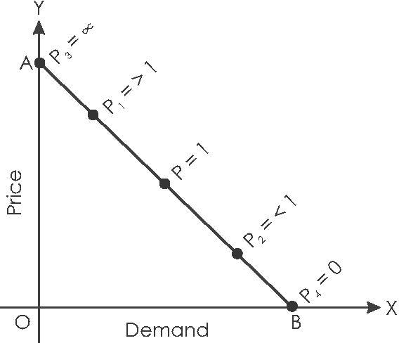
n Perfectly elastic demand (Ep = ∞)
n Relatively elastic demand (Ep > 1)
n Unitary elastic demand (Ep = 1)
n Relatively inelastic demand (Ep < 1)
n Perfectly inelastic demand (Ep = 0)
Ep = Proportionate Change in Demand
Proportionate Change in Price
u Income elasticity of demand: It shows the proportionate change in demand with respect to proportionate change in income. It means it explains how much change in the income leads to how much change in demand.
5 types of income elasticity of demand:
n Perfectly elastic demand (Ep = ∞)
n Relatively elastic demand (Ep > 1)
n Unitary elastic demand (Ep = 1)
n Relatively inelastic demand (Ep < 1)
n Perfectly inelastic demand (Ep = 0)
Ey = Proportionate Change in Demand
Proportionate Change in Income
u Cross elasticity of demand: It shows the proportionate change in demand for one commodity & proportionate change in price of another commodity. It means it explains how much change in the price of one commodity leads to how much change in demand of another commodity.
Ec = Proportionate Change in Demand of X
Proportionate Change in Price of Y
4 METHODS OF MEASUREMENT OF ELASTICITY OF DEMAND:
u Percentage Method: In this method, to measure the elasticity of demand firstly we should find out the change in demand and change in price in percentages.
u Total outlay method: In this method, on the basis of relationship between price and total expenditure elasticity can be decided
n If the total expenditure increases with the falling of the price and decrease with the raising of the price, it is said to be relatively elastic demand (EP > 1).
n With total expenditure remaining constant the increase ‘or’ decrease in price it is said to be unitary elastic (EP =1).
n If the total expenditure decreases with the falling of the price and increase with the raising of the price. It is said to be relatively in elastic demand (EP< 1).
Total Expenditure
u Point method: In this method the elasticity of demand can be measured at a particular point on the demand curve. In this method the following formula can be used:
u Arc method: If there are big changes in demand and prices it is not possible to measure the elasticity of demand by the point method. So, the Arc method is introduced.
IMPORTANCE OF ELASTICITY OF DEMAND
u Business Decision
u Monopolist
u Determination of factor price
u Route for international trade
u To the government
DETERMINANTS OF ELASTICITY OF DEMAND
u Nature of commodity
u Availability of substitutes
u Variety of uses
u Possibility of postponement of consumption
u Durable goods
THEORY OF CONSUMER BEHAVIOUR
Consumer surplus: The excess of price which a consumer would be willing to pay for a thing rather than go without the thing and over what he actually does pay.
Consumption: Consumption is defined as the satisfaction of human wants through the use of goods and services.
Concept of consumer surplus was introduced by Alfred Marshall. This concept is derived from the Law of Diminishing Marginal Utility.
Consumer Surplus ((C) S.) is the difference between willing price and actual price.
C.S. = Willing Price – Actual Price or
C.S. = Demand Price – Market Price
LAW OF DIMINISHING MARGINAL UTILITY
The law of D.M.U. was firstly propounded by H.H. Gosen in 1854. So, it is called Gosen’s first law of consumption. The law of D.M.U. was developed by Alfred Marshall. “The additional benefit which a person derives from a given increase in his stock of anything diminishes with every increase in the stock that he already has”. - Marshall
Total utility:
It is the total amount of satisfaction obtained by the consumer by the consumption of total units of a thing. The sum of marginal utilities is also called total utility.
TUx = f[Qx] Or TUx = ΣMUx
Marginal Utility:
It is the additional utility obtained by the consumer by the consumption of additional unit of a thing ‘or’ one more unit of a thing. The change in the total utility is also called marginal utility.
MUx = TUx – TUx – 1
Main Points:
u When total utility Increases, then the Marginal utility diminishes. So, T.U. Curve moves upward from left to right and M.U. curve slope downwards from left to right. However, this is only true when the law of diminishing marginal utility operates. Initially, it may so happen that the marginal utility might be rising along with the total utility curve for a particular commodity.
u When the total utility reaches the maximum, then the marginal utility is zero. At this point T.U. curve reached the peak stage and M.U. curve intercepts ‘X’ axis.
u When the total utility goes on diminishing then the M.U. becomes negative. So, the T.U. curves slopes downwards and M.U. curve crossed the x-axis.
Exceptions to Diminishing Marginal Utility:
u Collection of the rare goods
u Hobbies
u Misers
u Money and gold
u Reading of books
Demand Forecasting:
The success of the business firm depends upon the successful demand foresting. Estimation of future demand for product at present is called demand forecasting.
Methods of Demand forecasting:
u Expert opinion method
u Survey of buyers intentions
u Collective opinion method
u Controlled experiments
u Statistical method
SUPPLY
Supply means sum of the part of stock of the goods which is prepared by a seller to sell at a particular price, at a particular market in a particular period of time.
DETERMINANTS OF SUPPLY:
The supply of any commodity depends upon some factors. They are called determinants of the supply.
u Price of the goods
u Goals of the firm
u Inputs Prices
u Technology
u Government Policies
u Expectation about future prices
u Prices of the other commodities
u Number of firms in the market
u Natural factors
LAW OF SUPPLY
It explains the functional relationship between supply of a good and price of the good. When all other things remaining constant, if the price rises supply also increased, if the price falls supply also falls. It means there is direct or proportional relationship between price and supply.
SUPPLY FUNCTION:
The supply function explains the relationship between the supply and the factors that determines the supply. This can be explained through an equation:
Sx = f [Px, Pi, W, GP, T]
Where, Sx = Supply for commodity X
F = Functional relationship
Px = Price of commodity
Pi = Price of inputs
W = Weather
GP = Government policy
T = Technology
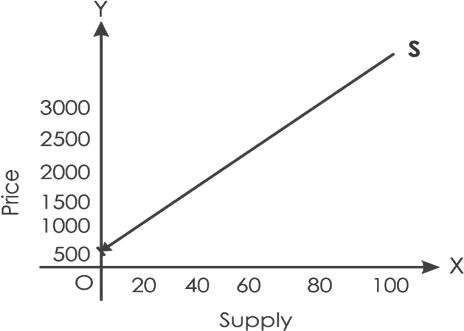
SUPPLY SCHEDULE:
It shows the various quantities of the goods that are supplied at various levels of prices.
u Individual supply schedule: It shows various quantities of the goods that are supplied by an individual seller (or) producer at various levels of prices in the market.
u Market Supply schedule: It shows the various quantities of the goods that are supplied by various producers (or) sellers at various levels of prices in the market. When we add the supply of all sellers then total supply ‘or’ market supply can be obtained.
EXCEPTIONS TO LAW OF SUPPLY
u Land
u Agricultural goods
u Rare goods
u Supply of labour
CHANGE IN QUANTITY
Extension of supply
SUPPLIED
CHANGE IN SUPPLY
Contraction of supply
Supply changes due to change in price. Supply changes due to change in other factors. Other factors remain constant.
Changes occur on same curve.
Single curve is used.
If price decreases then the supply contracts moving the curve upwards.
If price increases then the supply extends moving the curve downwards.
3 TYPES OF ELASTICITY OF SUPPLY
Price remains constant.
Changes occur on different curves.
Different curves are used.
If other factors decreases then the supply contracts leading to shift of the curve towards left.
If other factors increases then the supply contracts leading to shift of the curve towards right.
Elasticity means sensitiveness ‘or’ responsiveness. Elasticity of Supply means degree of response in supply. Due to different supply determining factors, the elasticity of supply explains the change in supply due to the change in the determinants of the supply.
u Price elasticity of supply: It shows the relationship between proportionate change in the supply and proportionate change in the price. It explains how much change in the price leads to how much change in the supply.
5 types of price elasticity of supply:
n Perfectly elastic supply (Es = ∞)
n Relatively elastic supply (Es > 1)
n Unitary elastic supply (Es = 1)
&
(FBEM | ECONOMICS) | CRACKER
AUTHOR : Leena Lalit Parakh
PUBLISHER : Taxmann
DATE OF PUBLICATION : June 2026
EDITION : 5th Edition
ISBN NO : 9789375617259
NO. OF PAGES : 248
BINDING TYPE : Paperback
DESCRIPTION
Fundamentals of Business Economics & Management (FBEM | Economics) | CRACKER is a dedicated practice companion for Paper 4 of the CMA Foundation examination conducted by The Institute of Cost Accountants of India (ICMAI). Rather than re-teaching the syllabus at textbook length, it distils each topic into a concise recap and then drills the student through a large, well-organised bank of objective questions—the format in which the Foundation paper is actually examined.
Following the signature teach-light, test-heavy approach of the CRACKER series, every chapter opens with a 'Quick Revision' of the key concepts (often as crisp comparison tables) and moves straight into MCQs drawn from past papers and current-pattern practice questions, each closing with an answer key. This lets a student summarise, drill, and self-check one topic at a time—ideal for the high-volume, objective nature of the exam.
This Edition is refreshed with fully solved questions and suggested answers up to the June 2026 examination, and is aligned with the latest ICMAI syllabus, the live MCQ pattern, and recent question trends—making it dependable for the December 2026 and June 2027 attempts.
The Present Publication is the 5th Edition | June 2026, authored by CA. Leena Lalit Parakh, with the following noteworthy features:
•[Fully Solved Past-Examination Questions Up To June 2026] Authentic questions from recent CMA Foundation papers with model/suggested answers, extended through the June 2026 sitting—so students practise on real examined material
•[950+ MCQs, including practice questions] Over 950 MCQs across all 21 chapters, blending genuine past-exam questions with practice questions, each chapter closing with a consolidated answer key
•[Descriptive Questions of Past Exams Converted into MCQs] Older descriptive and theory questions reframed into MCQ form to match the current objective pattern, preserving their value
•[A 'Quick Revision' Tabular Summary at the Start of Each Chapter] A concise, frequently tabular recap—for fast last-minute revision
•[Module-Wise Marks Distribution of Past Exams] A front-matter table mapping every chapter/topic to the marks it has carried (June 2023 to June 2026), with averages, showing exactly where marks cluster
•[Module-wise Comparison with the ICMAI Study Material] A mapping table aligning the book's five modules with the official ICMAI study-material modules, so nothing important is missed
•[Multiple Objective-Question Formats] Beyond standard four-option MCQs, True/False, fill-in-the-blanks, and statement/criterion-based questions, mirroring how ICMAI frames the paper