Stereo Miking: The Sound On Sound Guide 1st Edition

Includes comprehensive mics and accessories buyer’s guide PLUS detailed

Stereo Miking

The Sound On Sound Guide

A clear, practical guide to stereo recording in the real world!

LEARN HOW TO...

X Choose mics and recording techniques with confidence — for any source, in any space.

X Achieve stable, controllable stereo images without trial and error.

X Understand how stereo arrays really create width, depth and localisation.

X Record with both headphone and speaker playback in mind.

X Troubleshoot if things don’t go to plan.

Stereo

recording techniques

are the bread and butter of all serious recording engineers — and that isn’t about to change!

Introduction

Why Stereo?

HUGH ROBJOHNS

Despite today’s enthusiasm for multi-channel immersive audio formats such as Dolby Atmos, most people still listen in stereo, whether over speakers or on headphones. And even the mic techniques employed in immersive recordings are inherently based upon the trusted and proven principles and practices of stereo recording techniques, too. Obviously, then, understanding and mastering stereo recording techniques remains a core skill that everyone involved in recording and mixing audio must master.

In this guide, I’ll walk you through the fundamentals of how and why stereo recording and playback works — how our ears and brains manage to pinpoint where sound sources are located

around us — through the various ways in which we can convincingly mimic that positional information using speakers or headphones and a wide variety of stereo microphone arrays, to capture the optimum

SOS Technical Editor, Hugh Robjohns

understand how and why stereo recording actually works. I’ve included a number of illustrative audio examples, too, to help bring all those techniques and concepts to life. My aim is for the reader to

“Even the mic techniques employed in immersive recordings are inherently based upon the practices of stereo recording.”

blend of width, depth, detail and spaciousness. Perhaps I’ll be able to bust a few myths along the way too!

I’ve tried to write this guide in language that’s as accessible to recordists looking for practical advice as it is appealing to students and engineers who wish to better

emerge confident in how to choose appropriate recording techniques to deliver their desired result in any given situation, and how to adapt and optimise those techniques to overcome any practical difficulties encountered in real-world recording situations.

The Sound On Sound Guide

Stereo Miking

CONTENTS

Introduction By Sound On Sound’s Technical Editor, Hugh Robjohns.

6 Chapter 1: How We Hear In Stereo

To truly master stereo recording techniques, you must understand how your brain and your ears pinpoint the location of naturally occurring sounds.

12 Chapter 2: Emulating The Real World

The earliest attempts to convey a natural sense of sound positioning over speakers led to coincident mic techniques that remain popular today.

18 Chapter 3: Position & Perspectives

With careful placement and angling, coincident arrays can deliver a wide range of sonic perspectives.

26 Chapter 4: Mid-Sides Recording

The Mid-Sides technique employs a coincident array that’s unlike any other.

32 Chapter 5: Spaced Arrays

Spaced arrays offer a different set of pros and cons.

36 Chapter 6: Useful Software Tools

We introduce a range of tools that can help you set up and refine your stereo arrays with precision.

40 Chapter 7: Hybrid Stereo Arrays

If we wish to exploit the characteristics of spaced and coincident miking, we can use established arrays or even design our own.

44 Chapter 8: Advanced Hybrid & Combination Stereo Arrays

A deeper dive into hybrid arrays. What pitfalls might you encounter when using more than one array?

50 Chapter 9: Replicating Human Hearing

In this final chapter, we take inspiration from the human hearing system and explore the world of binaural recording, disc-shaped baffles and dummy heads.

58 Audio Demonstration Files

Chapters 1-9 refer to these audio demonstration files in detail, but here you’ll find an overview of the recording sessions, the mic setups, and where to find the files.

60 Stereo Miking Buyer’s Guide

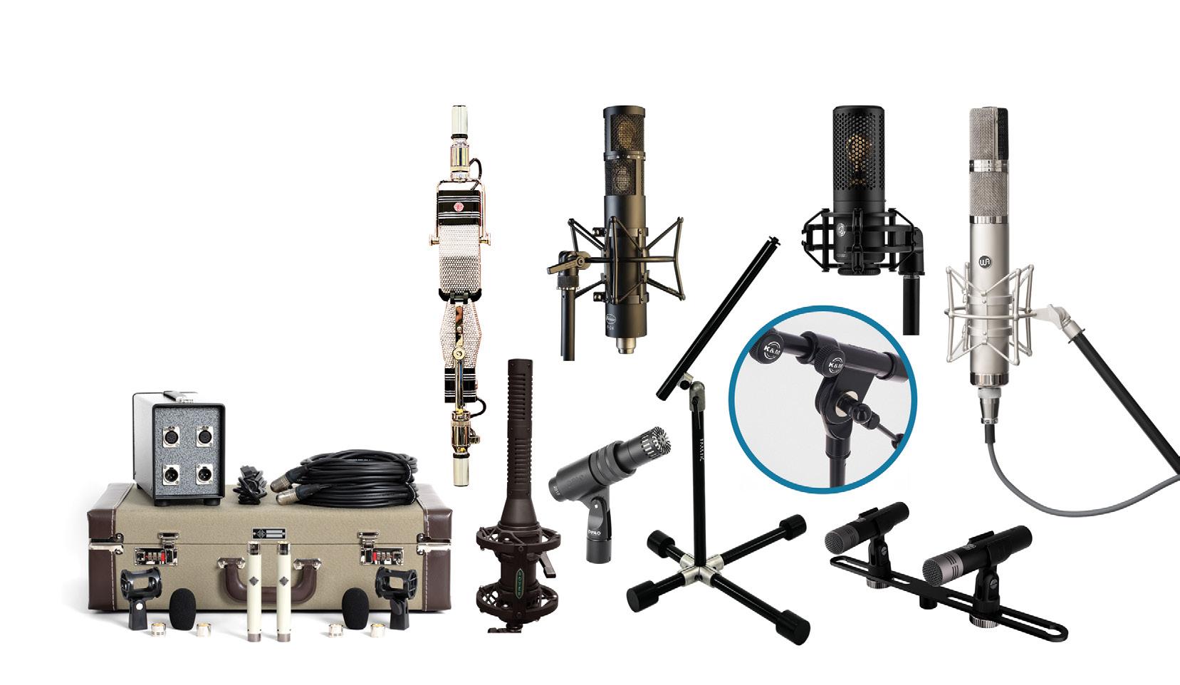
We shine a spotlight on the many reputable manufacturers who make stereo mics, closely matched individual mics, dedicated stereo sets, and related accessories.

72 Glossary

A full explanation of the technical terms, people and equipment discussed in this book.

Chapter 1

How We Hear In Stereo

To properly understand stereo miking, you need to start by exploring the most important tools of all: your brain and your ears!

Before we get into practical techniques and practices, the first questions we must ask ourselves are: why bother to record in ‘stereo’ at all? Just what is it that we’re actually trying to achieve? I think there are two answers to these questions, and while both are perfectly valid they have very different goals, and necessitate very different approaches.

The role of ‘stereo’ in most popular music is generally as ‘ear-candy’, delivering exciting spacious effects. Often, it’s a case of the wider and more obvious the stereo spread, the better. Precise stereo imaging and accurate placement of sound sources within a real acoustic space is usually unnecessary, and often even irrelevant in this context (although there are exceptions, of course). Consequently, this ‘wider is better’

strategy brings enormous freedom in mic choices, placements and techniques. A practical example is miking an acoustic guitar with one mic placed close to the neck/ body joint and another (often a different type of mic) near the tail of the guitar, with these two mics panned hard left/right, giving a wide stereo effect. The Glyn Johns drum recording technique is another example of (often) mismatched mics placed to deliver a pleasing and spacious ‘effect’ — even though precise imaging of individual drum components within the set, both relative to each other and within the acoustic environment, is largely lost.

In contrast, recordings of classical music (and most other acoustic genres, in fact) tend to require a far more realistic portrayal of the relative spatial positions of instruments and

performers, usually in a stage-like setting, and within a natural acoustic environment. Achieving that necessitates precise and rigorous microphone techniques which, in turn, are built upon a good understanding of microphone properties and a knowledge of how parameters such as mic polar patterns, capsule spacing and mutual angle, mic height and distance all interact and can be adjusted to create the desired stereo imaging and perspective.

So, in this short series I shall be exploring a variety of popular stereo microphone techniques that are typically employed to achieve ‘realistic’ stereo recordings, as well as explaining how various practical tools and procedures can help to optimise these techniques and capture realistic stereo images — as might be employed for recording acoustic ensembles from duets to full orchestras, choirs, folk, jazz, ambient spaces, and more besides.

And for those immers-o-philes who might think stereo boring and old-hat, it’s worth noting that the very concepts and techniques I’ll be discussing in

relation to stereo recording can be expanded and enhanced for surround and immersive audio recording applications too!

What Makes Stereo Stereo?

Before we move on, I think it’s helpful to consider, at least to a basic level, how our sense of hearing actually works, because the various stereo mic techniques are all designed to exploit one or more aspects of our hearing senses, and often they succeed or fail directly because of how they try to fool our senses. Human hearing evolved, essentially, to warn us of impending danger located anywhere around us — the legendary sabre-toothed tiger’s stealthy approach through the jungle, for example. Having made our brain aware of a potential danger, our hearing then provides sufficient extra information to enable the brain to turn the head to view that danger directly (the sense of sight generally has priority in fight-or-flight decision-making). To that end, our ears and brain are amazingly well adapted at processing the minuscule

differences between sounds arriving at each side of the head to evaluate the likely position of sound sources in 3D space around us. This is called binaural hearing (and is not to be confused with the stereo recording/ replay format of the same name). Like all our senses, binaural hearing is not a perfect system and it has intrinsic flaws — many animals can do far better than we can, of course. Nevertheless, our sense of hearing is still pretty impressive, and it’s definitely worth looking after!

For humans, the accuracy of positioning a broadband sound source (ie. one with wide frequency content) varies across both the horizontal and vertical planes. But it’s generally agreed to be better than two-degree accuracy for sources in the region directly in front of us, then reduces to about a 10-degree error margin towards the sides, and is a little worse for sources behind us.

Our ears and brain rely on three distinct auditory cues to extract information about the direction of a sound source, as I’ll discuss below: inter-aural time differences (ITDs),

inter-aural level differences (ILDs), and spectral artefacts (complex comb-filtering effects caused by sound reflections from the torso and outer ears or pinnae). There is a priority order between these cues in determining source location, too, with ITDs being most relied upon, then ILDs, and spectral differences being used to add more detail and deconflict ambiguities — as well as coming to the rescue where true binaural hearing is impaired for some reason.

Inter-aural Time Differences

Inter-aural time differences arise because sound travels relatively slowly through the air (roughly 340 metres per second). If you consider a sound source directly in front of a listener, the sound waves it emits will arrive at both ears simultaneously because the path lengths to both ears are identical. However, if that source moves off to one side, then its sound waves will reach the closer ear slightly earlier than the distant ear (because the path lengths are now different). By comparing the timing of nerve impulses from each ear,

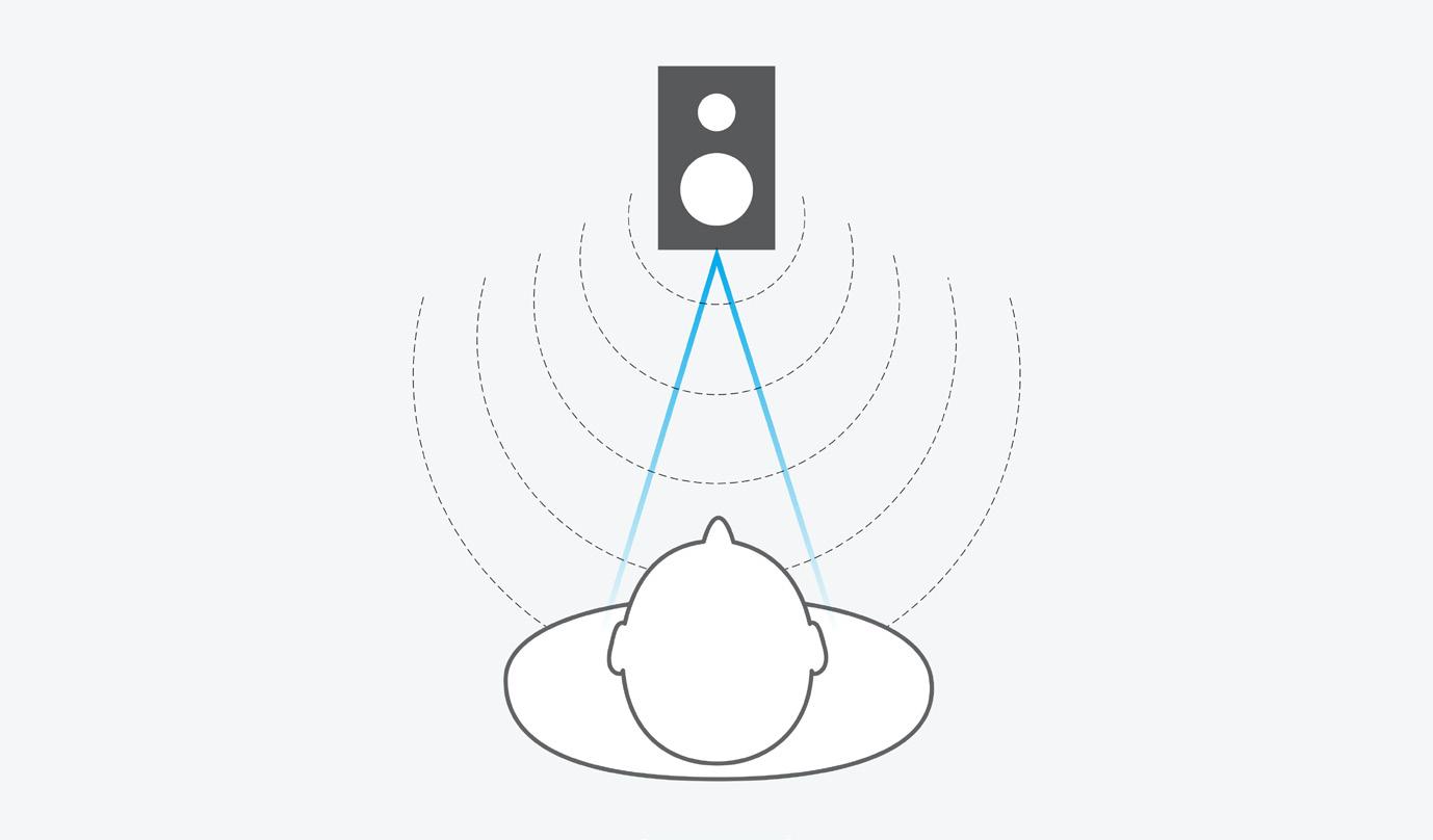
Sound waves emitted from a sound source directly in front of the listener arrive at both ears at the same time because the paths lengths are identical.

Sound waves emitted from a sound source to one side will arrive at the closer ear before the more distant ear because the paths lengths are different.

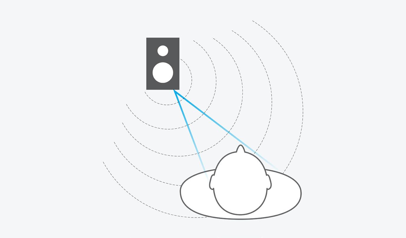
the brain can work out whether the sound source is located towards the left side or the right, based simply on which ear detects it first.

Moreover, by examining that timing difference more critically, the brain can calculate the angle of sound incidence with surprising accuracy. The diameter of an adult’s head is typically between 19 and 22 centimetres, which means, for a sound source at 90 degrees, the maximum time difference between sounds arriving at each ear is about 0.67 milliseconds. Lab tests suggest that the brain can detect differences in arrival times down to around 0.01ms (10 microseconds) — this is what gives us an angular resolution of about two degrees.

This ITD calculation is thought to be derived mainly from transients within the sound signal, which is probably why it’s often quite difficult to locate sound sources without transients — pure sine-wave tones, for example. For periodic signals like these the brain has to use phase differences between the two signals instead. However, the maximum

ITD of 0.67ms corresponds to a frequency of 1.5kHz, where the complete wavelength is roughly the same as the diameter of the average head. So, signals with fundamental frequencies higher than this will arrive at the distant ear with a phase difference greater than 360 degrees, and this inevitably creates confusion and ambiguous locational information because a phase difference of 405 degrees looks the same to the brain as one of 45 degrees (45 + 360 = 405), Thus, for periodic signals the ITD method is only reliable at frequencies well below 1.5kHz.

Inter-aural Level Differences

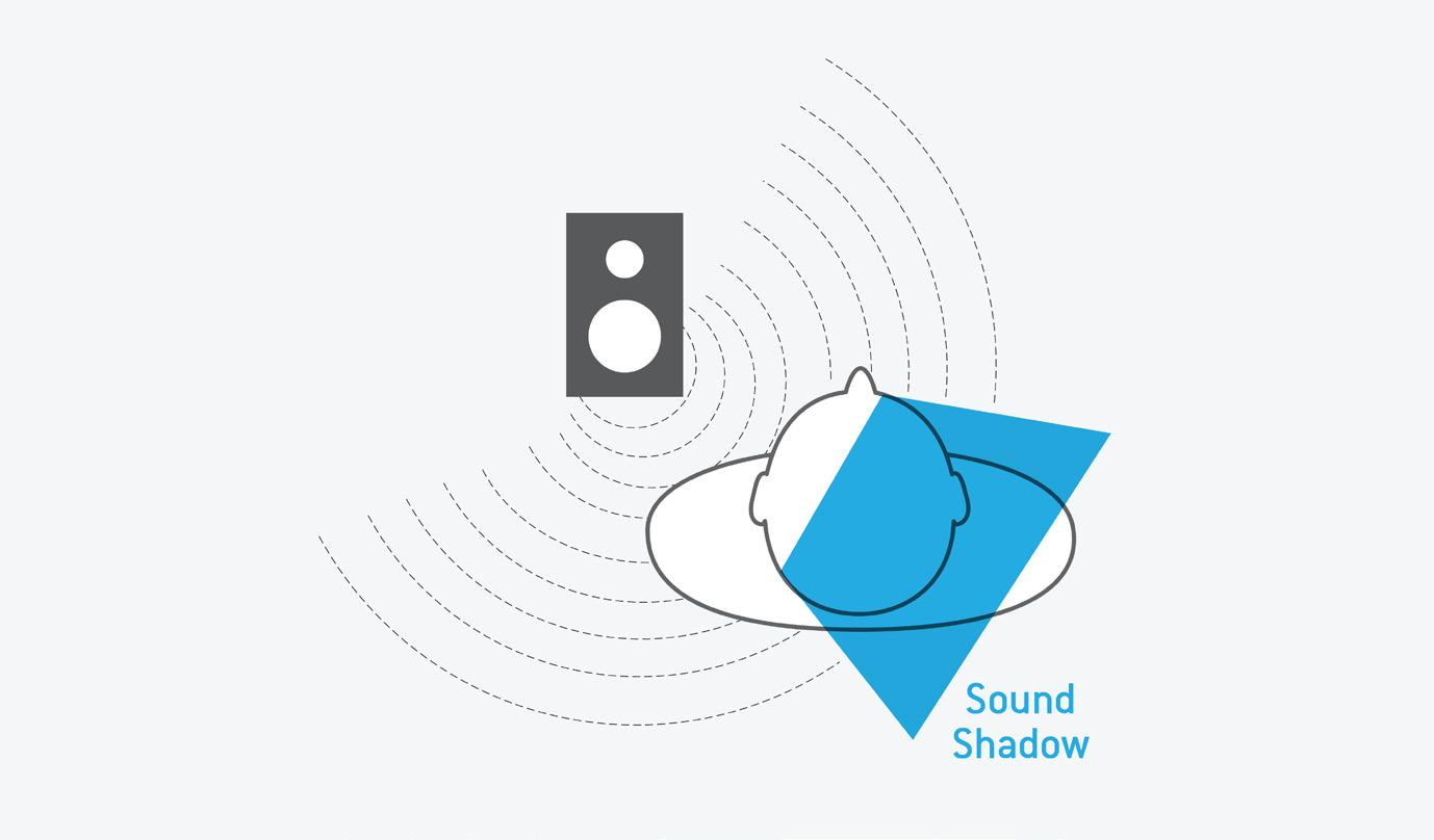
The second methodology, Inter-aural level differences (ILDs), is caused mainly by us having an acoustic ‘baffle’ between the ears — otherwise known as a head! At higher frequencies (above about 1.5kHz, where the wavelength approaches the diameter of the average head), this causes a ‘sound shadowing’ effect for the distant ear. Consider a sound source directly in front of a listener, again: the

sound level of high frequencies reaching both ears will be the same, because there’s nothing in the way between the source and ears to affect the sound level. If that source moves off to one side again, while remaining at the same distance from the closest ear, the level at that closer ear will remain the same. However, the level at the distant ear will be reduced slightly because the sound waves diffract around the head, creating a ‘sound shadow’. The actual amount of signal-level reduction is a function of both the angle of incidence and the source frequency; the attenuation due to diffraction increases as the frequency rises and the wavelength decreases.

These two primary sound localisation systems, ITDs and ILDs, function largely independently of each other. In experiments using headphones, though, it’s possible to use a delay at one ear, creating a contradicting ITD, to overcome the perceived source direction generated by an ILD. That’s an effect that can’t happen in real

As high-frequency sound diffracts around the head a sound shadow is created, reducing the level reaching the distant ear.

life, of course, but it does illustrate just how easily the brain can be fooled! Importantly, turning the head towards a sound source will always reduce both the ITD and the ILD (turning away increases both), which is another important aid used by the brain to deconflict ambiguities and bring the sound source into sight. This is why people often unconsciously tilt or turn their heads when listening to something intently: it’s an automatic response.

Spectral Distortions

The third location-detection process, spectral cues, is about decoding complex spectral distortions that are created by interference patterns occurring between the directly arriving sound waves and reflections off the shoulders and from the curves of the pinnae. Essentially, these are unique comb-filtering response dips, and these high-frequency interference patterns vary with the angle of sound incidence (both horizontally and vertically). They are absolutely unique to each individual, too, because they are wholly

dependent on the exact shape of the outer ears and other aspects of the person’s physique. In early life, the brain learns to correlate these unique spectral distortions with known sound-source locations, and the individual gradually develops the ability to locate sound sources just through recognising specific spectral distortion patterns.

Interestingly, whereas ITDs and ILDs are both binaural hearing processes (meaning the brain makes use of both ears to evaluate the sound direction), spectral cues are entirely monaural — the sound source location can be calculated from the spectral distortions to sound waves detected using a single ear! More importantly, spectral cues are particularly important for resolving front/back confusions and source

locations in the vertical plane, which ITDs and ILDs can’t differentiate at all.

Monaural Location

This mechanism explains how deafness in one ear doesn’t destroy the ability to locate sound sources. If you’d like to test it, try lying in bed with your eyes shut and one ear buried in a pillow (thus removing the option for binaural hearing) as a partner or child enters the room and moves around the bed. You’ll find you can estimate their position in the room with surprising precision, even without binaural hearing!

And, if you think about it, one reason headphone listening can sound artificial, with sound sources perceived as being inside the head rather than in the space around it, is that these spectral cues are

“Spectral cues are entirely monaural — the sound source location can be calculated from the spectral distortions to sound waves detected using a single ear!”

inherently absent; the sound is essentially injected straight into the ear canal without the benefit of reflections from the pinnae and shoulders. This missing information confuses the brain into deciding sounds must be ‘inside the head’. Even with true ‘binaural recordings’ — I’ll be discussing those in chapter 9 — the perceived ‘outside the head’ sound locations are often variable for different listeners.

These ‘problems’ can be addressed very effectively using crossfeed matrix processing, which simulates the natural ‘crosstalk’ of sounds arriving at both ears in the real world, and personalised Head-related Transfer Functions, or HRTFs. HRTFs are a set of spectral (frequency) modifications that are applied to the binaural signal, to simulate different intended sound-source locations. But, while generic HRTFs can

certainly be helpful, if we’re to perceive accurate and stable image locations we require HRTFs that are designed specifically for each individual — that’s because we each have uniquely shaped pinnae and different physiques. Thankfully, technology is starting to make that a lot easier to achieve, with quite good results coming from analysing photographs of an individual’s ears, for example!

Auditory Cues, Mics & Loudspeakers

So, our ears and brain derive the location of a point-source sound through ITDs, ILDs and spectral cues, and we try to recreate that information by using two loudspeakers spaced apart, preferably at ±60 degree angles to our listening position. What could possibly go wrong? Amazingly, this peculiar scheme works well, fooling

our ears/brain into creating ‘phantom sound sources’ that appear to be positioned somewhere in the space between the speakers. Technically, it recreates the sound wavefronts required to work very well at low frequencies (below about 700Hz), where level differences between the two speakers create accurate ITDs at the ears (that’s right, time differences! More on that in chapter 2...). At higher frequencies, the system doesn’t work quite so well and, in effect, creates spatial aliases that smear the soundstage and reduce imaging accuracy.

For stereo recording, the microphones are tasked with capturing ILD and/or ITD information in lieu of our own ears, and different stereo mic techniques achieve that in different ways. I’ll be looking at these, and delving into the mysterious workings of stereo loudspeakers, in the chapters that follow.

Chapter 2 Emulating The Real World

The

earliest attempts to convey a natural sense of sound positioning over speakers led to coincident mic techniques that remain popular today.

In chapter 1, we looked at the intentions behind recording in stereo, and how the human ears/ brain work out the location of an audio source in the real world, using three primary mechanisms: inter‑aural level differences (ILDs), inter‑aural timing differences (ITDs), and spectral cues from the sound reflections off the shoulders and pinnae.

The reason why we needed that background information is that, when we capture and replay stereo recordings, our aim is to recreate those auditory locational cues, either as accurately as possible, or in a way that is pleasingly believable. So, before moving on to examine different stereo microphone techniques, we need to consider how the ways in which we audition two channel stereo recordings emulate the real world experience. And for that, we need to look in particular at the pioneering work in the 1930s of Alan Dower Blumlein.

Until such time as humans can be upgraded with direct Bluetooth reception to the auditory processing centre in the brain, we only have two options for listening to stereo recordings: loudspeakers or headphones/ earbuds. Both approaches have their merits and disadvantages, but they each interface with the

human hearing system in dissimilar ways, so they result in significantly different experiences.

By their very nature, headphones and earbuds isolate each ear, so each can only hear the signal presented via its own channel. This is in contrast to real life, where both ears always hear a sound source, but with different levels, timings and frequency responses, as previously explained. So this aural exclusivity is inherently unnatural, and the most obvious result is where sounds are perceived as existing within the head — along an imaginary line between the ears, rather than in the space around us. There are ways to resolve that problem, though, and I will return to that later.

In the meantime, listening over loudspeakers is where stereophony began, and the majority of stereo microphone configurations are

optimised for this format — so that’s where we’ll start.

Loudspeaker Stereo

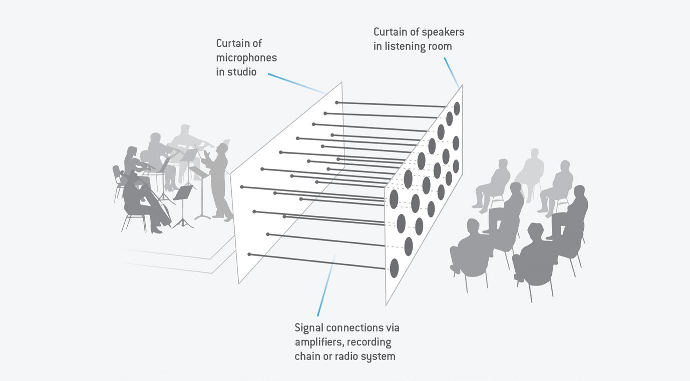
To most people, ‘stereophonic’ implies two loudspeakers, but it wasn’t always that simple. Back in the early 1930s, Dr Harvey Fletcher and his team, working for Bell Labs in America, were experimenting with multi‑channel sound recording and reproduction. His initial work used a large curtain of many microphones, arranged laterally and vertically in front of a stage, effectively sampling the combined sound wavefront projected from an ensemble on that stage. Each of those microphones was linked individually (via suitable gain stages) to a correspondingly located loudspeaker in a separate listening room, the idea being to reconstruct the original sound wavefront, preserving all directional information

Fletcher’s Curtain of Sound.

from the sound sources on stage — a system that was known as the ‘Curtain of Sound’.

This system actually worked very well, but of course it was highly impractical — especially since multi-channel recording and transmission hadn’t yet been invented, from the recording and transmission points of view! Fletcher and his team therefore simplified the system, eventually deciding that three microphone/ loudspeaker channels, arranged as left, centre and right, in a horizontal line, was the minimum arrangement for recreating acceptable locational information. To demonstrate this new format to the public in March 1932, Fletcher arranged a live relay, using telephone lines to route the three audio channels from the Academy of Music in Philadelphia to the Constitution Hall in Washington. The Conductor in Philadelphia was Leopold Stokowski, who had a great interest in improving recorded sound, and he went on to help Disney develop their bespoke surround-sound system, Fantasound, which was launched in a roadshow

“Blumlein... realised that recreating the original source time-of-arrival differences from three loudspeakers, as Fletcher was doing in America, had serious inherent problems.”

tour of the Fantasia film to public theatres across the USA in 1940.

The results of Fletcher’s public demonstration were considered impressive, but the technical difficulties of managing even three channels — maintaining their critical phase, timing and level relationships — eventually curtailed further development. From a commercial perspective, another significant problem was how to create a mono recording for release on a 78rpm disc. Downmixing all three mic channels to mono resulted in unpleasant comb-filtering, while only using the centre channel lost information from the sides, compromising the overall balance. Solutions were found in time, of course, most notably with the superb Mercury Living Presence recordings made by Robert Fine in the late 1950s and early ’60s.

Meanwhile, in the early 1930s in the UK, Alan Blumlein was working for EMI on sound recording and reproduction techniques. He realised that recreating the original source time-of-arrival differences from three loudspeakers, as Fletcher was doing in America, had serious inherent problems, and chief amongst them was that both of the listener’s ears could hear signals from all the loudspeakers. Consequently, the intended time-of-arrival differences captured by the stage microphones were subsequently confused by the additional time-of-arrival differences created by each of the replay loudspeakers. Moreover, these additional ITDs are dependent on the position of the listener relative to the speakers, which makes life difficult in theatre settings with lots of listeners.

It occurred to Blumlein that this apparent problem of each ear hearing all loudspeakers could potentially be used to advantage — but only if he gave up the idea of capturing the real time-of-arrival differences from the sources. His new scheme relied on reproducing only intensity (amplitude) differences between the signals feeding each loudspeaker, a system that creates an illusion of directional sound information with remarkable realism and stability.

Blumlein called his invention Intensity Stereo. To work with reasonable accuracy, it requires the speakers and listeners to be positioned at the points of an equilateral triangle (ie. with a 60-degree listening angle). This arrangement fools the ear/ brain into translating the pure level differences between signals from the two loudspeakers into artificial ITDs, portraying spatial information about (virtual) sound source positions arrayed between the two loudspeakers. This brilliantly clever solution is explained in the ‘Stereo Illusion’ side box in this chapter.

It’s worth noting in passing that Intensity Stereo is not the only way to create the impression of different spatial positions. A similar effect can be created by introducing small delays into signals of identical levels reproduced from each loudspeaker — and that’s something we’ll come back to later.

Coincident Microphones

Having come up with a workable system to create the illusion of virtual sound sources positioned in space between a pair of loudspeakers, the logical next question was how to capture the positioning of real sound sources on a stage and convey that information to the loudspeakers as an Intensity Stereo signal.

The critical aspect here is that timing differences between the channels are expressly not required, so separate, spaced microphones like Fletcher was using are not acceptable. Instead, the

two microphones feeding the two channels must receive all sounds at exactly the same time. That means the mics must occupy the same point in space — in words more familiar to recording engineers, they must be coincident in space. Also, to create suitable amplitude differences in each channel, proportional to source stage positions, the microphones require directional polar patterns, and must be aimed in different directions.

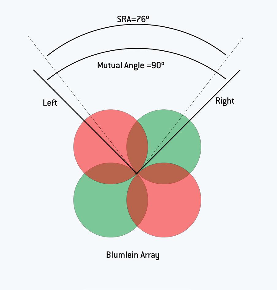
In the 1930s, microphone polar pattern options were relatively limited, with figure-8 ribbon mics being the best option for Blumlein’s coincident microphone experiments. That resulted in the stereo mic array that has acquired his name: the Blumlein array comprises two figure-8 mics mounted vertically, one above the other, such that they are coincident in the horizontal plane. One mic is typically arranged to face 45 degrees left, and the other 45

degrees right, such that the mutual angle between them is 90 degrees (although, as I’ll discuss in the next chapter, other options are available).

A central sound source in front of these coincident microphones will be captured at the same time and the same level (albeit off-axis) in both, thus creating a central phantom image when auditioned on loudspeakers. If the sound source moves to the left, it will move more on-axis to the left-facing mic, and more off-axis to the right-facing mic, so creating a level difference between the two channels, being louder on the left. This level difference creates a corresponding image position when heard on loudspeakers.

When the sound source is directly on-axis to the left microphone, it will also be directly in the null of the right microphone, so virtually all the signal will be in the left channel (ignoring any reverberation) and the sound will

“A TF11 Stereo Set is a great choice on anything from drums and piano to vocals. It adds a nice sweetness to anything you put in front of it.“

- Brenden Morawski

*Alicia Keys, Ariana Grande, Charli XCX*

TF11 FET STEREO SET

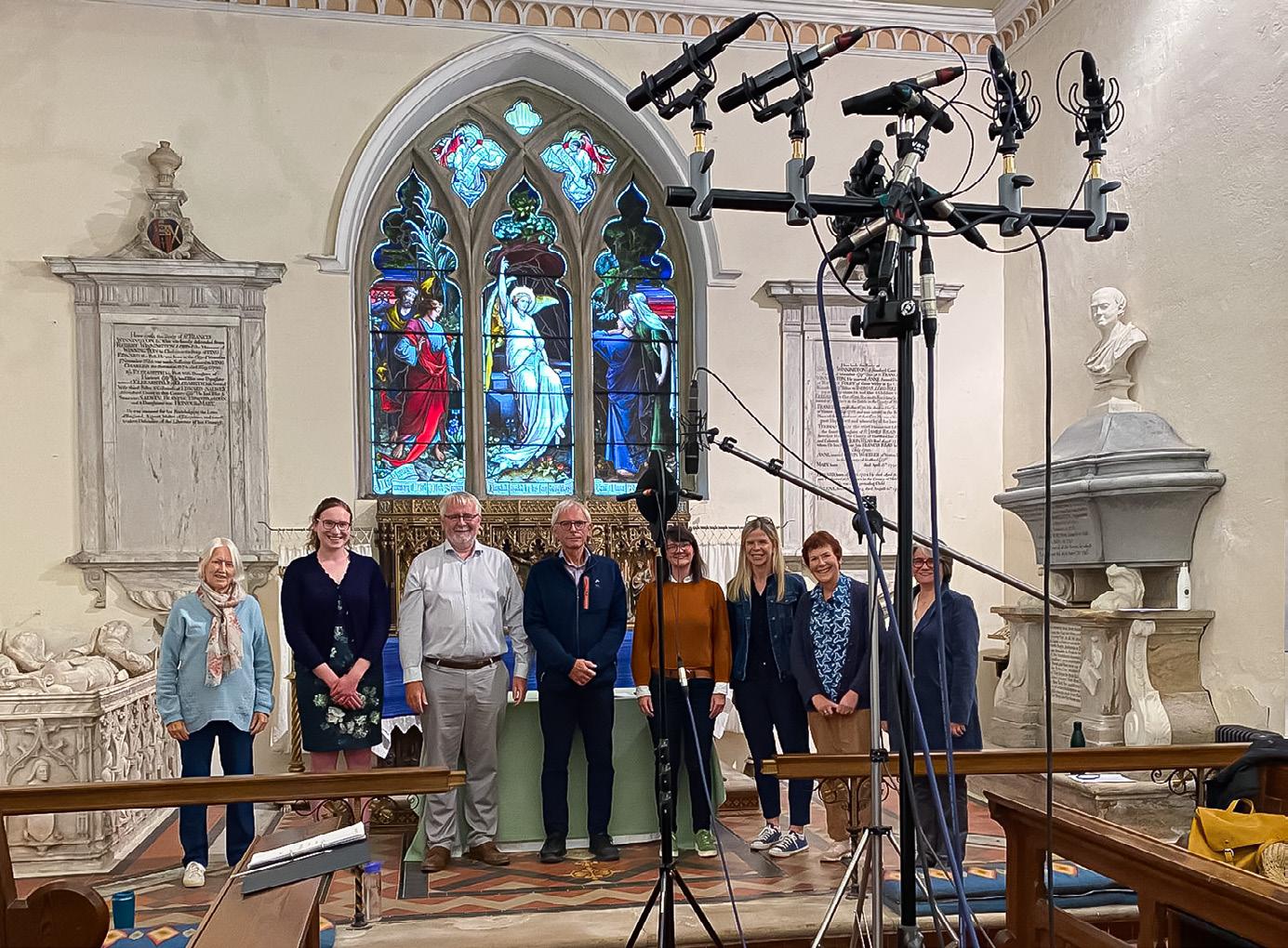
The Teme Valley South Churches Choir (TVSCC), who kindly repeatedly performed ‘If Ye Love Me’ by Thomas Tallis, to help us demonstrate the different stereo mic arrays.

therefore emanate only from the left loudspeaker. So, this arrangement creates a stereo recording angle or ‘SRA’ in front of the microphones — a region being recorded which is effectively ‘mapped’ into the available space between the two loudspeakers during replay.

In the case of the Blumlein array as described, that SRA is about 76 degrees, but every different stereo mic array will have a specific SRA value. Again, much more on that in the next chapter, but for now, this SRA value matters because the sources you wish to record have to be contained within the mic array’s SRA if they are to be portrayed with reasonably accurate relative locations from the loudspeakers.

Listening

To illustrate the strengths and weaknesses of different stereo

mic arrangements, I’ve prepared a series of demonstration recordings that you can find on the SOS website at https://sosm.ag/stereo miking demo files. Over about an hour on a warm summer’s evening, I recorded the Teme Valley South Churches Choir (TVSCC), founded and conducted by Chloe May Evans, in a hilltop church in Worcestershire, UK. I am immensely grateful for their generosity and patience as this required them to perform the same piece repeatedly in front of a number of different mic arrays, some being reconfigured or physically moved between takes! A detailed explanation of these audio files can be found on p72.

I’ll describe more of these recordings, and their specific points of interest, in later chapters, but for now I suggest that you listen to the first track. Captured

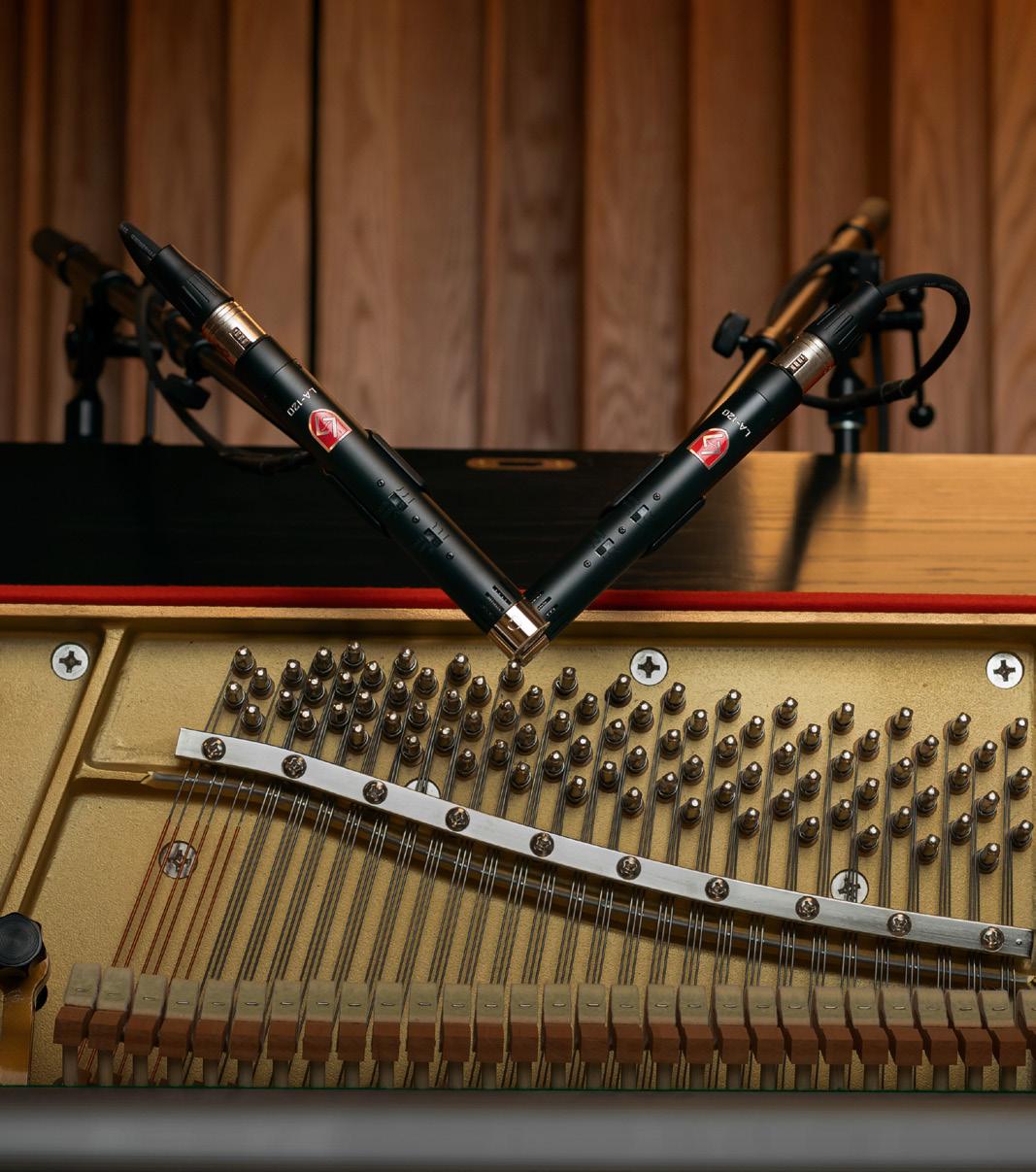
with a Neumann SM69 FET single‑bodied stereo mic, set up as a Blumlein array of figure 8s with a mutual angle of 90 degrees, this arrangement captures sound from the mics’ rear lobes in addition to the front ones, and that adds to the overall room reverberation, while reverberant sound arriving at the sides is captured in opposite polarities by both mics, adding to the sense of spaciousness. Although not apparent here — the small choir were positioned in a single line — this mic array is also particularly good at portraying stage depth in a realistic manner.

In the next chapter, I’ll continue to explore coincident mic techniques, compare their strengths and weaknesses, and look at some useful practical tools for choosing and optimising different arrays.

Stereo Illusion

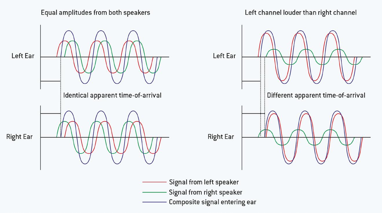
Blumlein’s revolutionary invention of Intensity Stereo is ingenious, but the concepts can be explained simply by considering steady sine‑wave tones being reproduced by each loudspeaker — yes, I realise I said in chapter 1 that it’s hard to locate steady tones in real life, but it’s much easier to follow the theory if we use sine waves! Let’s start with an identical sine tone reproduced at identical levels by both loudspeakers, as illustrated in the diagram above. The left ear receives the signal from the (closer) left speaker first (red wave) and then from the right speaker (green wave) a short time later.

The reverse happens in the right ear, of course, but, since the listener is at the apex of an equilateral triangle, with the speakers at the other two points, the distance between right ear and right speaker is the same as the distance from left ear to left loudspeaker. Consequently, the right speaker signal arrives at the right ear at exactly the same time as the left speaker signal arrives at the left ear. A few microseconds later, each ear hears sound from the more distant speaker. Now, the two signals arriving at each ear will sum together acoustically as they arrive at the ear drum — that result is shown as the blue wave for each ear. As the signals from both loudspeakers have identical

levels, the resultant signal entering each ear will be identical, and its apparent starting time is exactly mid way between the real signals from each speaker. So, as far as the ear and brain are concerned, these two resultant signals (blue) have exactly the same time of arrival at both ears. Therefore, the virtual sound source is perceived to be directly in front of the listener — a ‘phantom’ central sound source.

If we now alter the relative levels of the signals produced by the two loudspeakers (which is easily achieved using a pan pot, for example), something rather magical happens. The illustration on the right shows that the signal from the left loudspeaker (red wave) is now much louder than that from the right (green wave).

When these signals combine as they enter the ear, the louder one dominates the sum, so the resultant signal appears to arrive earlier in the left ear than it does in the right. Again, as far as the ear/brain are concerned, we detect an ITD, which we perceive as a sound source to the left of the listener — its exact position is dependent only on the relative levels of signals from the left and right loudspeakers. As a rough guide, a level difference of 16dB is sufficient to create the illusion that a sound source is located firmly at a loudspeaker, while

a 4dB difference moves the source from the centre to about a quarter of the way across from the centre towards the louder speaker, 8dB about half way, and 12dB about three quarters of the way.

In other words, relative level differences (ILDs) between the signals reproduced by two loudspeakers are translated automatically into time of arrival differences (ITDs) at the ears, creating the illusion of virtual sound sources spread across the 60‑degree angle between the two loudspeakers.

Naturally, there are physical limits to the creation of stable stereo imaging, and the most obvious occur if the listener moves away from the apex of the equilateral triangle — the listening sweet spot, as we sometimes call it. Staying central but moving further back reduces the perceived ITDs, so the stereo image narrows. Conversely, moving forward, inside the triangle, increases the ITDs. This stretches the image wider, but also makes the phantom centre unstable. Moving to the left or right greatly exaggerates the perceived ITDs, and eventually the Haas effect takes over, whereby the brain latches onto the sound source it hears first — the nearest loudspeaker — and the stereo imaging collapses into the single speaker.

Just how much scope do you have to manipulate the perspective obtained using coincident mic pairs?

Chapter 3 Position & Perspectives

In the previous chapter, I explained how Alan Blumlein invented Intensity Stereo in the early 1930s, and that its key innovation was that differences purely in amplitude between signals, fed to two loudspeakers placed at two points of an equilateral triangle, could be converted into inter-aural time differences (ITDs) for a listener located at the triangle’s third point. Many people argue that this concept and implementation is the true origin of stereophony but, as we progress through the chapters that follow, we’ll see that most modern recordings actually push Blumlein’s theoretical boundaries quite a long way! Nevertheless, there is still more that we should explore within Blumlein’s Intensity Stereo idea...

We closed the last chapter with a description of Blumlein’s initial setup, using coincident (aka X-Y) figure-8 microphones set with a mutual angle of 90 degrees, and I explained how that arrangement gave a Stereo

Recording Angle (SRA) of about 76 degrees. Remember the significance of the SRA: sound sources arranged within that 76-degree region in front of the microphones in the recording environment are ‘mapped’ onto the 60-degree angle between the loudspeakers in the replay environment, and their relative positions are preserved in the stereo image.

To demonstrate this microphone arrangement, I recorded a small choir using coincident figure-8 mics set up in the Blumlein format (audio example 1 in the accompanying files: https://sosm.ag/stereo-mikingdemo-files), with the choir arranged to almost fill a 76-degree arc in front of the microphone. If you listen to that track on loudspeakers in a reasonably well-treated acoustic, the choir should be spread almost fully across the sound stage, and with quite clearly focused images of each singer; hopefully, you should feel as if you could point

at each individual voice. In fact, this impression of precise, focused sound positioning within the stereo image is a major strength of most coincident microphone techniques. If I were to offer a visual analogy, I’d suggest a comparison with a photorealistic painting, for example.

Perspectives

However, stereo recording is about much more than just the left-right imaging; the perspective of sound sources is critically important too. By ‘perspective’, I mean the perceived distance or depth of each singer within the full sound stage, and the balance between direct and reverberant sound.

In example 1, the (empty) church is quite reverberant, yet the captured perspective is quite acceptable in the context of the Tallis piece I recorded. But what if we wanted a drier and closer sound? That would obviously require the microphones

to be moved closer to the choir. But if we were to do that, the singers at the outer edges of the choir would be outside of the 76‑degree SRA of the Blumlein array.

The audible result depends on just how far outside the SRA the outer singers become, but at best they would appear bunched into the loudspeakers, and at worst they would be captured with opposite polarities in each channel, and thus attenuated, upsetting the balance in a mono downmix and appearing rather phasey and unfocused in stereo. In other words, the positional information within the stereo image would become distorted compared to the actual source positions in front of the microphones — a little like the optical distortion you see when a very wide angle camera lens is placed close to the subject.

To maintain a representative spread of singers across the full stereo image in a closer perspective, a much wider SRA will be required — this way, we can accommodate the greater stage width relative to

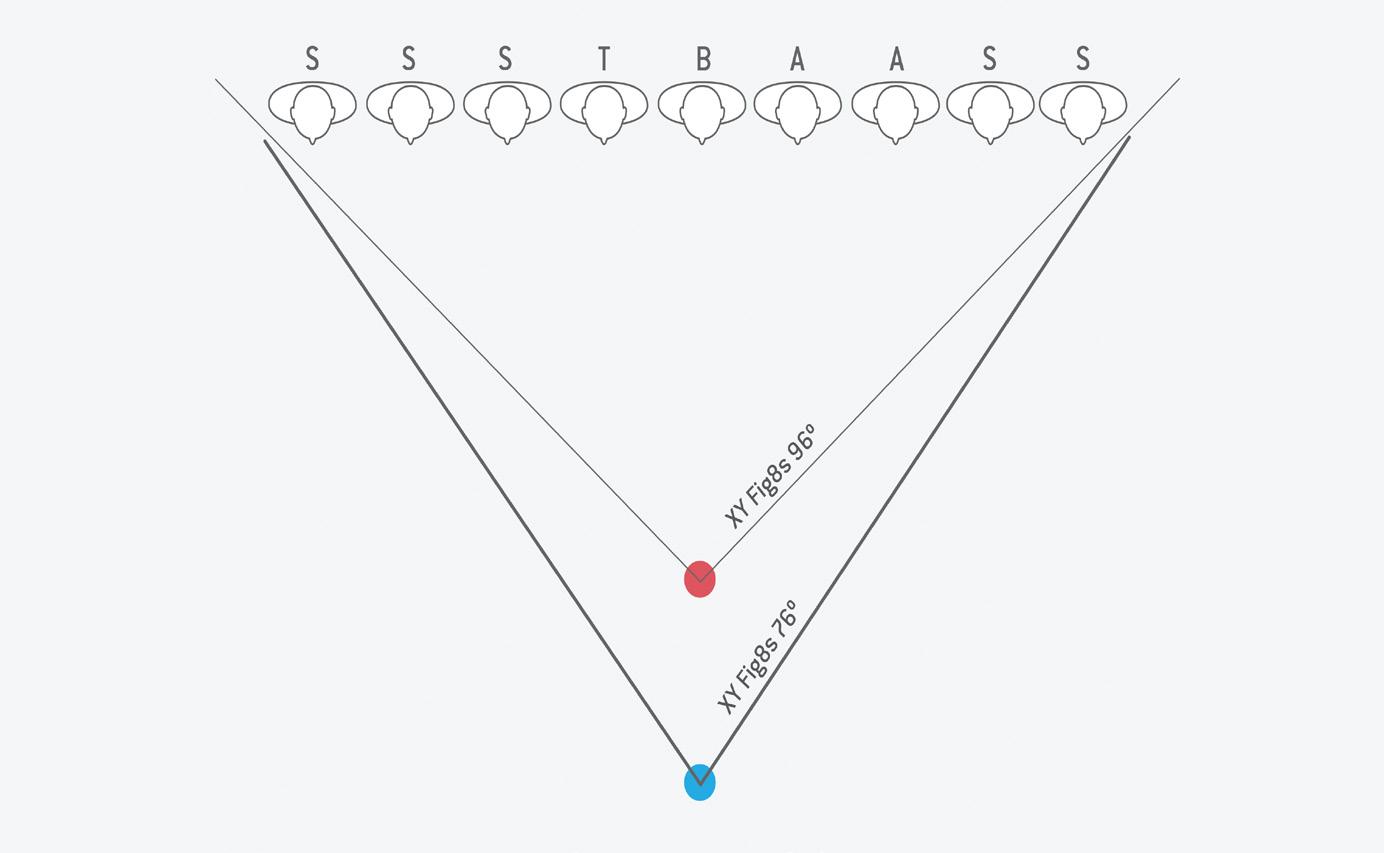
the microphone’s closer position — and, fortunately, there are a couple of ways of achieving a wider SRA. The first is to alter the mutual angle of the microphones. For example, by angling the mics inwards (ie. reducing the mutual angle), achieving a given amplitude difference between channels (and thus establishing a specific stereo image position) requires sound sources to move further away from the centre line than before — so the SRA is increased. This gives us Rule 1, when it comes to tweaking stereo mic arrays: reducing the Mutual Angle increases the Stereo Recording Angle.

Applying this idea to our Blumlein array, if the mutual angle of the microphones is reduced to 70 degrees (instead of 90) the SRA increases to 96 degrees. That wider SRA allows the mics to be moved closer to the choir, giving a drier perspective, but with the stereo image still spread nicely between the speakers without bunching at the edges, as shown in Diagram 1. Note, though, that while in this case

a 20‑degree reduction in mutual angle provides a 20‑degree increase in SRA, the proportions vary with other stereo mic arrays. For example, reducing the mutual angle of X Y cardioids by 20 degrees causes a 30‑degree increase to the SRA.

Of course, there’s only so far you can realistically reduce or increase the mutual angle before other imaging and tonality complications start to intrude...

Other Polar Patterns

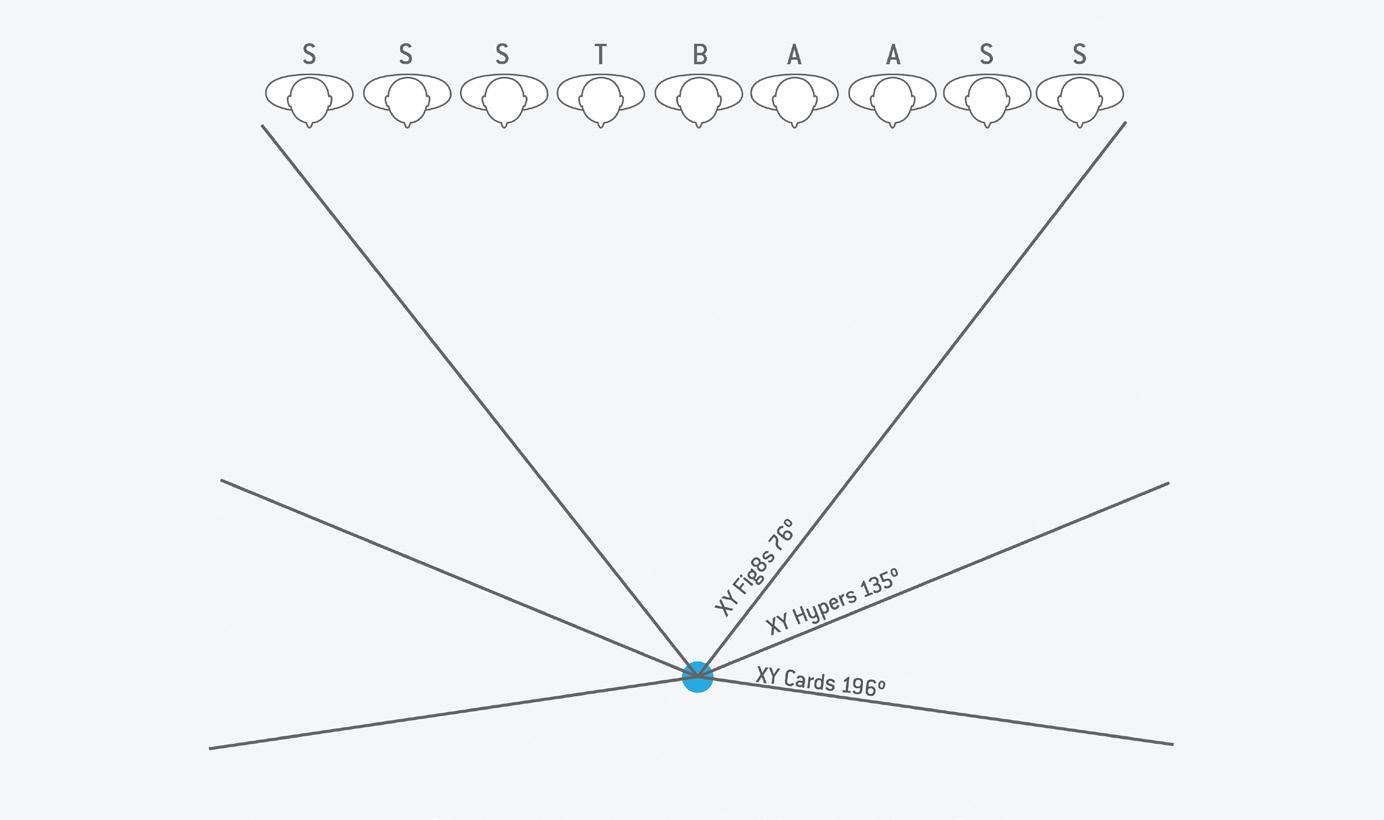
An alternative option is to keep the 90‑degree mutual angle, but change the microphone polar patterns to some other directional shape instead, such as hypercardioid or cardioid. Since these patterns have much broader frontal pickup regions than figure 8s, a sound source will need to move even further away from the centre line to generate a significant amplitude difference between the channels, and so these polar patterns inherently have wider SRAs. The extreme would be coincident omnidirectional

microphones, which would have an SRA of 360 degrees (and no stereo imaging at all — everything would appear to be in the phantom centre!).

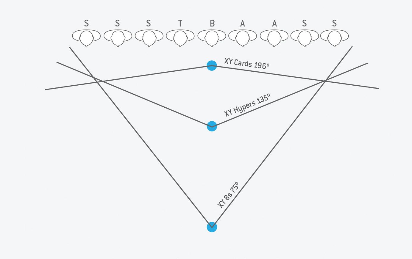
Diagram 2 compares the SRAs for coincident figure-8s, hypercardioids and cardioids (all coincident, with a mutual angle of 90 degrees). These configurations deliver SRAs of approximately 75, 135 and 196 degrees, respectively.

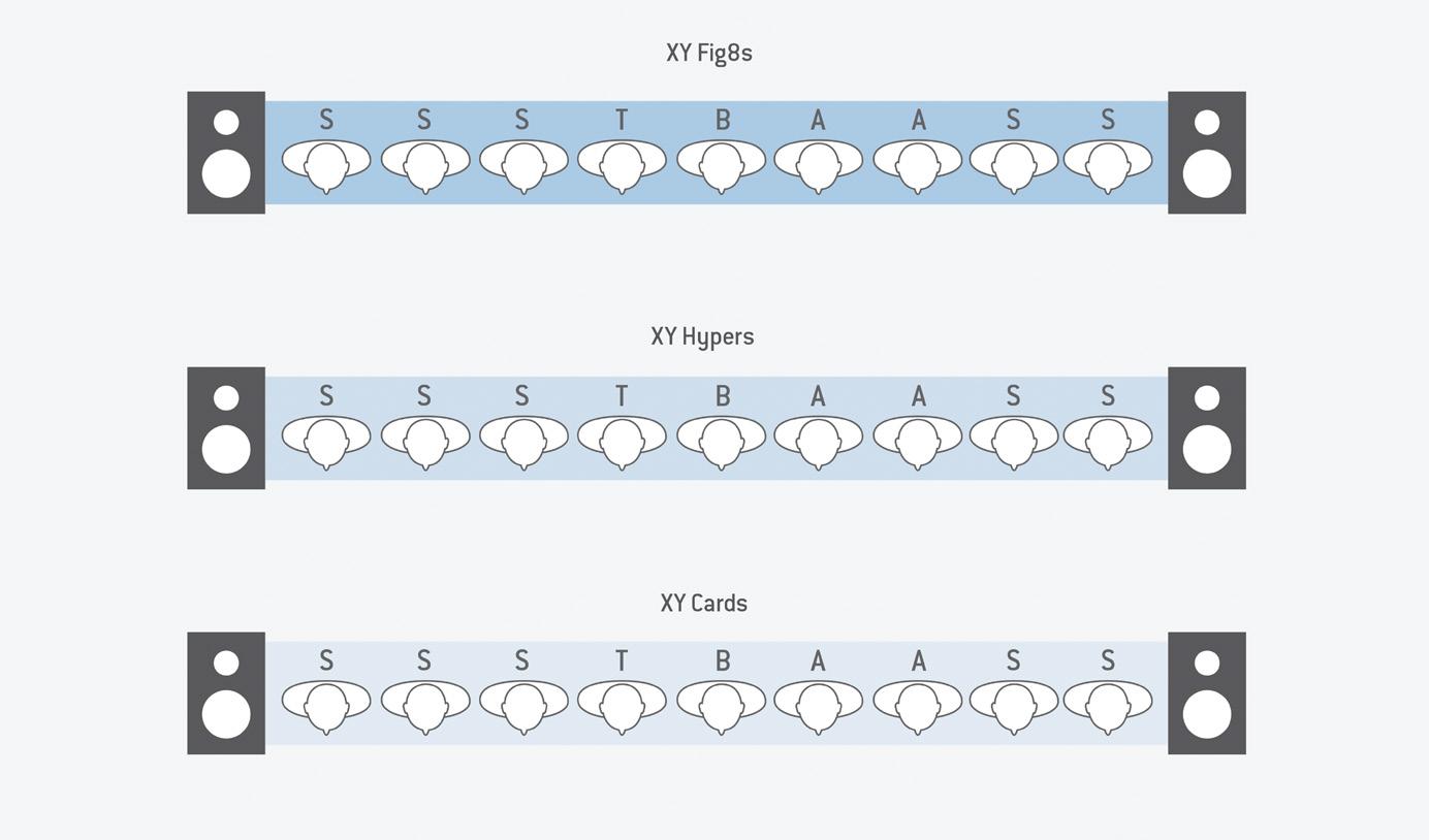
So, if the stereo microphone array stays in the same physical location, but the polar patterns are adjusted between those three options, the changing SRA alters the perceived stereo width of the choir because it then occupies a different proportion of the resulting SRA, as shown in Diagram 3. If the choir fully occupies the stereo image width with the figure-8s Blumlein array, it will be a little narrower with the hypercardioids, and a lot narrower with the cardioids. Note that the room’s reverberation always fills the entire stereo width in all three cases (shown here as the purple background).

The first three audio examples demonstrate these changing image widths with different microphone polar patterns. Example 1 uses figure-8s, while for example 2 the mics were switched to hypercardioids, and for example 3 to cardioids. Note how the church acoustic fills the space between the monitor speakers in all three examples, but that the choir occupies a reducing portion of the image width as you compare figure-8s to hypercardioids and cardioids.

The relatively strong reverberation in these demonstrations tends to make the difference less clear than in a drier acoustic, so for an alternative demonstration, example 13 is a recording I’ve borrowed from some stereo training material created in the BBC back in the late 1980s; I trust the BBC won’t mind me sharing it here in the interests of public education!

In this example another small choir is singing in a well-damped studio in front of a stereo mic (I suspect an AKG C422). The

microphone polar patterns were switched at 30 second intervals from cardioid to hypercardioid to figure-8, and I have inserted short tone bursts between the three sections to make their identification easier. The order here is the reverse of my church examples, so the image starts off fairly narrow with cardioids, then gets wider with hypercardioids, and finally fills the entire image width with figure-8s. Diagram 4 illustrates what you should hear as the track plays.

Choosing different polar patterns for the coincident stereo array allows for a much wider range of SRAs than can be achieved just by adjusting the mutual angle, giving far greater flexibility in positioning the microphones to achieve required perspectives. To demonstrate this, examples 4, 5, and 6 were also recorded with the Neumann SM69 FET microphone, but this time I changed both the mic’s physical position and its polar patterns to try and maintain a constant, full image width but with very different perspectives.

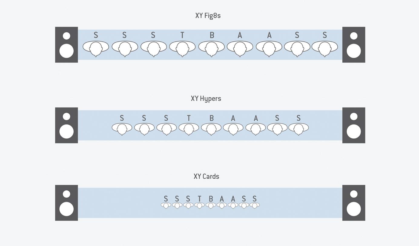
Diagram 3: While the width of the source might be different, the reverb fills the stereo stage in all cases.

As you’d expect, the balance is much drier for the cardioids placed very close to the choir (example 6), and far more reverberant with the figure-8s far away (example 4). The hypercardioids offer a half-way option (example 5), and Diagram

5 shows the relative mic locations. Diagram 6 is an attempt to indicate the perspective by showing the amount of reverberation as the purple background, with the darker colours indicating more reverberation or a more distant perspective, and the

lighter colour meaning less reverb and a closer perspective.

Pros & Cons of Coincident Mic Arrays

As I’ve already mentioned, the overwhelming strength of most

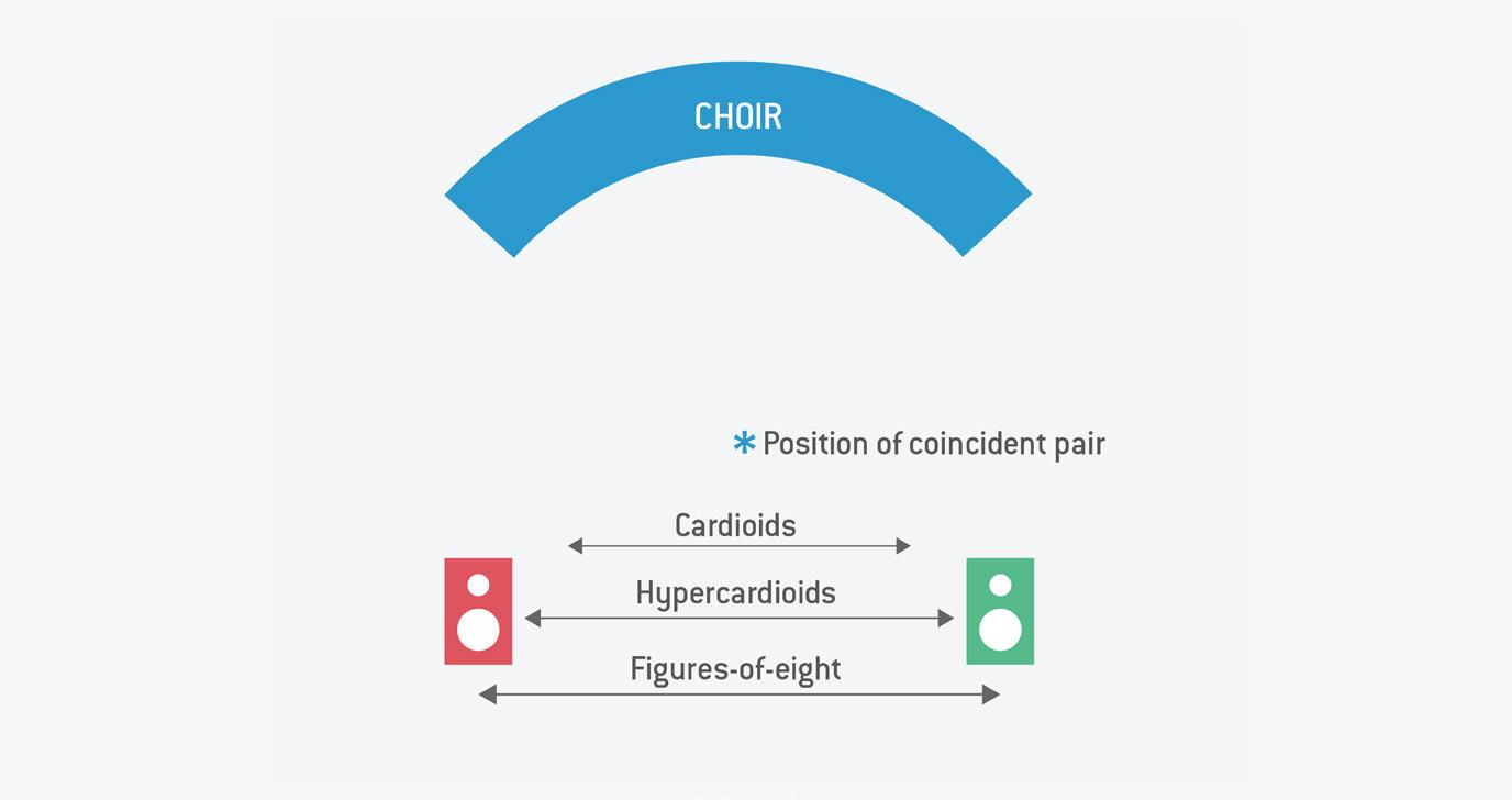
Diagram 4: An illustration of the differences you should hear when listening to audio example 13.

coincident mic arrays is the precision of stereo imaging — the focus, detail and stability. This is largely due to the X Y arrangement capturing only intensity or amplitude differences between the two channels, allowing the loudspeakers to convert them into ITDs (inter‑aural time differences) with very little ambiguity for the listener. So, coincident mic arrays are, without doubt, the optimal format for conventional stereo loudspeaker auditioning, if ultimate stereo imaging precision is the aim.

That said, not all X Y mic arrays are born equal! In particular, the coincident cardioids format is a challenge to employ because, with an SRA of around 196 degrees, it must be placed extremely close to the sound sources in order to fill the stereo image. Consider recording an orchestra, for example: to capture a full width image the stereo microphone array has to be placed directly above the conductor! The inevitable result in this case is that the front desks of strings will

“Not all X-Y mic arrays are born equal! In particular, the coincident cardioids format is a challenge to employ...”

be far louder than the more distant desks because of their relative distances from the mics, and so the overall balance of the orchestra is exaggerated, and additional mics are likely to be needed to allow a more natural balance to be achieved in a mix — with all the attendant problems that involves.

A coincident hypercardioid array doesn’t suffer from this exaggerated balance issue because its SRA of 135 degrees permits a more distant placement where the mics can ‘see’ all instruments at similar distances — and it’s the same for coincident

figure‑8s with a 76‑degree SRA, but here the even more distant mic array might be a problem in a very reverberant space.

Another aspect that counts against coincident techniques in general is that many listeners perceive them to lack a sense of ‘spaciousness’ or to be overly clinical, preferring instead systems which introduce some level of inter channel timing differences in addition to the inter channel level differences — a complex topic that I’ll explore in depth in a later chapter. This spaciousness aspect relates mainly to the degree of correlation between channels at low frequencies, and the cause is the divergence between theory and practice! In theory, a cardioid mic is cardioid at all frequencies, for example, but in practice it tends to become more omnidirectional at low frequencies (red outline in Diagram 7). The same is true for most directional microphones.

What this means is that a given sound source location might

create a certain inter-channel level difference at mid frequencies, but at lower frequencies where the polar pattern tends towards omni, the level difference becomes much less. So, the low-frequency components tend to be reproduced towards the centre of the stereo image, and this gives the impression of little spaciousness. Fortunately, this issue can be fixed, and I’ll return to suitable corrective processing in a later chapter, although the solution is based on another of Blumlein’s original ideas!

Interestingly, the real-world lack of directionality at low frequencies doesn’t apply to ribbon figure-8 microphones, which is perhaps why the original Blumlein array works so well and delivers such a reliably pleasing stereo sound.

Stereosonic Shuffling

Another common issue with real-world microphones differing from the theory is an extension of the same problem. Not only do many directional mics lose their directionality at low frequencies,

but they also tend to become more directional (or ‘beamy’) at higher frequencies (the blue pattern in Diagram 7). The effect is to generate increased inter-channel level differences at high frequencies compared with mid and low frequencies, which means that the high-frequency components of a sound source will appear to come from a wider position in the stereo image than lower-frequency components, effectively smearing the stereo image (Diagram 8). For another visual analogy, it’s a bit like a poor-quality camera lens where the red and blue light travels along slightly different paths through the lens, resulting in unintended colour fringing, making the picture look slightly blurred.

This exaggerated HF image width is compounded further by another real-world issue concerning stereo loudspeaker monitoring. The conversion of amplitude differences between the speakers to perceived time-of-arrival differences at the listener (Blumlein’s core Intensity Stereo concept that we discussed

in chapter 2) relies on both ears hearing the same level from both speakers, but at different times due to relative distances. That concept works perfectly at frequencies below about 700Hz, but above that frequency, the presence of the head between the ears causes some sound-shadowing, causing the sound level reaching the more distant ear to be slightly lower than it should be. Again, this results in a greater perceived time-of-arrival difference for high-frequency components, which therefore appear to be at wider locations than intended.

I’m sure Alan Blumlein would have addressed this complication if he’d had the chance, but he was seconded to work on the development of airborne RADAR during the Second World War, and his life was tragically cut short in an accident during airborne trials. However, his former colleagues at EMI did get to address it after the war, with a corrective system they called the Stereosonic Shuffler — a facility that was built into EMI’s

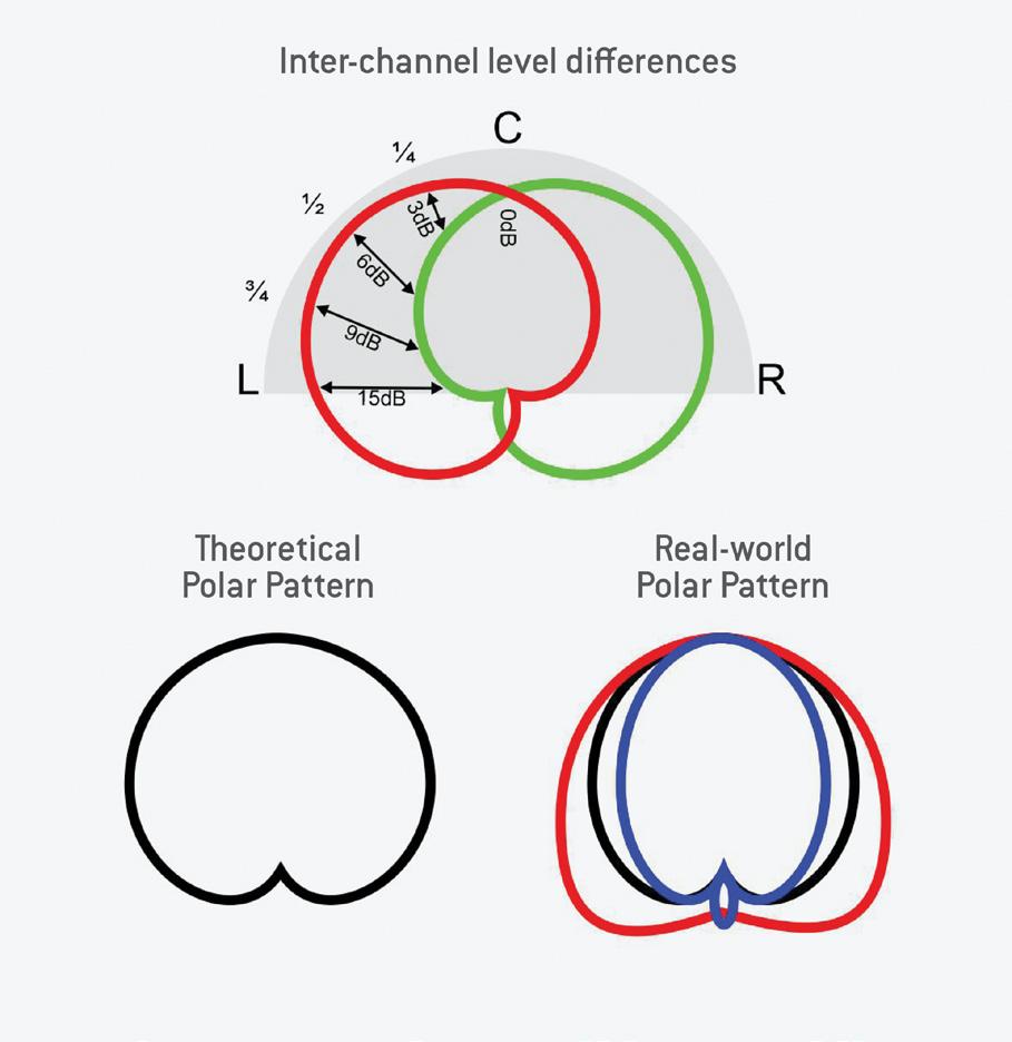
Diagram 7: A cardioid mic isn’t truly cardioid across all frequencies!

stereo mixing consoles through the 1950s and early ’60s.

I should clarify that there are at least two different forms of Shuffler: Blumlein created the first in the 1930s and I alluded to it above as a fix for the spaciousness problem;

it has been suggested that his former colleagues reused the term in his honour when they came up with the Stereosonic Shuffler, since it uses similar concepts. In simple terms, the Stereosonic Shuffler converts the left-right

stereo signal into the Mid-Sides format, and introduces around 3dB of attenuation into the Sides channel above 700Hz, before converting back to the left-right format. This processing has the effect of reducing the stereo image width at higher frequencies, thereby compensating both for the microphone polar pattern beaming effect in the recording stage and the head-shadowing effect in the listening stage. (If this Mid-Sides terminology furrows your brow, fear not; I’ll explain it in enormous detail in the next chapter!)

Sadly, the complexities of analogue Mid-Sides signal processing in the 1950s meant that EMI’s Stereosonic Shuffler introduced as many compromises as it fixed, and thus the idea had been abandoned by the mid-1960s. Today, UK niche manufacturers Phaedrus Audio currently make a product called the Shuphler that recreates the Stereosonic Shuffler process in a rather better-engineered way, avoiding the shortfalls of the original design. The same stereo processor also offers a variety of other stereo correction modes for different microphone and replay formats. It’s a unique and very interesting product which I’ll come back to later...

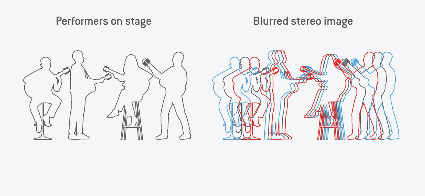
Diagram 8: Because of the increasing sensitivity of directional mics to higher frequencies arriving on‑axis, the stereo image can appear slightly blurred on playback. Thankfully, though, this can be addressed with a Stereosonic Shuffler process.

To conclude our primer on coincident arrays, we take you through the theory and practice of Mid-Sides miking.

Chapter 4 Mid-Sides Recording

In the previous chapter, we continued to explore coincident (X-Y) stereo microphone arrays, and looked at how the Stereo Recording Angle (SRA) can be altered, either by changing the mutual angle between the two mics, or by changing the mics’ polar patterns. But there’s another form of coincident mic array — the mysterious Mid-Sides format — and that’s the focus of this chapter.

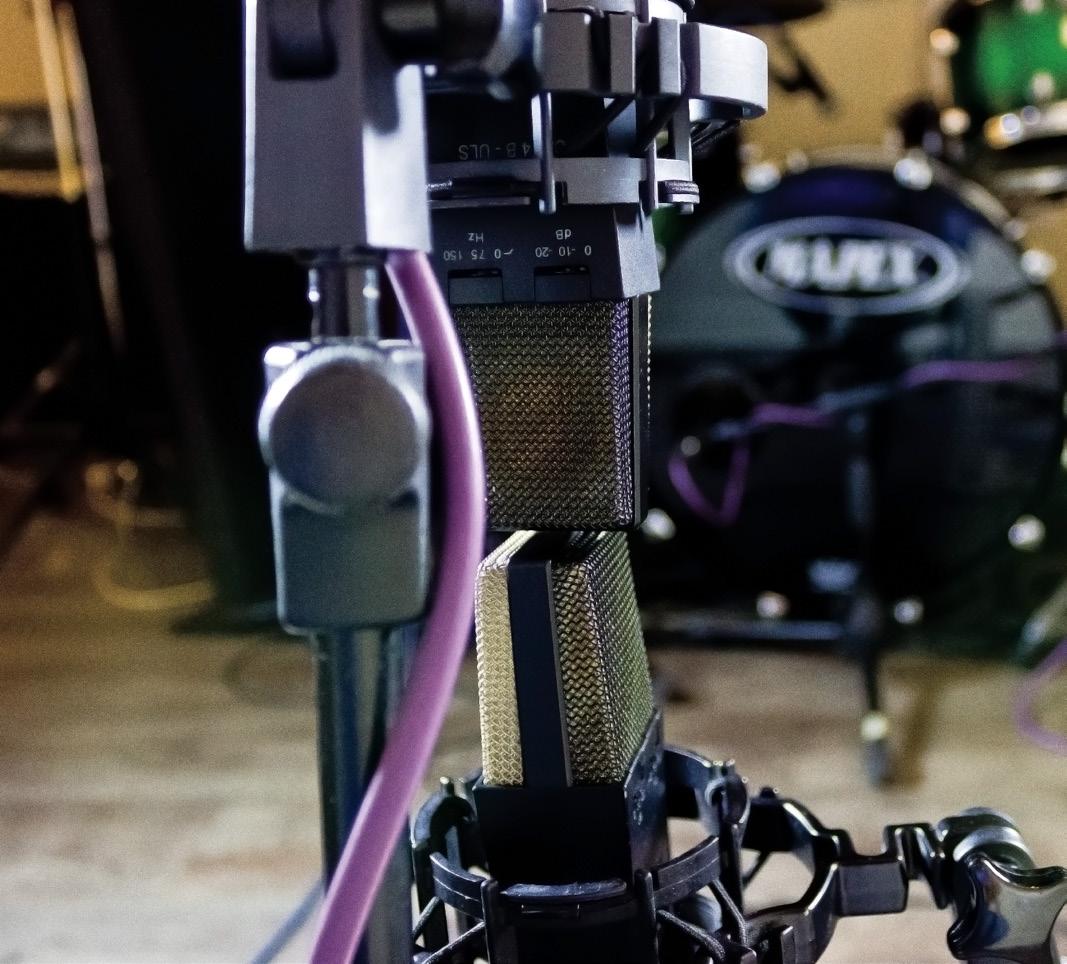
I’ll also discuss some tools that can help visualise and calculate the SRAs of different stereo arrays. As always, you can find the audio examples that

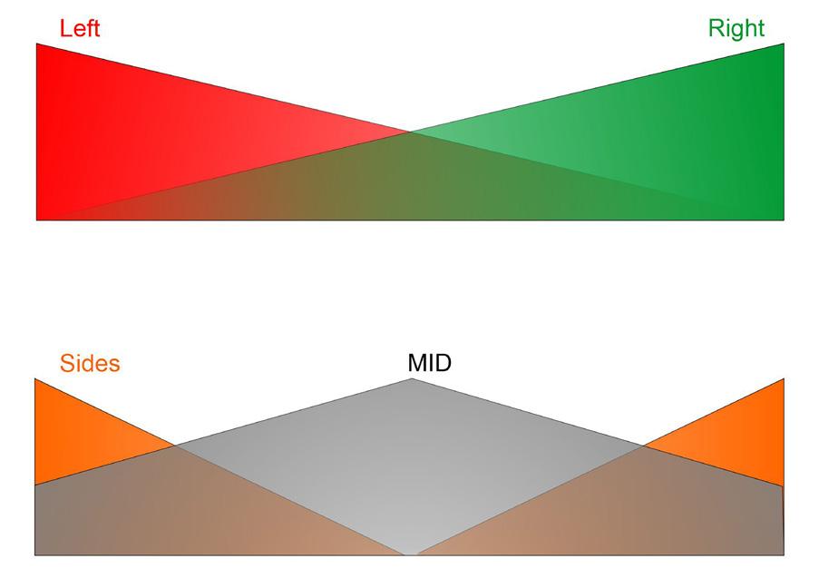
Diagram 1: M-S and L-R are both stereo formats, and carry exactly the same stereo information, but different parts of the signal are conveyed on each of the two channels.

accompany this series at https://sosm. ag/stereo-miking-demo-files

Mid-Sides

The term Mid-Sides seems to induce fear or confusion in many and, probably because the explanations often use equations, some seem to think it will be hard work! But Mid-Sides is really nothing more than the conventional left-right (L-R) stereo format viewed through a different lens, and in practice it’s very easy. L-R and M-S both carry exactly the same information, and are completely interchangeable through a simple ‘matrix’ process.

Diagram 1 illustrates how audio information is portrayed in each channel in both formats. In the L-R format (top), a fully-left sound source is carried only in the left (red) channel. But as soon as it starts to move towards the right, some left-channel information is also carried partly in the right (green) channel too. The further the source moves

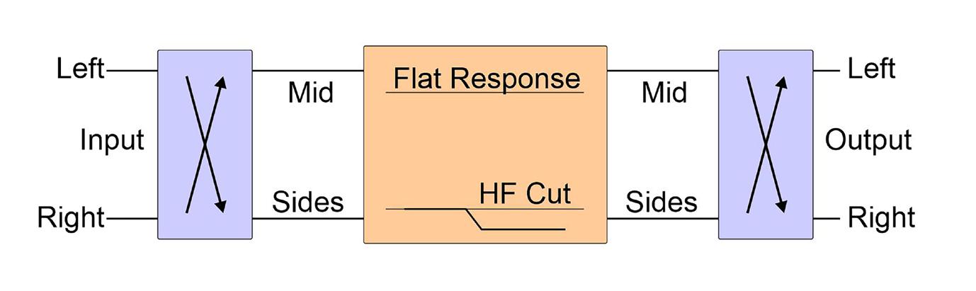
Diagram 2: EMI’s Stereosonic Shuffler employs a high shelf cut in the Sides channel to narrow the stereo image slightly at high frequencies.

right, the stronger it gets in the right channel. A central sound source is carried equally in the left and right channels, of course.

For the Mid-Sides format, the Mid channel carries everything, no matter where it is positioned in the stereo image. But a central sound is 6dB louder than if that sound was fully left or right, because the same signal exists in both channels (if you add two identical signals the result is 6dB louder). The Sides channel, as the name implies, is strongest for signals that exist only in one channel (whether left or right) at either side of the stereo image. The signal strength falls as the source moves towards the centre, and a central sound source is not carried in the Sides channel at all. And all of this behaviour is defined by two simple equations:

• Mid = Left + Right (the sum of both channels).

• Sides = Left - Right (the difference between channels).

Hopefully you can see that, since you’re adding the left and right, the Mid channel is exactly the same as a conventional mono sum. The Sides channel, on the other hand, essentially carries all the stereo-width ‘goodness’ that you lose when summing to mono — the wider a sound source in the stereo image, the stronger it will be in the Sides channel. Importantly, exactly the same sum and difference matrix processing converts the other way, too:

• Left = Mid + Sides (sum)

• Right = Mid - Sides (difference)

Consequently, whatever format you feed into an M-S matrix, the opposite format will appear at its output. L-R becomes M-S, and M-S becomes L-R; it’s the same process for both conversions. There’s a small but important caveat, though!

Imagine you want to convert L-R to M-S to adjust the stereo width, and then convert the narrowed/widened signal back to L-R (this is precisely what most stereo-width controls do in mixers). The first matrix outputs an M-S signal that we route into another matrix that outputs L-R. The stereo channels L and R that we start with become M (=L+R) and S (=L-R). Those M-S signals go into a second matrix to derive L and R again (L=M+S and R= M-S). But look what happens if we substitute those M and S terms in the second matrix for the Left and Right terms that we started out with:

• Left output = M+S = (L+R)+(L-R) = 2L

• Right output = M-S = (L+R)-(L-R) = 2R

As you can see in the rightmost part of those two equations, we now have twice as much output signal level as we started with. Put another way, the output of the second matrix is 6dB louder than the original signal. Sometimes that won’t matter, as it’s not difficult to adjust the signal level manually, but usually we need to preserve unity gain and headroom throughout a signal chain. A simple

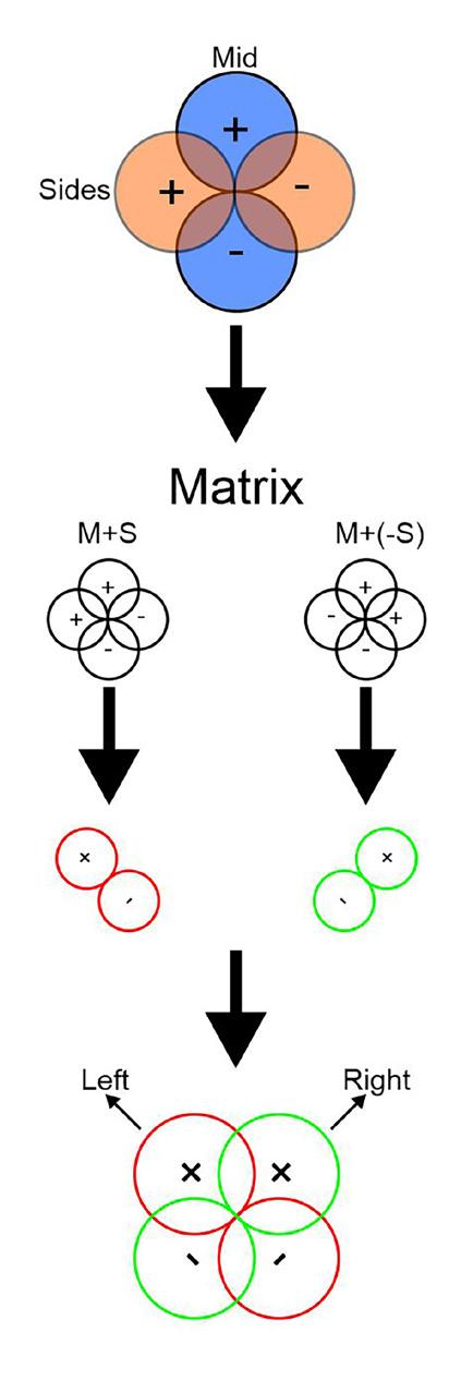
Diagram 3: A Blumlein Mid‑Sides array, matrixed to create a ‘virtual’ L‑R stereo array.

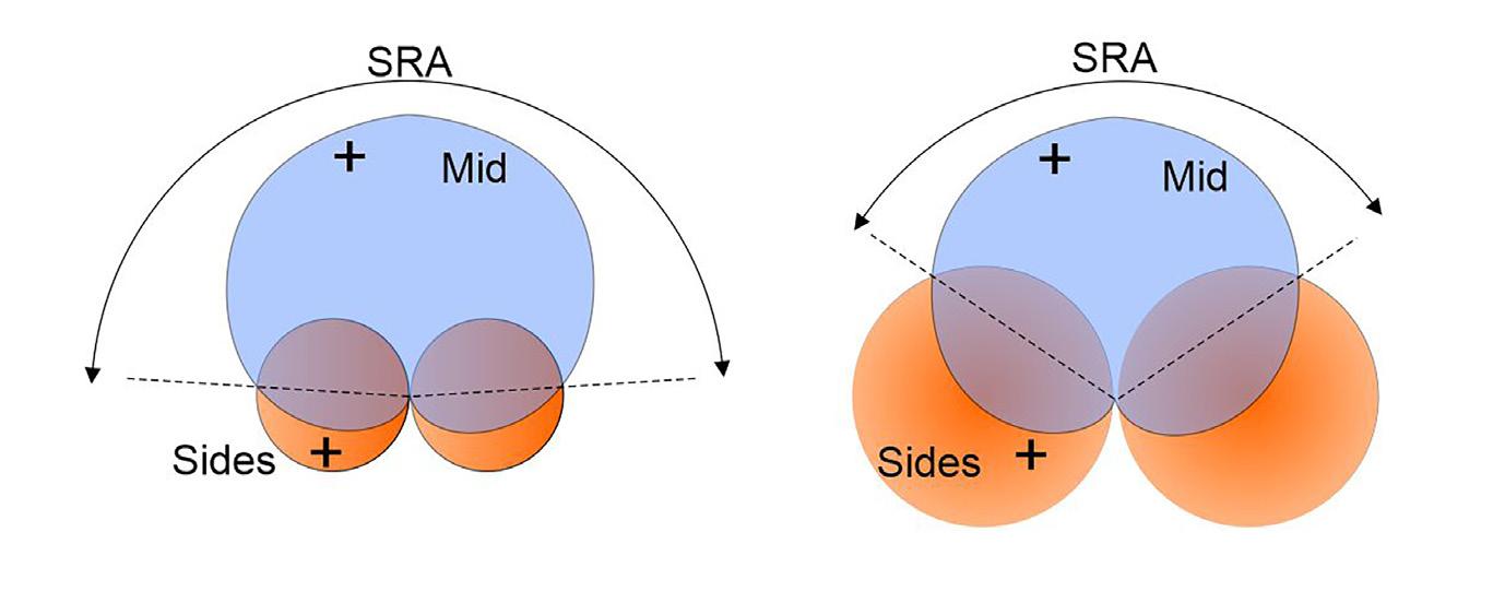
Diagram 4: Adjusting the relative sensitivity of the Sides microphone moves the points where the Mid and Sides polar patterns are equal in amplitude, which defines the edges of the SRA and thus the perceived stereo width of sources placed in front of the M-S array.

solution is widely (but not universally) adopted: each matrix is designed with 3dB attenuation at both its outputs. That way, when two matrix processes are combined, the overall signal maintains unity gain. If you notice a slight (3dB) loss in level when passing a signal through a single matrix, this will be why!

Practical Benefits Of Mid-Sides

OK, enough of all the maths! What is M-S actually useful for in practice? The main advantage of the M-S format is that varying the ratio of the Mid and Sides components adjusts the width of the stereo sound stage. With no Sides signal you’re left with pure mono. And as the Sides level is increased, the stereo width increases with it. Full (100 percent) width is when the Mid and Sides signals are exactly equal in level, and pushing the Sides level higher still creates an ‘out-of-phase’ effect, whereby sounds appear to come from ‘outside’ the speakers, but do so in a very unstable (and, often, arguably unpleasant) way.

The Mid and Sides signals can also be processed independently too, and a very powerful technique is to boost and/or cut the level of the Sides signal using an equaliser. This allows the stereo width to be adjusted in a frequency-selective way. For

example, rolling off the low end in the Sides leaves all the bass in the Mid channel only, so it’s all in the centre of the stereo image — this is a standard process for cutting vinyl records. Alternatively, using a high-shelf cut in the Sides channel narrows the stereo image slightly at high frequencies, and that’s exactly how EMI’s

Stereosonic Shuffler works (Diagram 2), as mentioned in chapter 3.

Mid-Sides Stereo Array

So far, I’ve discussed creating Mid-Sides signals from left-right stereo using a matrix process. But we can also capture M-S stereo signals directly at source,

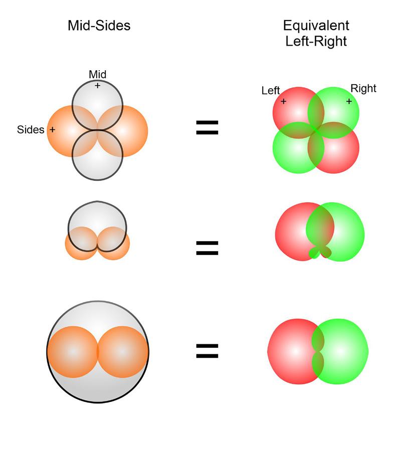
using a pair of microphones — an idea that Alan Blumlein came up with almost a century ago. Like conventional L R stereo, two microphones are required, and they must be mounted coincidently, such that they capture only amplitude differences between the two channels (ie. with no time of arrival differences).

The Mid signal can be captured using any desired polar pattern that ‘hears’ all the sound sources consistently, and provides a suitable perspective (in terms of the direct sound:reverberation ratio). Blumlein originally used a figure 8 ribbon mic for this technique, but hypercardioid, cardioid and even omnidirectional patterns are now common options, too. The Sides mic must reject sound sources at the middle of the stereo sound stage, so must have a polar pattern with a null facing forwards, but good pickup to either side. The perfect candidate for that role is obviously the figure 8 pattern, and the fact that its front and rear lobes inherently have opposite polarities is essential in making the maths work when decoding the M S signal to L R — those opposite polarities uniquely identify which sound sources are on the left or right.

Blumlein’s original M S array comprised a forward facing figure 8 mic for the Mid channel, and a sideways‑facing figure 8 mic for the Sides channel. Importantly, the face of the Sides mic facing left must have the same polarity as the front of the Mid microphone — in other words, the front of the mic should face left and its rear should face right. If it doesn’t, then the decoded stereo image will be left right reversed.

Diagram 3 illustrates how the different polarity lobes of the two figure 8 mics add and subtract through the decoder to create a virtual L R stereo mic array (which, in this case, happens to be a conventional Blumlein array).

A central sound source will only be ‘heard’ by the Mid mic because it’s precisely in the null of the Sides mic.

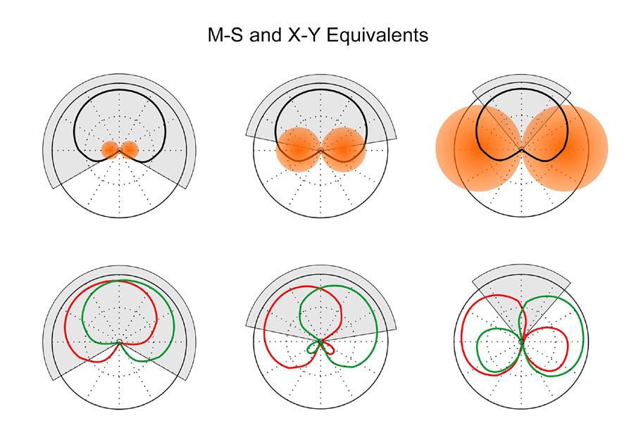
However, as that sound source moves off to the left, the Sides mic starts to pick it up and the Sides output level rises. At the same time, the Mid mic’s output level falls, as the source moves progressively off axis — there are pure amplitude differences between the Mid and Sides channels.

“The main advantage of the M-S format is that varying the ratio of the Mid and Sides components adjusts the width of the stereo sound stage.”

Use the M S equations I set out earlier, and you’ll find that when the sound exists only in one channel (eg. left only), it’s true that Mid=L and Sides=L. In other words, when a sound source is at the extreme edge of the array’s SRA — as far left or right as it can be — the Mid and Sides channels will have equal amplitudes. Put simply: M=S.

It follows that if the level of the signal captured by the Sides mic is

then increased at or after the preamp stage, then a central sound source won’t need to move as far left or right to generate the same output level in the Sides channel as it does in the Mid mic. In other words, the SRA is reduced! Conversely, if the Sides mic level is reduced, a central sound source needs to move much further out from the centre to generate the same signal level captured on the Mid mic, so the SRA increases.

Diagram 4 illustrates this using a cardioid Mid microphone with lines drawn from the coincident centre of both mics out to where the Sides and Mid patterns meet. These lines define the edges of the SRA and, as you can see, their position is dependent on the relative sensitivity of the Sides mic.

While it is certainly possible to decode the outputs from an M‑S array to record a normal left right stereo signal, the real benefit of the M S format is obtained by recording the M S signals directly, and decoding them to left right in post production, during the mix, when the appropriate stereo image width can be determined, or even adjusted dynamically.

Example 7 in the associated choir audio files was captured using an M S array and is recorded in

the M-S format. The output from a forward-facing cardioid mic (a Sennheiser MKH 40) is on channel 1, and a sideways figure-8 mic (MKH 30) on channel 2. When these tracks are loaded into a stereo track in a DAW, the resulting raw material will sound noticeably left-dominant, because the Mid mic in the left channel is facing the choir whereas the Sides mic in the right channel isn’t. Inserting an M-S decoder plug-in into the stereo track will decode the signal to normal left-right stereo, and produce

M-S Matrix Technologies

a stereo image similar to that from the coincident hypercardioids used in Example 5. If the level of the Sides channel is adjusted (whether using the decoder plug-in’s controls, or the right channel’s input gain), the stereo image width can be varied all the way from mono (phantom centre) up to ‘outside the speakers’.

Equivalences

When a figure-8 mic is employed for the Mid channel in an M-S array, the equivalent left and right

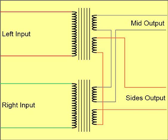
Converting from L-R to M-S (or vice versa) can be achieved in a variety of ways, but originally it was performed passively, using transformers. Each channel used a transformer with a single input (primary) winding and two secondary output windings, typically with a ratio of 1.4:1:1. Each of the matrix outputs are derived by wiring a secondary in each transformer in series, either in the same polarity (for the sum output), or in opposite polarities (for the difference output), as shown in Diagram 8. However, this is a bulky and expensive solution, and analogue matrix systems today typically use op-amps to add and subtract the input signals (Diagram 8b), usually achieving better frequency and phase responses, too.

The same conversion processes can also be achieved

‘virtual’ mics are a classic Blumlein array, as already illustrated. But if an omnidirectional mic is used instead, the decoded virtual mics turn out as back-to-back cardioids, with a mutual angle of 180 degrees — a handy format for capturing ambient atmospheres. More commonly, though, cardioid or hypercardioid patterns are employed for the Mid mic, creating virtual left-right mics which are a little more directional than the real Mid mic’s pattern, and with a mutual angle

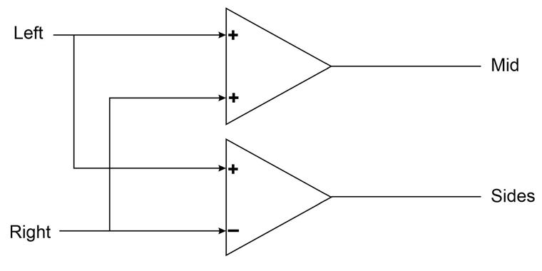
Diagram 8a (left): A traditional M-S matrix, using a transformer for each channel with a single primary coil and two secondaries. Diagram 8b (above): The electronic equivalent.

by routing signals around an analogue console using channel pan pots and polarity inversions to add and subtract the Mid and Sides signals en route to the left-right stereo bus outputs (remembering that mixing two signals together when one is polarity-inverted is mathematically the

same as subtracting one signal from another). There’s a more detailed explanation of these arrangements in the ‘Decoding M-S Mic Arrays In A Mixing Console’ box, and I’ve included a couple of examples on the SOS website.

The same console signal routing concepts could be

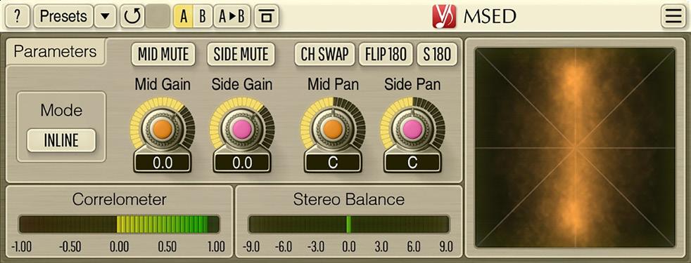
employed within the virtual mixer of a DAW, of course, but why would you when it’s so much easier to use an M-S decoder plug-in? Most DAWs include this functionality but, if not, Voxengo’s MSED is free, very easy to use, includes useful stereo metering, and is highly recommended.

determined by the ratio of Mid and Sides levels through the decoder (see Diagrams 5a and 5b).

In addition to being able to adjust the SRA during or after the recording, another important advantage of the M-S array is that central sound sources are always directly on-axis to the Mid

microphone. The relevance of this is that, as already mentioned, most directional microphones get more directional with increasing frequency. With conventional left-right coincident arrays, a central source is always inherently off-axis to both mics, and therefore potentially coloured due to the imperfect polar

Decoding M-S Mic Arrays In A Mixing Console

The key to decoding Mid-Sides signals through an analogue mixing console is to keep in mind the core equations: Left = M+S and Right = M-S. The act of mixing signals together is the equivalent of adding them, and while subtraction isn’t a standard feature of a mixer, a little algebraic rearrangement gives us: Right = M+(-S). In practical terms, that minus sign simply indicates a polarity-inverted signal — in other words, we simply need to mix a polarity-inverted Sides signal with the Mid.

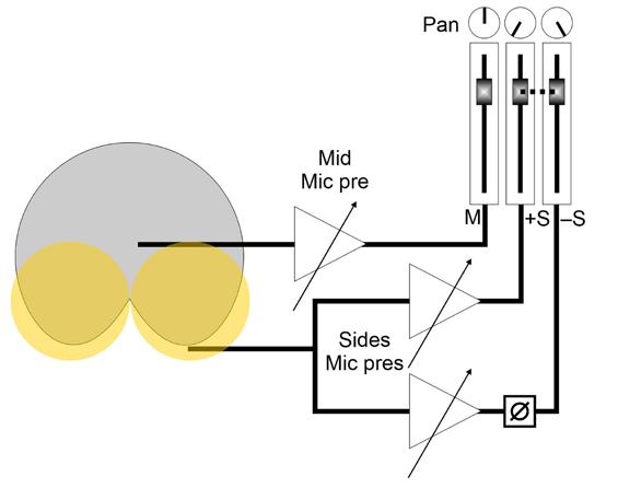
With all this in mind, the simplest console setup to decode an M-S mic array to the L-R stereo bus output is to start by setting the Mid channel’s pan to the centre, thus ensuring that it contributes equally to both the left and right outputs. The Sides signal feeds the left output, where it is summed with the Mid — so the Sides channel must be panned fully left. We also need the polarity-inverted Sides signal summed to the Mid at the right output. The classic way to achieve this is to duplicate the Sides channel, put this duplicate on a third channel whose polarity-inversion (erroneously called ‘phase’ on many mixers) button is engaged, and pan it hard-right. The faders of both the original and duplicated Sides channel need to be linked so that both are moved together when adjusting the stereo width.

This arrangement (Diagram 10) works perfectly well, especially with line-level sources. But if decoding an M-S mic array, splitting the Sides mic across two channels isn’t the best idea because it halves the input impedance seen by the mic. The arrangement also occupies three adjacent mixer channels and relies on perfect tracking of the two Sides faders. A better-engineered solution is to connect the Mid and Sides mic outputs to a pair of mono channels in the normal way, with the Mid channel panned to the centre, and the Sides channel panned hard-left, as before. To generate the inverted Sides signal,

Diagram 10: The classic way of accommodating a Mid-Sides array on a mixer, with a splitter allowing the Sides mic to feed two channels. It works, but is not ideal!

pattern frequency response. This is especially true where very wide mutual angles or highly directional polar patterns are employed. Using the M-S format guarantees that a central source — which is usually the most important element — is captured with the mic’s ideal on-axis frequency response.

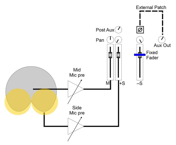
use a post-fader aux send and connect the corresponding aux master output to a spare channel somewhere out of the way on the desk. That channel should have its polarity-inversion button engaged and be hard-panned to the right, as before, but its fader should be set to unity and taped down so it can’t move!

The next stage is simply to match the aux send signal with the Sides channel’s level so that the +S and -S contributions to the left and right outputs are perfectly balanced. To achieve that, set the Sides channel’s aux send and the corresponding aux master to their unity reference levels. Open the Sides channel fader to 0dB, and switch the console monitoring to mono. Now adjust the aux return (-S) channel’s gain for the deepest possible null, indicating a perfect balance of the +S and -S contributions to the stereo L-R mix. Once set, you will not need to touch the aux controls of the -S channel gains again — but don’t forget to deselect the mono monitoring!

This alternative arrangement (Diagram 11) makes it easier to adjust the Sides level without having to worry about ganged faders, and it also presents both mics in the array with standard mic input impedances. In situations where you are using more than one M-S array, this arrangement also saves channels as each new array just needs two (one for Mid and another for Sides). The aux return channel already set up will also generate the -S contributions from the second array! Just fine-tune the post-fader aux send level from the second Sides input while listening for a mono null.

Diagram 11: A better M-S approach on a console is to connect the Sides mic’s preamp to one console channel, and use a unity-gain post-fader aux send to mult the signal to a unity-gain channel elsewhere on the console.

Chapter 5 Spaced Arrays

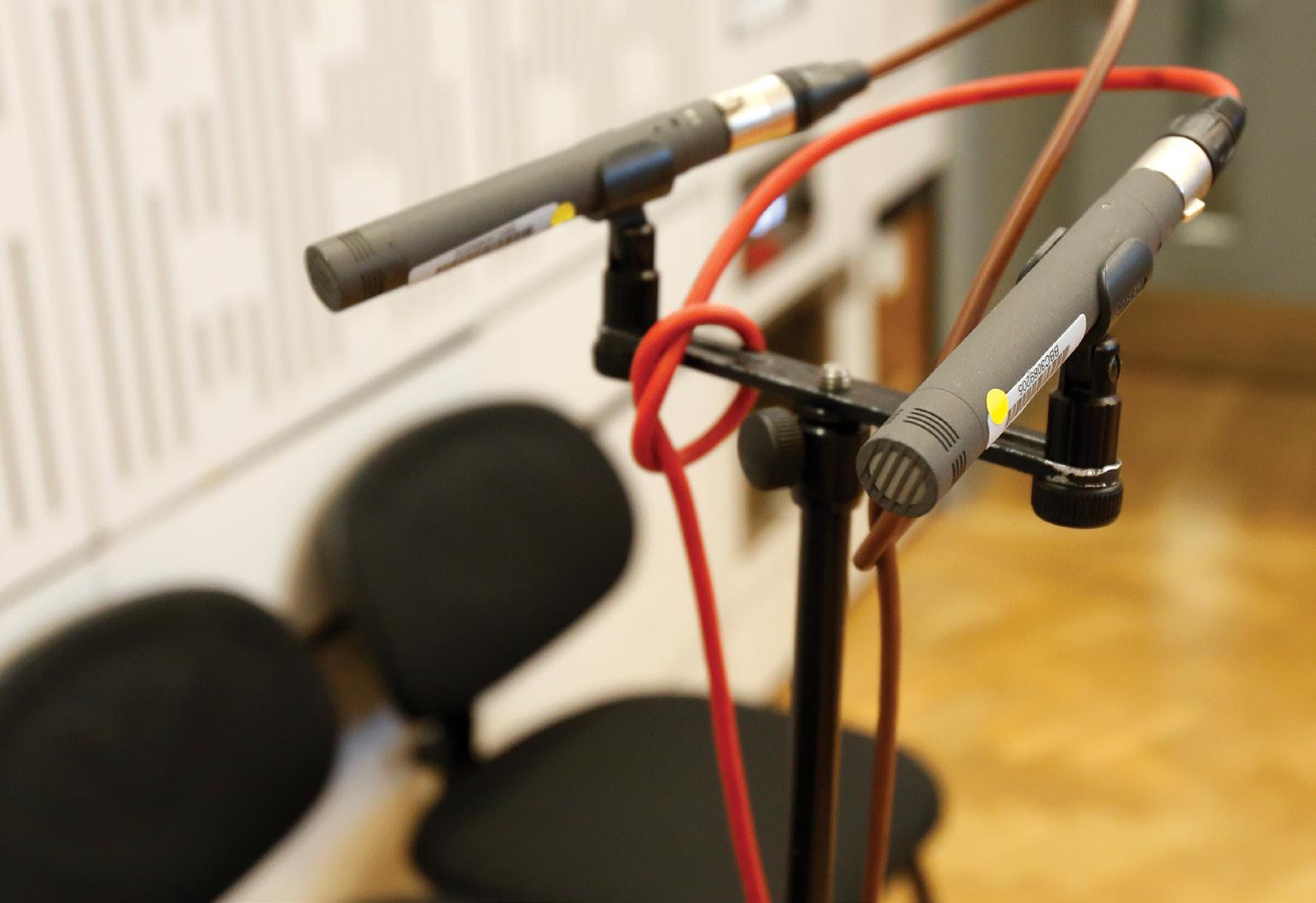
Building on concepts explored in previous chapters, it’s time to consider the relative pros and cons of coincident and spaced arrays...

Previously in this book I focused on a range of coincident microphone techniques, and you’ll recall that with all such techniques, perceived position on playback depends entirely on level difference in the two channels. This time, we turn our attention to spaced stereo arrays, which introduce time-of-arrival differences between the two microphones. These give an entirely different sense of stereo imaging — less precise and more diffuse — but it’s often also subjectively appealing, and there can be benefits as I’ll explain below.

Precision Position

First, let’s pick up on that point about ‘precision’. With coincident

arrays, equal volumes in each channel create a ‘phantom’ central image source in the speakers, and introducing a level offset between the channels moves the sound source towards the louder channel’s speaker. It’s not equal for all frequencies, though.

For mid and high frequencies, which tend to be portrayed wider than intended when auditioned over stereo loudspeakers, an offset of around 4dB places the sound about a quarter of the way out towards one speaker. 8dB is half-way, 12dB is three-quarters, and 16dB puts the source firmly in one speaker (see Diagram 1).

These are only rough guide numbers — different listeners and different monitoring environments

might need smaller or larger offsets to achieve the same perceived image positioning. But slightly larger offsets are typically needed to match positions for the lower frequencies. It’s why EMI developed the Stereosonic Shuffling correction process I described back in chapter 3. (There are other issues that affect the precision of stereo imaging over speakers, and various remedies, but I’ll save that for later!)

Coincident mic arrays aren’t the only means of creating the impression of different spatial positions, though. As Dr Fletcher discovered with his ‘curtain of sound’ experiments, reproducing small inter-channel timing differences also works — though arguably with less well-defined image locations.

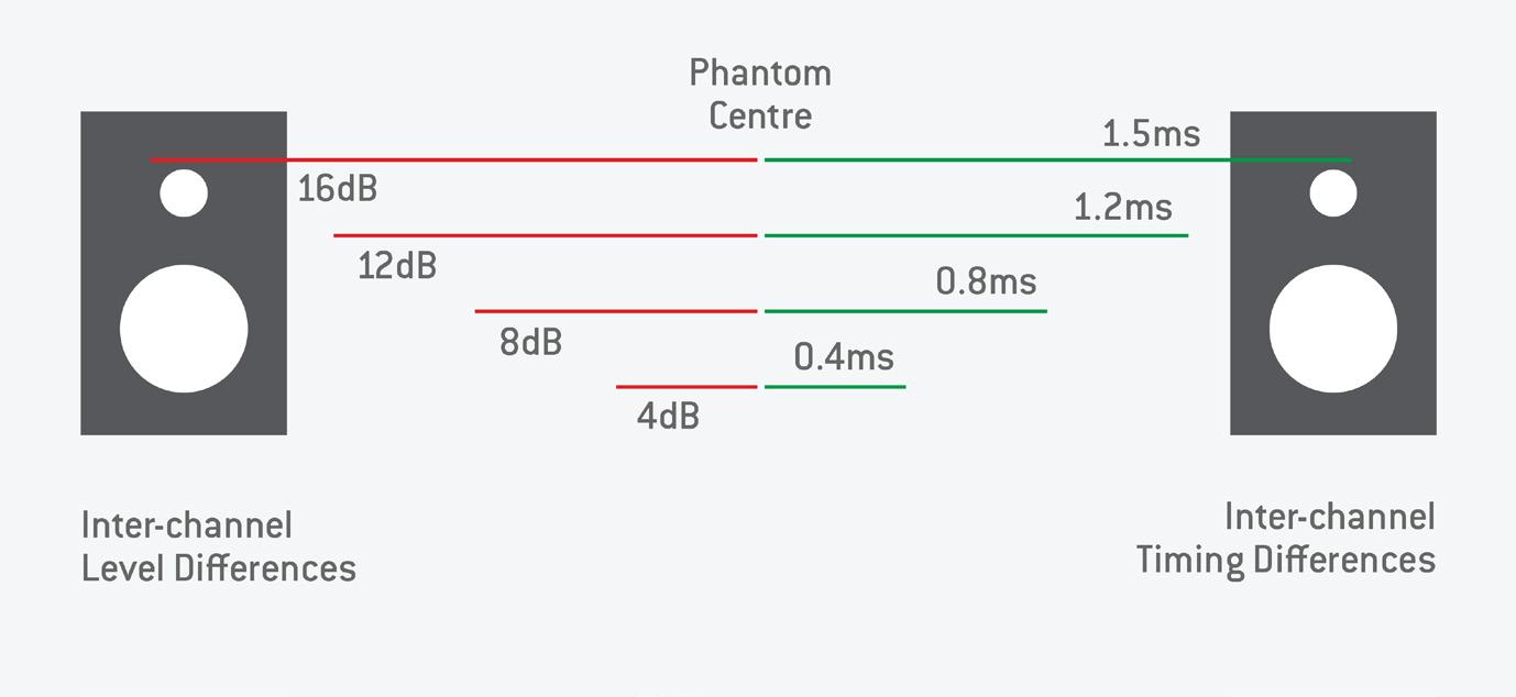
Remember, the ear/brain system uses inter-aural timing differences to help locate sound sources around us, and for a source located 90 degrees to one side, the difference in arrival times for a sound at each ear is about 0.67 milliseconds. Yet, if we introduce that kind of time delay between channels replayed over stereo loudspeakers, the sound source will be perceived as being barely half-way towards the earlier

loudspeaker — this is because sound is coming from both loudspeakers, each introducing their own time delays for sound arriving at each ear. Essentially, it’s an unnatural and confusing situation, as far as the ears/brain are concerned. We can still create the impression of a sound source being fully in one loudspeaker, but the time offset between channels actually needs to be around 1.5ms (again, see Diagram 1).

Subjective Differences: Audio Examples

In the main text, I said that spaced-omni microphones portray stereo positioning in a radically different way from coincident mics, and that most listeners perceive spaced-omni recordings as creating a much less precise sense of image positioning. To relate the differences to another artform, if the coincident format is likened to a fine-art oil painting, the spaced-omni approach is perhaps more reminiscent of an impressionist watercolour — while a bit blurry and unfocused, the information is there, and sometimes that sound character is precisely what is desired. Personally, I think the spaced-omni approach suits orchestral music in particular, as it gives an homogenous, spacious and luxurious kind of sound; it doesn’t generate lots of potentially distracting detail.

A second benefit associated with the A-B technique is that omni mics usually have a much more extended low end than typical directional microphones, as well as negligible phase-shift and a more natural and neutral sound character. Consequently, the spaced-omni approach is often favoured in situations where those features are beneficial to the material being recorded, over and above the format’s stereo imaging characteristics.

As well as understanding the theoretical difference, it’s good to experience the differences in sound for yourself. So, if you

So, if we’re to utilise inter-channel timing differences to create the illusion of sound source positions between stereo loudspeakers, how can we arrange a pair of microphones to capture only suitable inter-channel timing differences that relate proportionally to the real sound source positions? It’s probably fairly obvious that to capture time-of-arrival differences between the two channels, we’ll need to space the mics apart

get a chance, check out audio examples 7, 8, 11 and 12 in the media files associated with this series (on the SOS website: https://sosm.ag/stereo-miking-demo-files). These illustrate the stereo imaging characteristics of spaced-omnidirectional microphones versus coincident arrays. I recorded two basic A-B pairs in my ad hoc session with the Teme Valley South Churches Choir (TVSCC). Track 11 (OCCO Omnis) was captured with a pair of Sennheiser MKH 20 omni mics, spaced at 69cm to give an SRA of 96 degrees, at a medium distance from the choir. You can compare the stereo imaging with the (decoded) Mid-Sides array (track 7), mounted in the same location and using the same family of microphones (MKH 30/40). When decoding the Mid-Sides array, adjust the Sides channel’s level to achieve a similar overall stereo width as the OCCO omnis — about +2dB if using the Voxengo plug-in. Track 12 (Wide Omnis) uses the same Sennheiser MKH 20 omni microphones, but spaced much wider (83cm) for an SRA of 75 degrees. These mics were placed further from the choir, alongside the Neumann SM 69 set up as coincident figure-8s (track 1). Again, these two mic arrays have the same nominal SRA, so their imaging characteristics can be compared directly, albeit with a more distant perspective than the previous examples.

Diagram

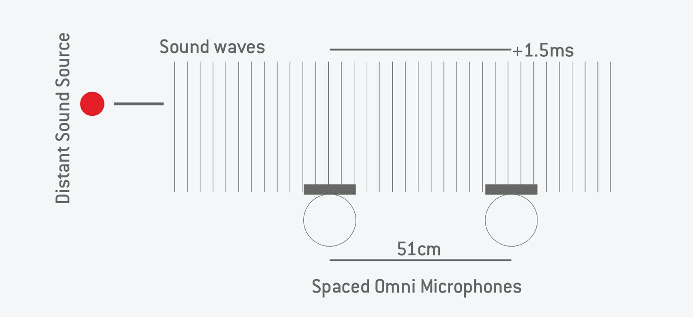
If the distance between mics is less than 51ms, no sound will appear to be ‘fully panned’.

by a small distance: sound from a central source will arrive at both mics at the same time (giving a central phantom sound image), but sound from a source located to the left will reach the left microphone slightly before the right one, resulting in a small time difference between the channels.

With the two microphones spaced apart, the inverse-square law of sound propagation — sound energy decreases with distance from the source — means that the more distant mic will also always receive a slightly lower sound level than the closer mic, so a small level difference between channels will be captured too. However, if the mics are reasonably far away from the sources, but not too far apart from each other, any channel level difference will be insignificant in terms of sound image location information. Moreover, if we use omnidirectional microphones, the relative angle of sound incidence won’t affect the sound level either...

Spaced Omnis

So, we have a pair of omnidirectional microphones spaced apart specifically to capture time-of-arrival

differences — a technique generally referred to as ‘spaced omnis’ or A-B stereo (in contrast to the coincident or X-Y stereo technique). As an aside, it’s worth noting that Alan Blumlein also experimented with spaced omnidirectional mics in the 1930s, coming up with an arrangement most know today as the Jecklin disc; I’ll discuss that concept in detail in chapter 9. If two omnidirectional mics are mounted coincidentally, there can be no level or timing differences between the signals they capture. Whatever the sound source’s position relative to the mics, identical signals in both channels will create a phantom central image over the stereo loudspeakers. If the mics are gradually moved apart, though, sound from a source located to one side of centre-stage will reach the closer mic slightly before the more distant mic, resulting in a small inter-channel timing difference.

So, what kind of mic spacing do we need to generate an inter-channel timing difference sufficient to place the sound fully wide in one loudspeaker? Consider a sound source, located at 90 degrees to the microphones

(ie. fully left), that we want to perceive fully in the left-hand speaker. As suggested above, the sound waves must arrive at the left-hand microphone 1.5ms before passing across to the right-hand microphone. Sound travels around 34cm per millisecond, so achieving that delay requires the mics to be spaced 51cm (34 x 1.5) apart, as in Diagram 2.

Put the mic capsules closer together than 51cm, then, and it will always be impossible to generate a timing difference between channels as large as 1.5ms, whatever the source position — the image width on loudspeakers will always be narrowed, and collapses to a phantom centre as the capsules approach one another. Conversely, if the capsules are moved further apart, a sound source would need to move a smaller distance from the centre line to generate the 1.5ms difference.

This gives us a very practical way of controlling the Stereo Recording Angle (SRA) from spaced-omni microphones: increasing the capsule spacing reduces the SRA. We’ve seen that a capsule spacing of 51cm gives an SRA of 180 degrees, while increasing the

spacing to 73cm reduces the SRA to about 90 degrees. Inevitably, if the capsules are moved too far apart, the channel timing differences generated by off-centre sound sources can exceed 1.5ms. That breaks the stereo system — instead of a continuous spread of sound between the two loudspeakers, we perceive ‘puddles’ of sound localised at each speaker, with a gaping ‘hole’ in the middle of the sound stage. This ‘hole-in-the-middle’ effect was quite common in early commercial stereo recordings, partly by design, as record labels tried to emphasise the benefits of two-channel recordings: “Completely different sounds from your two loudspeakers — so much better than mono!” Some labels cured this hole-in-the-middle problem by adding a third, central, omni mic... Again, I’ll explore that in a later chapter.

SRA Rules

In chapter 3, I defined Rule 1, for fine-tuning the SRA of a coincident array by adjusting the mutual angle. We can now add a second rule for the capsule spacing in spaced arrays:

• Rule 1: Reducing the Mutual Angle (MA) increases the Stereo Recording Angle (SRA).

• Rule 2: Reducing the Capsule Spacing (CS) increases the SRA.

In both cases, reducing the separation between the microphone capsules increases the SRA, and increasing the separation decreases the SRA. This makes sense if you think about it because if the capsules are closer or pointing in similar directions, a sound source has to move further out to create a sufficient level or time difference between the two channels. With coincident X-Y arrays, the useful range of mutual angles between capsules is typically from about 75 to 120 degrees, with 90

degrees as the nominal sweet spot, although the actual SRA also depends heavily on the chosen polar pattern of the mics. For an A-B or spaced-omni array, the useful capsule spacing ranges from 51cm to about 1.5 metres, corresponding to SRAs of 180 to about 40 degrees, respectively. The sweet spot is usually somewhere around 66cm (SRA = 100 degrees) in my experience, but the required SRA (and thus spacing) depends mainly

(ITDs) at the ears — these being critical in our perception of spatial positioning. Listening through headphones inherently removes the ‘crosstalk’ between source loudspeakers and ears, since each ear can only hear the channel feeding that earpiece. Consequently, when wearing headphones only the ILD and ITD information embedded within the two-channel stereo signal is available to the brain to try and work out source locations.

“ Spaced-omni recordings generally sound much more natural than coincident ones when auditioned on headphones.”

on how far back from the source the mic array must be to achieve the appropriate perspective or acoustic ambience. In the next chapter, I’ll introduce two fabulous software tools for visualising and calculating the SRAs for most coincident microphone arrays — and of course, both can also demonstrate and calculate the SRAs for spaced-omni microphone arrays too. And if you want to compare the effect of the different approaches, see the ‘Subjective Differences: Audio Examples’ box on the previous page.

Speaker & Headphone Listening

Of course, although stereo recording was originally conceived and developed for reproduction over loudspeakers, that’s not the way a large number of people listen to their music today. Headphones (and earbuds) have become very popular, but they present sound to the ears in a very different way. When listening to loudspeakers both ears hear both loudspeakers and that inherently results in both inter-aural level differences (ILDs) and inter-aural timing differences

The Intensity Stereo format, using coincident mics, explicitly excludes all timing differences between the channels, so there is no ITD information for the brain to decode. This is a very unnatural situation, impossible in real life, and the result is that most people’s brains deduce a solution where the sound sources exist inside the head, spread along a line between the ears, rather than outside it. In contrast, the spaced microphone technique does capture time-of-arrival information between the channels — albeit with very large ITDs — and that is passed directly to the listeners ears when wearing headphones or earbuds. Consequently, spaced-omni recordings generally sound much more natural than coincident ones when auditioned on headphones, often with the impression of sound sources outside the head, and the imaging tends to be more precise and less vague than if auditioned over loudspeakers. Again, you can try this for yourself using the same tracks linked to in the box — but this time listen over headphones and compare the results with the stereo imaging over loudspeakers.

Various software tools and meters can help you set up and refine your stereo arrays with precision.

Chapter 6

Useful Software Tools

When rigging any stereo microphone array, it should be clear by now that two key parameters are paramount: the sound-stage perspective (the direct/reverberation balance), and the width of the sound sources across the stereo image. The first is dependent on the room’s acoustics, and the mic array

needs to be moved closer or further away from the sound sources to achieve the preferred perspective. Once that position is known, the stereo recording angle that’s needed in order to encompass all the sound sources can be assessed. But how, then, can a specific mic array setup be found to match that SRA requirement?

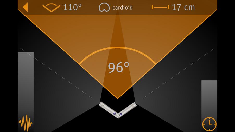
When it comes to working out how to achieve a specific SRA, or trying to visualise how changing polar patterns and mutual angles interact, there are a couple of interactive tools that I find particularly helpful (though note that neither have options for M-S arrays). When working on location, I mostly use the Neumann Recording Tools app (Diagram 1), which I reviewed in the August 2018 issue of Sound On Sound: www.soundonsound.com/reviews/ neumann-recording-tools. It was free and available for both Android and iOS. Sadly, though, while it still works on my phone, it’s no longer available, due to incompatibility with recent OS releases. Still, I’ve been corresponding with Neumann about this, and have hopes that they will eventually be able to update and re-release it, so I think it’s worth describing its benefits here.

This app is actually two apps in one, with one section offering a comprehensive gain and

The BBC’s Twin‑Twin Peak Programme Meter (PPM)

The BBC, since its inception, have always used the PPM as the standard level indicator, with its unique 1-7 scale. When stereo was being introduced at the BBC in the 1960s, the corporation developed a unique dual-concentric twin-needle meter movement with a British manufacturer Ernest Turner (and later manufactured by Sifam).

These were mechanically identical and only differed in the colours of their two needles. The Type 74B has red (left) and green (right) needles to indicate the left and right channel levels against a black background with the standard white scale numbered from 1 to 7. The red/green colour allocation is the same as aircraft and ship navigation lights, and the red needle is always in front of the green.

The Type 74A has white and (originally) all-yellow needles to show the sum (Mid) and difference (Sides) signals, respectively (white at the front). However, it was found that the yellow needle tended to fade over the years, becoming whiter, while the white needle tended to oxidise towards a yellow hue… which could become quite confusing! Consequently, around the 1980s the yellow needle was replaced with a black one which had a fluorescent orange tip to avoid any confusion! (The zplane PPMulator XL plug-in retains the traditional all-yellow ‘S’ needle).

A typical BBC console installation employed a pair of these twin PPMs with a 74B on the left showing the left/right signals, and a 74A on the right showing the sum/difference signals, as shown in Diagram 3. When the BBC first started broadcasting in stereo, the content was mainly classical music, and it was found that the mono sum of a typical stereo recording was about 3dB louder than either the left or right channels because they were largely decorrelated. Consequently, it was decided that the circuitry driving the M-S meter would attenuate the outputs to both needles by 3dB, such that the left/right and sum needles all showed roughly equivalent peak levels. This configuration later became known as M3.

However, commercial broadcasting worked mostly with centre-panned speech and pop music mixed with all the louder instruments and vocals panned centrally. This kind of material has strong correlation between the two channels, resulting in the Mid signal being around 6dB higher than either channel individually. As a result, they decided to implement 6dB attenuation to the M and S meter signals — a configuration now known as M6 — giving roughly equal peak levels on the left, right and sum meters. This alignment also makes calibration with reference tones easier as all three needles sit exactly on PPM 4. The BBC converted its M-S meters to the M6 configuration in the 1990s, and

Other Stereo Metering Tools

Although the final arbiter of good stereo imaging must be the ears, there are several metering tools which I find very helpful, both for confirming what I’m hearing by providing a reliable qualitative reference point (especially when working on location or with unfamiliar monitoring setups), and for highlighting any imaging issues my ears may have missed! As a BBC-trained audio engineer I was taught to appreciate the stereo information presented so cleverly on the uniquely British ‘twin-twin PPMs’. If you’re interested in learning more about the BBC twin-twin PPM system, check out the other box in this article. While hardware twin-twin PPM units become available on the various online marketplaces from time to time, I can also recommend an excellent plug-in emulation called PPMulator XL from zplane (https://products.zplane.de/legacy-products) but be quick — zplane are discontinuing it soon!

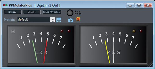
zlane’s PPMulator XL plug-in (Diagram 3) can be configured for either M3 or M6 modes. I’d argue that the M3 option is better for classical or other wide stereo music material, while M6 is better for mono speech and popular music.

In use, the benefits of the twin-twin PPM display are many. Firstly, it’s very easy on the eye, and the angles of the needles immediately convey the signal level without having to refer to the scale. Secondly, the relative level balance between channels is instantly apparent from the angle between the red and green needles (which remains consistent at all volumes). There’s 4dB between each pair of scale numbers on a BBC PPM, so an offset of one number (eg. one needle peaking to 4 and the other to 5) indicates a sound source with a 4dB offset, which would position it roughly a quarter of the way across the sound stage from the centre. An offset of two scale marks (8dB difference) indicates a sound source roughly halfway to the loudspeaker... and so on.

In a similar way, the angle between the M and S needles indicates the stereo width. A centre-panned signal leaves the S needle on the bottom stop, but as the stereo width increases the gap between M and S narrows. When the M needle lies directly over the S needle the stereo signal has full width (or a mono source has been panned fully to one side). If the S needle rises above M then there are strong out-of-phase elements in the mix, potentially reducing mono compatibility (the equivalent of a reading between 0 and -1 on a standard phase correlation meter).

I still use a hardware twin-twin PPM on my mastering console in the studio and rely on it all the time as I find it much more intuitive and easier on the eye than bar-graph meters in the DAW. When recording with a laptop on location I regularly use the PPMulator XL plug-in — such is the wealth and value of the information that can be gleaned in an instant from this marvellous vintage stereo metering system.

Phase Correlation Meter: Outside of the BBC, the recording industry historically relied on the humble Phase Correlation Meter, typically used alongside left and right VU meters. The classic phase correlation meter usually has the right half of the scale coloured green and the left half red (sometimes with a yellow region across the centre). More modern systems are typically configured as a bar-graph meter, but either way the display shows the instantaneous phase difference between the left and right channels. The scale ranges from -1 (180 degrees) at the left or bottom of the red region, through 0 (90 degrees) at the centre, up to +1 (0 degrees) at the right or top of the green section (see Diagram 4). So, when the two channels are identical (eg. a centre-panned signal) the display sits solidly at +1 (0 degrees), and if the two channels have opposite [continued overleaf]

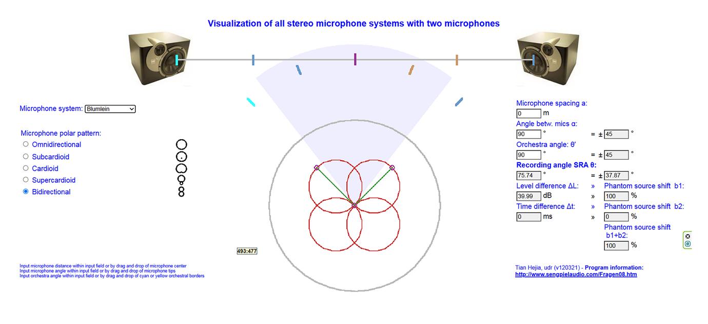
signal level calculator for the entire recording chain. The second section is the part that’s relevant here — it’s an SRA calculator, allowing the user to select and adjust polar patterns, mutual angle, and capsule spacing, with the resulting SRA illustrated graphically, along with indications of the relative proportions of inter-channel level and timing differences. This app is both accurate and easy to use and, by holding the phone horizontally you can squint across the top of the screen to see if the SRA is adequate for the sound sources in front of the mics.

A second option that I’d recommend, particularly in the absence of the Neumann app, is a web page on the very comprehensive Sengpiel audio tools website (https://sengpielaudio.com/ HejiaE.htm). Called ‘Visualisation of all Stereo Microphone Systems with Two Microphones’, it is similar to the Neumann app, but has some useful additional features (see Diagram 2). For a start, it has presets for a number of well-established stereo mic arrays, which are selectable from a drop-down box on the left-hand side. Alternatively, polar pattern, mutual angle and capsule spacing options can be entered manually.

The graphic display shows the selected mic polar patterns in red, and their mutual angle can be adjusted by dragging one of the circles at the top edges of the individual patterns (or by entering a value in the corresponding data box to the right). Similarly, the

the outer bars or entering a value in the Orchestra Angle data box. These virtual sources are mapped between the loudspeakers above, indicating any spatial distortion generated by the particular mic array parameters. The SRA for the displayed mic array is given in another data box on

“These applications help develop a mental picture of the way adjustments to the physical parameters of a stereo mic array impact the stereo recording angle.”

capsule spacing can be adjusted by dragging the circle in the centre of the mic array (or by entering a value in the data box). The grey outline surrounding the red mics is the equivalent polar pattern if the two channels are summed to mono (so equivalent to the Mid mic), while the blue-grey wedge indicates the SRA for the combination of selected microphone array parameters.

Five coloured bars arced across the SRA region represent notional (orchestral) sound sources in front of the mics, and their spread angle can be adjusted either by dragging

the right, along with the maximum inter-channel amplitude and timing differences, and their contributions to the overall imaging positions. I find it highly instructive to experiment with both of these applications to help develop a mental picture of the way adjustments to the physical parameters of a stereo mic array impact the stereo recording angle. With practice, adjusting mic array parameters will become instinctive if you need to increase or decrease the mutual angle to compensate for moving the mic closer or further away, for example.

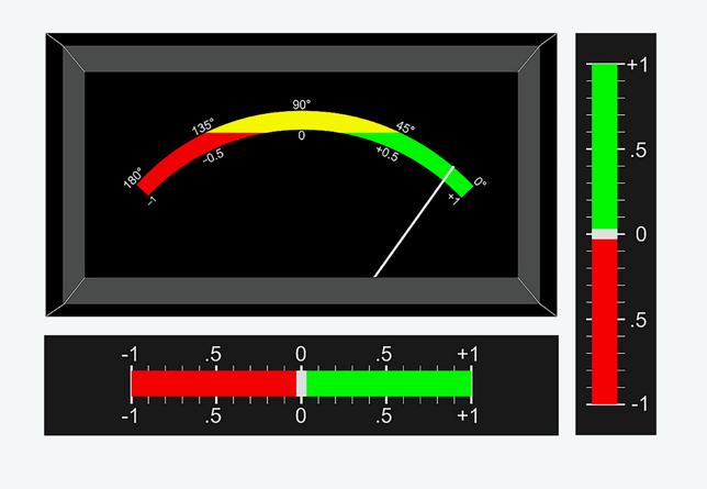
polarities (ie. fully out of phase) it will indicate -1 (180 degrees). A full-width stereo signal typically registers around 0 (90 degrees), so the aim for a good, wide stereo mix is to get the meter approaching as close to zero as possible, ideally from the positive (green) side!

With most commercial stereo material the meter typically sits within the green, positive section most of the time, and usually fairly close to the zero, although if the music has strong central components (vocals, bass, kick/snare) the meter will move closer to the +1 end. If it’s hovering around the zero but dips briefly into the red or negative section there’s usually nothing to worry about — it’s just showing instantaneous phase excursions over 90 degrees.

However, if the meter remains consistently below zero, in the red area, that indicates a potential problem with mono compatibility due to strong out-of-phase components in the mix (such as a stereo chorus effect or overly wide reverb, perhaps). So, although very simple, the phase correlation meter provides a very helpful guide to mono compatibility and the overall stereo width.

Stereo Vectorscope: A much more informative alternative is the Stereo Vectorscope or Goniometer. This was originally implemented in the 1960s and ’70s using modified oscilloscopes, but digital versions made by companies like RTW and DK Technologies were commonly embedded in large mixing consoles from the late ’80s. Today plug-in equivalents are plentiful, although hardware vectorscopes are still available. Essentially, the left channel controls one axis and the right channel the other, so that the instantaneous signals in the two channels guide the light ‘spot’ over the screen area, tracing a wandering line (which fades over time) to create a ‘ball of string’ effect.

Most vectorscope implementations display left-channel signals on a line angled 45 degrees left, and right-channel signals angled 45 degrees right. This arrangement means that the mono sum is represented by the vertical axis, and the stereo difference signal by the horizontal axis. Diagram 5 is a plug-in version included in Cockos Reaper. In use, a centre-panned signal is represented by a thin vertical line, the height of which reflects the relative

signal amplitude (most systems have an auto-gain ranging system so that low-level signals remain visible). As the width of a stereo signal increases a ‘ball of string’ gradually evolves, spreading out from the vertical axis as a vertical ellipse. The wider the stereo image, the more circular this tangle of string becomes, with a perfect circle being the full-width stereo ideal.

Going beyond this, as out-of-phase components start to dominate, the ‘ball of string’ starts to flatten out into a horizontal ellipse (indicating reduced mono compatibility), eventually becoming a flat horizontal line when the two channels have completely opposite polarities.

Learning to interpret a goniometer and to relate the display to the way things sound takes time and practice, but it’s a skill worth developing as it presents so much helpful information. For example, a good goniometer display makes it very easy to balance the gains on stereo mics or channels (the ellipse needs to be vertical and not leaning to one side), confirm precise source panning positions, establish a mic array’s correct SRA value, and even identify different types of stereo microphone array from the characteristic shape and holes within the ball of string!

When using a digital goniometer, it’s also possible to detect asymmetrical signals and distinguish them from true DC offsets, as well as recognising headroom and peak-limiting issues.

To help build some experience of interpreting Goniometer readings, the demo tracks I recorded for this series might be helpful. Example 1 (the distant figure-8 recording) gives quite a round graphic on the vectorscope, and the phase meter hovers close to zero — both indicating a wide stereo image extending across the full image width. In comparison, the hypercardioid version (example 2) is noticeably narrower on the ’scope (a vertical ellipse) and the phase meter sits around +0.3, whereas the cardioid version (example 3) is very narrow indeed (a tall thin ellipse) and the phase meter reads around +0.7.

You can get a good feel for the vectorscope display if you play with the stereo width when decoding an M-S array (example 7). Monitor the decoded stereo output from an M-S matrix, and start with the Sides signal muted, which will display as a vertical line showing the Mid signal on its own. As the Sides level is increased the ball of string will start to build and form an increasingly wider ellipse until full width is achieved with a round ball of string. Increasing the Sides level further will flatten the ball, indicating significant out-of-phase components... which you should also hear! It would also be worthwhile comparing the look of the display with coincident and spaced-omni recordings, and with panned multi-mic commercial pop recordings.

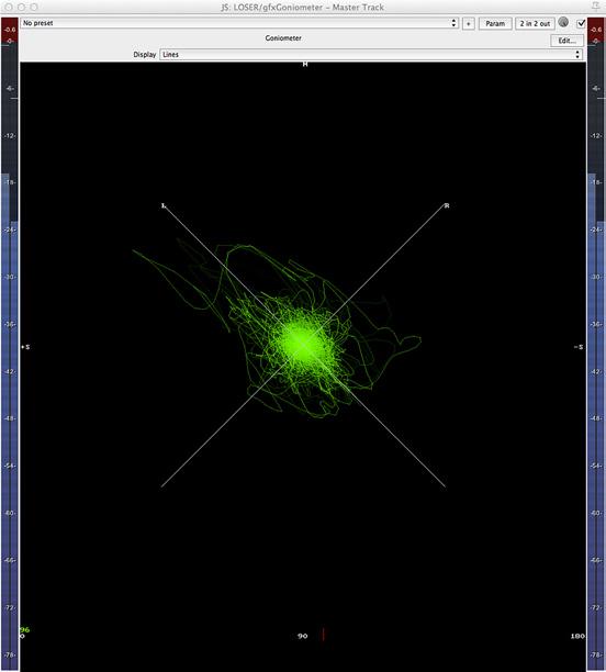
For my own recording and mastering work, I always have a goniometer in my line of sight (most also incorporate a phase correlation meter, by the way) and typically use it alongside a BBC twin-twin PPM. In my own studio I rely on an (obsolete) DK Technology MDS600M++ stereo vectorscope, but on location I use a TC Electronic Clarity M digital meter (or plug-ins if I’m working with a computer rather than a hardware recorder). On location, where auditioning is usually via headphones, the vectorscope meter is an essential tool for confirming stereo imaging information.

With an understanding of spaced and coincident arrays, we can exploit the characteristics of both — whether with established arrays or by designing our own.

Chapter 7

Hybrid Stereo Arrays

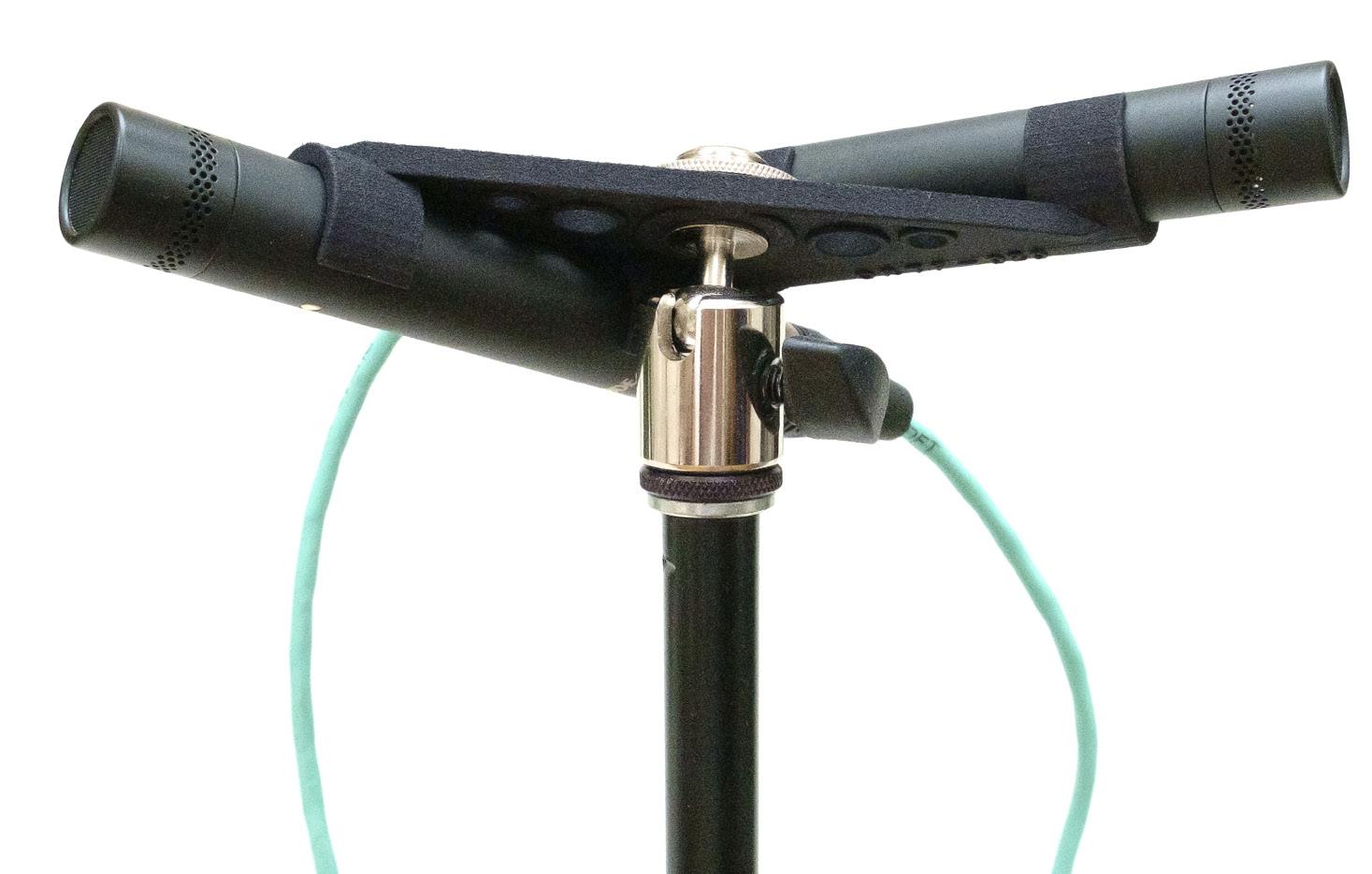
In previous chapters, we explored the concepts of coincident and spaced stereo mic arrays. I hope you’ll recall that while coincident arrays generally deliver stable and precise stereo imaging, they’re often described as lacking ‘spaciousness’; in contrast, spaced arrays excel in the ‘spaciousness’ department but their stereo imaging is typically vague and unstable.

There’s no technical reason, though, why these disparate approaches can’t be combined to create a ‘hybrid’ array — one which uses directional polar patterns set

with a mutual angle, but with the mics spaced apart. Indeed such stereo mic arrays are common and popular, and it’s probably fair to say that most recording engineers use them most of the time! As with all the other stereo arrays we’ve considered, there are no fixed rules; the recording engineer can employ any capsule spacing, polar pattern and mutual angle they think appropriate for any given situation, bearing in mind that these parameters interact to determine the Stereo Recording Angle (SRA) of the array, as well as the overall character of sound.

As with coincident mic array setups (crossed cardioids, Blumlein, Mid-Sides and so forth), there are many precisely defined and named hybrid mic arrays, most being devised by European broadcasters in the early 1960s and consequently named after those organisations.

Popular Hybrid Stereo Arrays

The best known and most popular is the ORTF mic technique, which was developed around 1964 by the Office de Radiodiffusion Télévision Française (the post-war French state broadcaster, which was broken

up into seven new broadcasting companies in 1974, including TF1, TF2, FR3, and Radio France). For this array, two cardioid capsules are spaced apart by 170mm, and face outwards with a 110-degree mutual angle to give an SRA of 96 degrees. At around the same time, in the Netherlands, the national broadcasting foundation (Nederlandse Omroep Stichting) came up with a variation on the same theme. This NOS configuration also uses cardioid capsules but they’re arranged with a 90-degree mutual angle and a 300mm capsule spacing, a combination that gives a slightly narrower SRA of 81 degrees. And in Germany, the Deutsches Institut für Normung standards institute came up with the DIN array. This also employs cardioids with a mutual angle of 90 degrees, but its slightly narrower capsule spacing

of 200mm gives a wider SRA of 102 degrees.

There are virtually limitless combinations of different capsule spacings, mutual angles and polar patterns, so not surprisingly there are other less well-known named formats, such as RAI (cardioids, 210mm spacing, 100-degree mutual angle) and EBS (cardioids, 250mm spacing, 90-degree angle). I’ve skipped over these simply because they’re so similar to the arrays I’ve already described, but I will highlight one more option, since I’ll be returning to it in the context of post-production signal processing in a later chapter. The Gerzon array employs cardioid capsules with a mutual angle of 120 degrees and a spacing of just 50mm, giving an SRA of 130 degrees. This array was named after and promoted in the 1980s by Michael Gerzon, a genius who’s probably best known as the

inventor of (first-order) Ambisonics and the SoundField microphone, and who credited the array to award-winning recording engineer and producer, Tony Faulkner. I wrote a detailed article about it in SOS November 2020, which you can read at www.soundonsound.com/ techniques/gerzon-array

To help you appreciate the practical differences between all these named arrays, Diagram 1 indicates a notional orchestra on stage (the yellow block) with each hybrid stereo array positioned such that its SRA encompasses the full width of the orchestra. Since these arrays all use cardioid capsules, I’ve also included coincident X-Y cardioids, with their nominal 196-degree SRA.

As can be seen, the NOS array’s relatively narrow 81-degree SRA means it must be placed furthest from the orchestra, with the X-Y

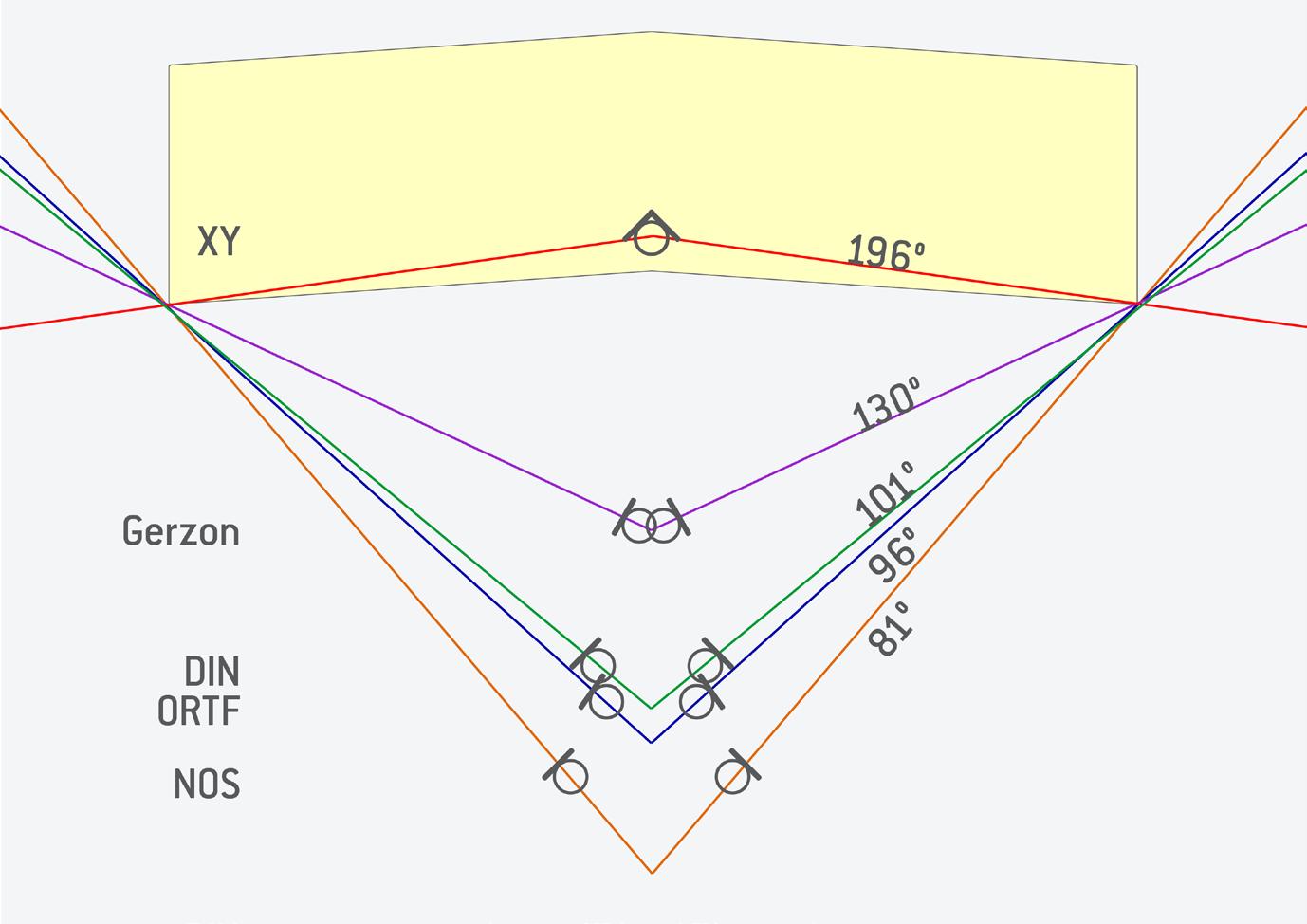
Diagram 1: The tighter an array’s SRA, the further back you must place it to have the source occupy the full stereo soundstage.

coincident cardioids being the closest (typically right above the conductor). Consequently, each of these arrays will deliver a similar stereo width when auditioned on speakers, but very different perspectives (direct/reverb balance) due to their different distances from the stage; the more distant placements capture more ambience and reverberation than the closer ones, but also have different degrees of ‘spaciousness’ due to their differing capsule spacing. Again, NOS offers the greatest spaciousness and X-Y the least.

Practical Mic Placement

But faced with so many options, how do you choose? As with coincident and spaced arrays, the basic principle of mic placement is to decide first on the desired perspective — how far away from the source(s) the mics should be for the optimum balance of direct to reverberant sound. When rigging and rehearsal time allows, you can assess that by listening to a single mic (of the type you intend to use for the stereo pair) facing directly forwards, with the monitoring switched to mono. Then adjust the placement (distance and height) to capture a sound with a nice overall balance of the ensemble on stage — but make it very slightly too dry, since it will sound more reverberant in stereo.

It can be very difficult to estimate the angle of the mics in a stereo array by eye, but a digital protractor makes precision quick and easy.

they align with the outer edges of the wanted soundstage while looking over the hinge. The display in the protractor gives me the exact angle required, and I can then refer to a stereo mic visualiser app to explore the various combinations of mutual angle and capsule spacing for my chosen mics’ polar pattern that match that SRA value.

“Changing from cardioid to subcardioid has a similar effect to reducing the mutual angle — because a sound source must be further away from the centre to generate the same inter-channel level difference.”

Having established the optimum position for the array, you can figure out the stereo recording angle needed to encompass the entire ensemble. I’m not great at estimating angles by eye, so I use a digital protractor made by GemRed (I’m sure other brands make similar devices). I stand where the mic array is to be located, and open the protractor’s arms until

Choosing a smaller capsule spacing means more of the stereo information is conveyed as inter-channel level differences, which means sharper imaging detail but less spaciousness. Selecting a wider capsule separation generates more inter-channel time-of-arrival information, so a greater sense of spaciousness but less image stability and precision. Changing the capsule spacing alters the SRA, of course, and that needs to be corrected by adjusting the mutual angle between the

capsules. In doing so, a smaller mutual angle gives a more uniform tonality across the stereo image (the stage sources are less off-axis). A larger mutual angle means far more of the wanted sound sources on stage will be being captured increasingly off-axis, and so may have a less consistent tonality. This depends on the consistency of the mic’s polar pattern with frequency, and I’d generally avoid large mutual angles when using large-diaphragm microphones for that reason, but when using good-quality small-diaphragm mics I find that it’s rarely a noticeable issue in practice.

A third variable, especially when using multi-pattern mics, is to change the capsule polar patterns. For example, changing from cardioid to subcardioid has a similar effect to reducing the mutual angle — because a sound source must be further away from the centre to generate the same inter-channel level difference. Swapping cardioid for hypercardioid is akin to increasing the mutual angle, and

narrowing the SRA. This extra option means we can add a third rule:

Rule 1: Reducing the Mutual Angle increases the Stereo Recording Angle.

Rule 2: Reducing the Capsule Spacing increases the Stereo Recording Angle.

Rule 3: Reducing the Pattern Directivity increases the Stereo Recording Angle.

Again, it’s important to remember that all of these parameters interact to some extent, so the ideal mic placement and array

Audio Examples

configuration is often arrived at iteratively. So my advice is to always allow yourself plenty of time to work through that process, auditioning the results at each step to make informed decisions and choices. Yes, the perspective and stereo imaging can be fudged somewhat in post-production, but it’s always far better to get it right at source, which is also the only way to arrive at the best possible sound quality.

With experience, it becomes easier to intuit an appropriate array close to the ideal from the outset. But building that experience takes

The media files associated with this book (https://sosm.ag/ stereo-recording-ebook) include an example of an ORTF hybrid mic array (Example 8, ‘ORTF’). This was captured using a pair of Rode TF5 microphones supported on a 3D-printed clip designed specifically for that purpose and mounted on the same stand that also accommodated the Mid-Sides array (Example 7, ‘Coincident Mid-Sides’). The latter makes a useful comparator for coincident versus hybrid arrays — but remember to adjust the Mid-Sides decoder to match the decoded stereo image width of the ORTF pair. Also mounted on the same stand was a pair of spaced omnidirectional mics (Example 11, ‘OCCO Omnis’), with a capsule spacing of 690mm for an SRA of 96 degrees — exactly the same as the ORTF array. Consequently, these spaced omnis allow a direct comparison between a pure spaced array and the hybrid ORTF setup.

Listening to the differences between these three alternative arrays, in terms of stereo imaging, spaciousness and perspective, can be very illuminating. Unfortunately, changes in tonality across the sound stage are almost impossible to perceive from these examples because of the relatively strong reverberation. But in drier acoustics, and with a wider sound source (for example, a full orchestra), those differences would be more apparent between the different arrays. Sadly, I didn’t have sufficient mics or recorder channels available to rig DIN, NOS and Gerzon hybrid arrays too, but hopefully this ORTF example will give a flavour of the benefits of hybrid arrays — and I would certainly encourage anyone interested in stereo recording to experiment with different configurations.

As mentioned, the ORTF, NOS and DIN arrays are very precisely specified. For example, if the capsules aren’t exactly 170mm apart and facing 55 degrees left and right, then it’s not an ORTF array. Rather, it’s a hybrid array of your own design. But if you find that 170mm spacing with a mutual angle of 120 degrees works nicely in a particular situation, there’s absolutely nothing wrong with using that combination. Just don’t call it an ORTF array!

a lot of time, experimentation and critical assessment in many different recording situations and environments! Recording is a craft and an art — it takes time to hone these skills.

Coming Up...

In the next chapter, I’ll discuss in more depth the practical considerations when choosing hybrid stereo arrays, examine the concept of ‘angular distortion’, and explore the potential of more sophisticated stereo arrays using more than two mics, including the famous Decca Tree.

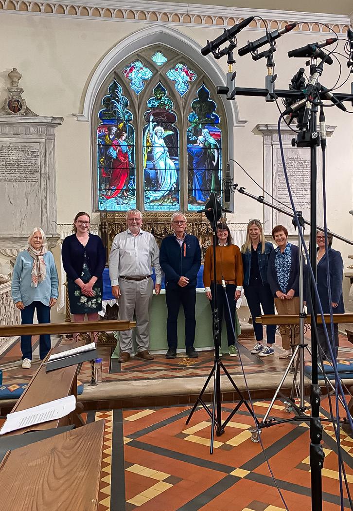
Thanks again to the Teme Valley South Churches Choir (TVSCC), who repeatedly performed ‘If Ye Love Me’ by Thomas Tallis to help us demonstrate the characteristics of various stereo mic arrays.

We dive deeper into the theory and practice of hybrid arrays, and consider the benefits of using more than one array.

Chapter 8

Advanced Hybrid & Combination Stereo Arrays

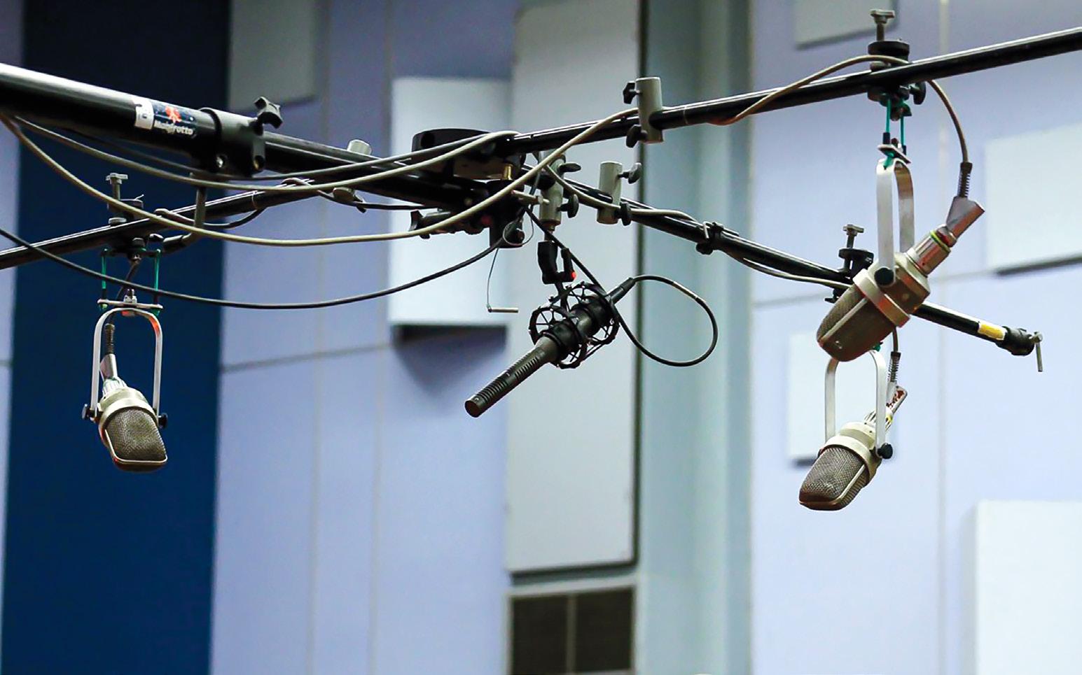
In earlier chapters, I introduced the concept of hybrid stereo mic arrays, and explored some of the initial practical processes that you can undertake to choose either an established named array — all of which are defined precisely — or to adapt the idea so you can tailor your own array to the recording task in hand. Now, it’s time to dive a little deeper into the subject, and we’ll start with some useful tools that can inform your choice.

Visualisation

In Chapter 6, I discussed some useful visualisation tools for optimising the SRA and capsule configurations, and the increased parameter interaction when tweaking hybrid arrays means good visualisation tools become even more helpful. However, there’s another way of looking at these things that I’ve found very educational and informative: The

Stereophonic Zoom. This was the title of an academic paper presented by Michael Williams to the AES Convention in London in 1984, and it has been enhanced by its author ever since, culminating in the excellent Multichannel Microphone Array Design book that I reviewed in SOS April 2023: www.soundonsound.com/reviews/ multichannel-microphone-array-de sign. That book covers a far wider range of mic configurations and applications than we’ve explored here, though, so perhaps an easier introduction to the concepts can be found in a PDF article available on Grace Design’s website: www.gracedesign.com/support/ StereoZoom10.pdf

Michael has, very generously, also published the associated graphs for a range of stereo arrays using different polar patterns on his website: www.williamsmmad.com/ MAD/2ch/2ch.htm. I’ve redrawn

one of his graphs for cardioid capsules configured in a stereo array (Diagram 1). The capsule spacing is shown along the bottom axis and the mutual angle along the vertical axis. The blue lines indicate the SRAs provided by different combinations of capsule spacing and mutual angle, while the orange blobs identify the parameters employed by the named hybrid arrays discussed previously.

As you can see, the X-Y coincident cardioid array, with zero capsule spacing and a mutual angle of 90 degrees, lies close to the blue 180-degree SRA curve. The DIN array, with its 20cm capsule spacing and 90-degree mutual angle, is offset to the right of the X-Y array, sitting close to the blue 100-degree SRA curve. Hopefully, examining this graph will help to make a little clearer how reducing the capsule spacing moves horizontally leftwards across the blue lines of

increasing SRA and, similarly, how reducing the mutual angle moves vertically downwards across the increasing SRA lines. The shaded areas at the top and bottom indicate the regions where the direct:reverb ratio varies across the stereo image. In the upper area there tends to be too much reverberation in the central zone of the stereo image, and the direct sound tends towards a ‘hole-in-the-middle’ effect. In the lower shaded area, the reverberation tends to increase and ‘pool’ towards the outer extremities of the stereo image. So, choosing parameters in these areas is not recommended.

Angular Distortion

The red lines, roughly perpendicular to the blue SRA curves, represent the ‘angular distortion’ created

by the array, indicated here as a percentage error from the true position. Angular distortion, in this context, is the variance between the physical angles between sources in front of the microphones, and their perceived relative angles when replayed over loudspeakers (see Diagram 2). It’s analogous to the optical distortion created by a wide-angle camera lens when it’s placed close to a subject.

As a general rule, most stereo mic arrays tend to expand the sound stage outwards — they push sources located away from the centre of the stereo image even further out towards the speakers, thus stretching the centre and ‘crushing’ the extremities. It’s usually a pretty subtle effect, but it’s certainly audible when comparing different array configurations in

good monitoring conditions. It can also become noticeable when close-miking a soloist who plays in an animated way, as any small physical movements can sound rather exaggerated when auditioned on the speakers.

The optimum conditions to minimise angular distortion vary with different polar patterns in the array, but for cardioid microphones the angular distortion is minimised by using moderate mutual angles (80-110 degrees) and capsule spacings (20-30 cm). In other words, hybrid arrays produce slightly less angular distortion than coincident arrays, and almost half as much angular distortion as spaced arrays. So it seems that capturing both time and intensity differences between channels is better than just time or intensity alone.

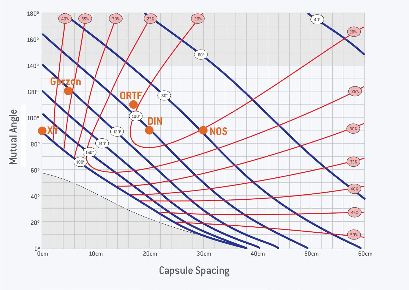
Diagram 1: The capsule spacing and mutual angle of various ‘name’ hybrid arrays. The shaded areas (top and bottom) indicate regions where the direct/reverb ratio varies across the stereo image.

Diagram

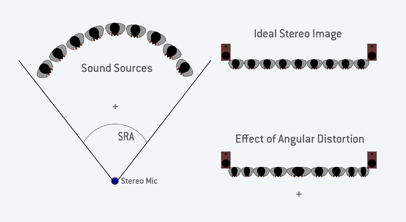
An illustration of angular distortion: sources further from the centre tend to be pushed outward towards the speakers.

As can be seen on the graph, the DIN array has the least angular distortion of all the hybrid arrays I’ve discussed so far, with NOS and ORTF both having a little more angular distortion. Not surprisingly, the coincident cardioids and Gerzon array have considerably more. In practice, this angular distortion is rarely even noticed, let alone problematic, but it’s still interesting to note how changing parameters affects this aspect of stereo-imaging accuracy. This angular distortion is also illustrated in the Sengpiel visualisation website mentioned in chapter 6 (https://sengpielaudio. com/HejiaE.htm). The five equally spaced coloured radial marks within the shaded SRA represent equidistant sound sources, and are replicated on a line between the two loudspeakers above, their spacing indicating the angular distortion created by the selected mic array configuration.

Combination Arrays

Spaciousness in a stereo recording is always a very attractive and desirable feature, but as I hope has

become clear, achieving a pleasing level of spaciousness will often compromise the stability and precision of the stereo imaging. Wouldn’t it be nice if there was a way to achieve the best of both worlds? Well, there is... but it requires additional microphones and might make the stereo purists go weak at the knees!

known for reasonably accurate stereo imaging — ORTF, for example — and supplement the spaciousness by adding more widely-spaced omnidirectional mics a little lower in the mix? The use of omnidirectional capsules also has the potential advantage of improving the low-frequency extension, making up for the known weakness in that

“The main risk, when adding extra microphones to an array, is the introduction of large phase differences between channels.”

The main risk, when adding extra microphones to an array, is the introduction of large phase differences between channels, which can then cause unwanted colorations (comb-filtering effects) when summed to mono. But if the level of the extra microphones is kept low (around 8dB below the main mics) those phase differences are unlikely to cause major problems.

So, why not rig a main pair using a near-spaced hybrid stereo array

area of cardioid microphones. Once again, there are many variations on this core theme, but a particularly popular configuration has become known as the OCCO array. The letters indicate the layout of two pairs each of omni and cardioid capsules. I’ve occasionally seen it called the ‘Optimal Cardioid Capsule Configuration’, although that seems rather lacking given the array requires omni capsules too!

I’ve never seen a precise definition of the OCCO array, but

most configurations employ the cardioids in a near-spaced format, usually ORTF (but occasionally DIN or NOS) at the centre, with the outer omni capsules usually pointing outwards at around 45 degrees and spaced as wide as the shared mounting bar allows (I typically use 660-690 mm; as in Diagram 3). APE spheres on the omnidirectional mics can be useful, if available, to enhance their stereo imaging definition (as in the Decca Tree arrangement — see box).

Typically, the ORTF (or similar) cardioid pair would be considered the main stereo array, and its position and settings would be optimised and balanced accordingly — but ‘erring’ towards a slightly dry balance, as the omni outriggers will make the mix more reverberant. The outer omnis are then blended in to the mix, usually 8-10 dB below

the ORTF pair, to add the required spaciousness, ambience and LF extension. An alternative but equally valid approach is to consider the spaced omnis as the main stereo array, optimised for perspective and imaging in the usual way. The central cardioids can then be blended in just to add a little focus and positional definition to the mix. Again, to avoid the risk of coloration in a summed mono mix, keep the second pair 8-10 dB lower in the mix than the main omnis.

Tony Faulkner, who I’ve mentioned previously in this series, has taken this idea further with an arrangement he calls a ‘Phased Array’ — a term borrowed from sophisticated techniques employed with multiple radio antennae, as well as in military radar and sonar systems. The idea is that by controlling the relative

phase relationships between transducers, it’s possible to ‘steer’ the directionality or focus of the entire array, although I’m not convinced that’s really what is going on in this application.

The particular configuration Tony suggests, which he has used for several orchestral recordings, places all four mics on the same bar, angled 45 degrees left and right (as shown at the bottom of Diagram 3), with the outer omnis spaced at 670mm and the inner cardioids at 410mm. With such a wide spacing, the SRA of the cardioids is only around 67 degrees, while the omnis have an SRA of around 100 degrees. Essentially the omnis act as the main stereo array, with the ability to blend the cardioids in to add focus and clarity to the centre of the orchestra as a kind of audio zoom control. Like the

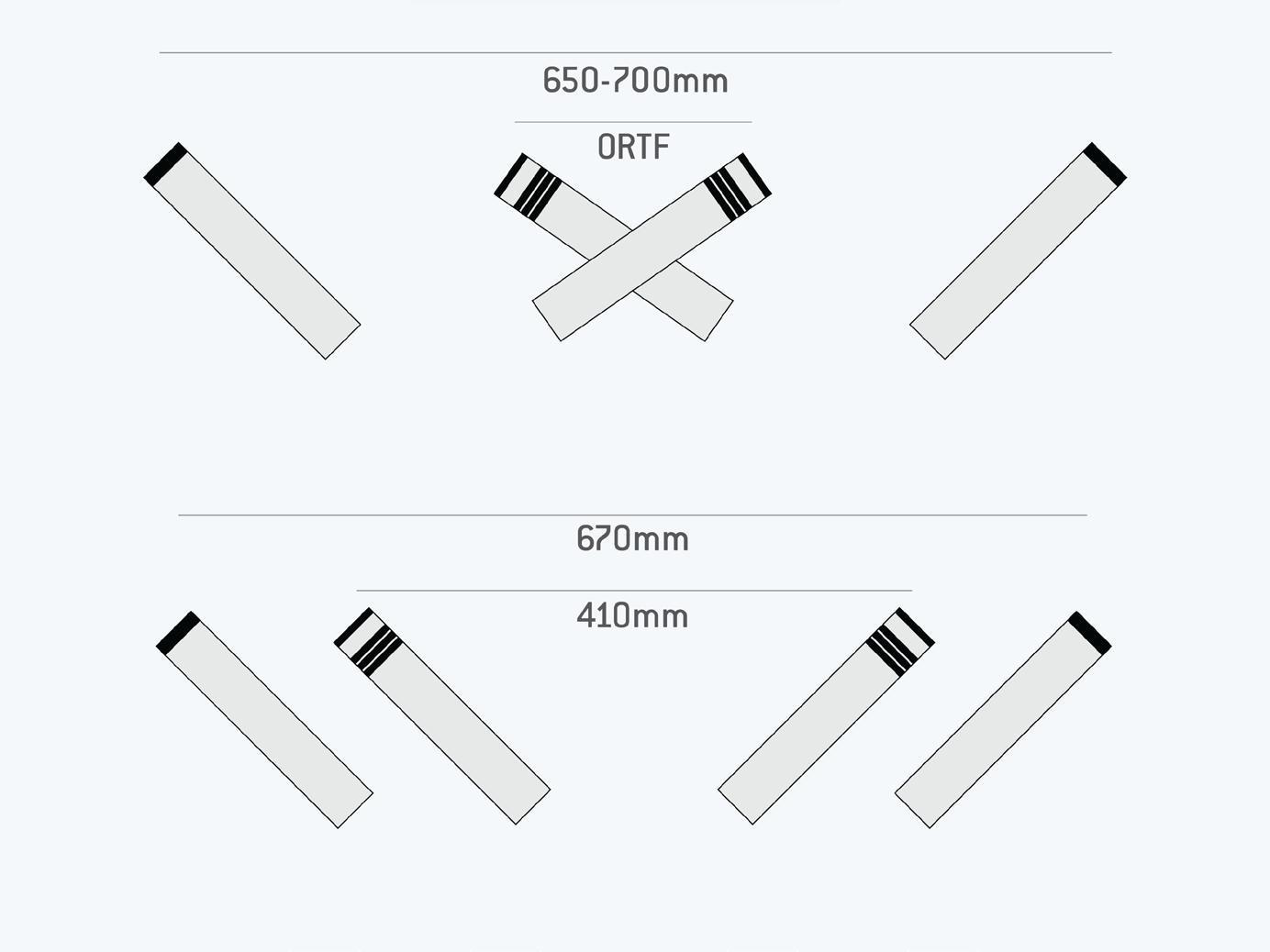
Diagram 3. Top: A typical OCCO array, with an ORTF stereo array complemented by omni outriggers. Bottom: A Faulkner ‘Phased Array’, with two pairs of mics mounted on the same bar and pointing 45 degrees left/right.

OCCO arrangement, this kind of multi-mic configuration is neat and quick to rig — it requires only one mic stand — but it affords a useful degree of flexibility in the output sound character, in terms of perspective, spaciousness and imaging definition.

Separated Arrays

Of course, there’s no rule that insists the omnis and cardioids must be mounted on the same bar; that’s just a convenience. Often the near-spaced array and the spaced omnis are deliberately separated, with one pair placed in front of the other (usually at the same height). This requires a more substantial and sophisticated mounting rig, but it’s a worthwhile investment because it opens up a whole new range of options.

There are multiple solutions to the mounting mechanics, but my preference is to use a pair of Manfrotto 154b mic bars. The first bar is mounted facing fore-aft on a tall Manfrotto light stand (1004BAC), allowing a stable 3.6 metres of height (when weighted adequately with sandbags!). The second bar is suspended from one end of the first, facing left-right with the omni mics near each end. At the other end of the fore-aft bar, I hang a short stereo bar for the near-spaced cardioids. The fore-aft bar is then adjusted to optimise the balance, keeping the centre of gravity of the whole assembly directly over the mic-stand centre. The Manfrotto mic bar is 650mm long, which is enough for most spaced-omni setups, but the supplied tubes can be easily

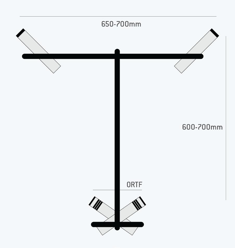
Diagram 4: Combining spaced omnis and near-spaced cardioids. The omnis offer a spacious, natural sound character and extended LF response, while the cardioids can be blended in for greater focus and image stability.

swapped out for longer 25mm aluminium or carbon-fibre tubes should greater mic spacing be required. The same idea can be used to build cost-effective and secure Decca Tree configurations.

An example of a combined array using separated spaced-omni and cardioid arrays is with the omnis spaced 650-700 mm apart and positioned around 600mm in front of the near-spaced pair, which could be in ORTF or DIN configuration (Diagram 4). The idea here is to match the perspectives captured by each mic array — the near-spaced cardioid pair inherently captures less reverb than the spaced omnis, so needs to be mounted at a greater distance from the source to have a similar amount of reverberation. Like the ‘Phased Array’, the omnis would typically be employed as the primary pair for their spacious and natural sound character with extended low-frequency reach, and the near-spaced cardioids blended in to supplement focus and imaging stability.

An equally valid yet reversed approach is to mount the near-spaced cardioids at the front, closer to the sound source, with the spaced omnis around 600mm (or more) behind. In this case the near-spaced cardioids provide the main stereo sound and the omnis are blended in to give more room ambience. This configuration has the advantage that the increased separation of the omnis behind the cardioids reduces coherence between the two stereo pairs, allowing a higher level of omnis in the mix before coloration occurs in a mono sum.

Coming Up...

In the next chapter, we’ll look at some of the post-production processing options that can be used to further enhance or correct the stereo imaging obtained by the myriad coincident, spaced, hybrid and separated stereo microphone arrays I’ve described throughout this book.

The Decca Tree

When discussing the concepts and applications of spaced omnidirectional microphones in this and the previous article in this series, I have deliberately avoided all mention of the Decca Tree array — even though it employs spaced omnidirectional microphones. The reason is that the true Decca Tree arrangement is actually a lot more complex than many realise, and requires specialist omnidirectional microphones fitted with Acoustic Pressure Equalisation spheres to work properly. The technique really deserves an entire chapter all of its own, but if you are interested in learning more about it I can highly recommend the book ClassicalRecording: A Practical Guide In The Decca Tradition by Haigh, Dunkerly and Rogers, which I reviewed in Sound On Sound in March 2021: www.soundonsound.com/ reviews/classical-recording-pract ical-guide-decca-tradition

Most think of the Decca Tree as a simple three-mic array but, when employed for large orchestral recordings it’s really a complicated six-mic array. The familiar three-mic tree is suspended above the conductor, but it also requires two additional omni outriggers positioned left and right (between the second and third desks of violins and cellos), plus a sixth mic positioned above the double basses. That combination, along with the specific microphones used, delivers the famous Decca Tree’s sound character. The dimensions for the central ‘tree’ vary depending on the situation, but for a typical orchestral setup the left and right mics are generally spaced around 1300-1400 mm apart (although I have seen wider spacing in some commercial recordings), with the centre mic placed forward by half of the left-right mic spacing.

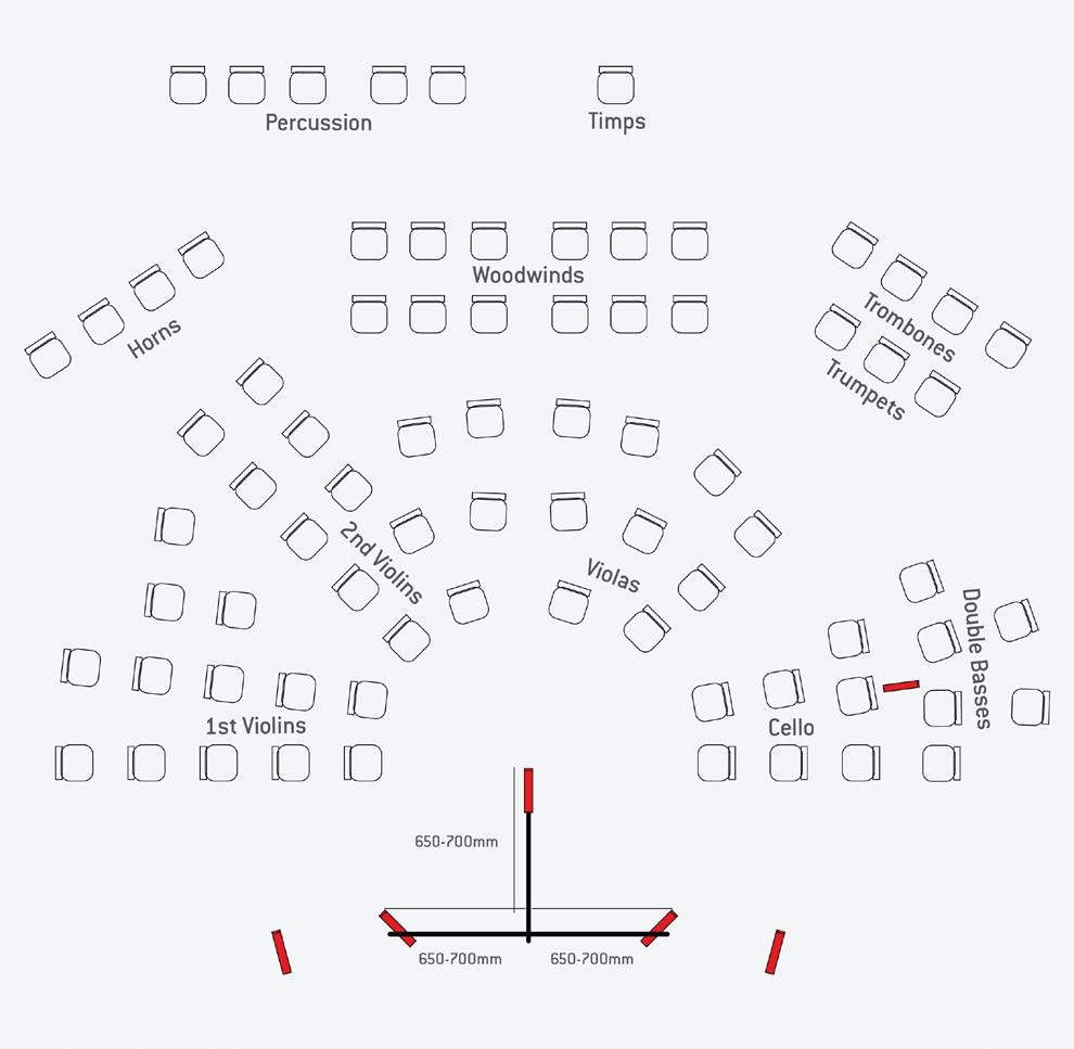
A full Decca Tree setup, with a central three-mic tree joined by a pair of omni outriggers on either side, and a sixth mic placed above the double basses.

For a small ensemble, like a string quartet, a simpler three-mic tree can be employed, with the left-right mic spacing reduced to around 600mm, and the centre mic around 150-200 mm forward. However, I’ve often found this mini-tree approach less pleasing than other hybrid arrays for recording small ensembles. Mounting the centre mic forward of the left and right pair is a very clever design feature of the Decca Tree. Spaced omni microphones can easily form a hole in the centre of the stereo image if spaced too widely, and the centre mic neatly fills that potential hole in the sound coverage. But more than that, by being

slightly forward of the other two it captures sound fractionally earlier by a millisecond or two, greatly enhancing the stability of the stereo image because the reproduction over loudspeakers builds the stereo image from the centre outwards.

Traditionally, the omni mics employed in a Decca Tree are Neumann M50s, which house the omni capsule within a 40mm sphere, and this is critical to the performance of the array. The sphere not only boosts the microphone’s high-frequency response but also narrows the directivity at high frequencies. So, these omni’s are directional, and this is the reason why the omni mics are angled left/right at roughly

45 degrees from the centre. In the six-mic array, the outriggers are also angled slightly outwards by about 15 degrees, and this capsule angling is critically important in generating a coherent stereo image. Most small-diaphragm omni microphones can be fitted with APEs — either as manufacturer accessories or as 3D-printed options — and I strongly recommend this approach if you don’t have access to M50s or equivalents. At a push, subcardioids or even cardioids can be used instead, maintaining the capsule spacing and HF directionality, but at the cost of the LF extension and phase linearity associated with omnis.

Chapter 9 Replicating Human Hearing

For this final chapter on stereo miking, we explore the world of binaural recording, disc-shaped baffles and dummy heads.

The preceding chapters of this book took us on a journey from the fundamental concepts of stereo sound recording and reproduction to the theory and practical aspects of a wide range of stereo microphone techniques. We’ve explored Blumlein’s coincident arrays, including Mid Sides, which focus on capturing and reproducing only amplitude differences between channels; and the wide spaced omni mic arrays that capture mainly time of arrival differences between channels. We went on to consider a number of popular near spaced arrays that were designed to combine both amplitude and timing differences between channels — the best of both worlds — before also contemplating some of the more complex stereo mic arrays that combine both spaced omnis and near spaced arrays, including a brief look at the famous Decca Tree. By this point, then, you’d be forgiven for thinking that there couldn’t possibly be any more stereo mic arrays to examine! But there are — and if you’ve been working through the audio example files associated with this book, you’ll already be aware of one example: the Schneider Disc. This, with variations upon it, is the last stereo mic array that I want to discuss in this series, as it represents

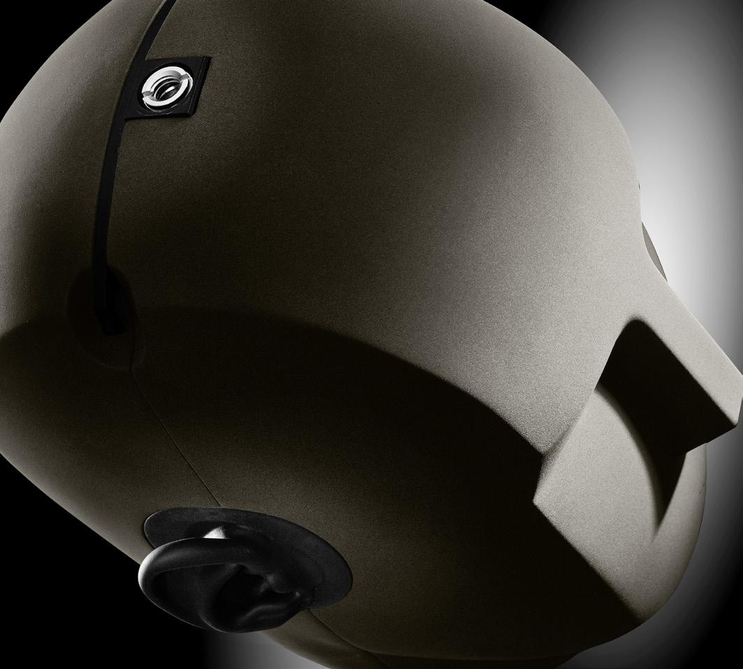
a final class of stereo microphone techniques that aim to replicate the human hearing physiology — to a greater or lesser extent.

Dummy Head

If the idea of stereo recording is to replicate the human experience of listening to performers on a stage, arguably the most obvious approach is to imitate the human listening apparatus. Basically, that means using a head shaped construction with microphones in place of the ears. This concept, popularly known as the ‘dummy head’, has been explored in depth for decades, and there are several commercial examples, including Neumann’s original KU80 and current KU100, and Sennheiser’s now discontinued MZK2002, amongst various others.

These dummy head systems produce a stereo signal in a format generally referred to as ‘binaural’,

which is intended exclusively for headphone listening. However, the success of these dummy head recordings, in terms of imaging stability and source location realism, depends very heavily on how closely the listener’s anatomy matches that of the dummy head, particularly in terms of head size and ear spacing (early dummy heads don’t attempt to replicate the folds and curves of the pinnae which, as we know, play an important role in vertical and front/back source location).

The physiological parameters of the listener’s head/ears determine what is now known as the ‘Head‑related Transfer Function’ or HRTF, which is unique to each individual listener, and it is these parameters that define how we individually perceive sound locations within a binaural signal.

As it happens, I own a Sennheiser MZK2002 dummy head. The recordings I’ve made with it certainly sound spacious and are interesting,

but I don’t find them consistent, stable or precise. That’s probably in large part because the dummy head is physically smaller than my own. If I attach the same Sennheiser microphones to my own ears for recording, then playing back the audio files gives me remarkably precise and stable imaging information. But it’s important to note two things... First, if you move your head at all, you change the perspective of the mics. And second, this approach benefits me alone — others who’ve listened to recordings I’ve captured that way usually find the imaging to be imprecise and unstable again. This highlights the critical importance of personal HRTFs for accurate spatial imaging in binaural listening.

Today, of course, there’s a huge academic and commercial interest in binaural stereo, not least because of the vast numbers of people who now listen over headphones habitually. And while personalised binaural recordings might not transfer well from one listener to another, binaural reproduction is an ideal format for low-cost immersive-audio playback. Indeed, with the benefit of sophisticated digital signal processing, and the ability to create and implement personal HRTFs for playback over headphones, binaural stereo is making significant headway in popularity, and many manufacturers are now incorporating this technology in smartphones, tablets, laptops and more.

One down side of binaural stereo and dummy-head recordings, though, is that the format is specifically intended for use with headphones, and the stereo imaging is usually very poor when auditioned over loudspeakers. That wouldn’t be a problem if the entire audience were known to use headphones, but in most cases a significant proportion of the audience for commercial music is likely to be listening over loudspeakers. So is there an alternative technique that could offer better compatibility

between headphone and loudspeaker listening?

Optimal Stereo Signal (OSS)

Take away the physical differences between individuals’ heads and ears, and the main significance of the replica head in dummy head recordings is that it acts as an acoustic baffle, reducing the strength of high frequencies from a source on one side reaching the ear on the opposite side, as well as introducing a time delay to the further ear. So why not just reduce the ‘dummy head’ to its simplest form: a flat baffle, with microphones placed on either side?

Needless to say, it’s been done... and as you might already have guessed, the first person to do it was Alan Blumlein, back in the early 1930s. One of his earliest experiments involved a pair of pressure (omnidirectional) mic capsules separated by an acoustic baffle. He described the setup in his famous patent, along with sophisticated signal processing to

make it work better for loudspeaker listening, which is something I’ll come back to shortly. It wasn’t a line of enquiry Blumlein pursued at the time, though, as he chose instead to focus his work on coincident velocity (directional) microphones, which, to his mind, gave better results with loudspeaker auditioning. But good ideas have a habit of resurfacing sooner or later, and it was the work of Jürg Jecklin in the early 1980s, at the University of Music and the Performing Arts in Vienna, that resurrected the interest and popularity of Blumlein’s idea. He called the technique the Optimal Stereo Signal or OSS — but it became far better known for its physical appearance, and is usually referred to simply as...

The Jecklin Disc

Jecklin’s earliest design employed a flat, 30cm diameter disc, covered in a thin layer of foam (or fleece) to reduce the baffle’s acoustic reflectivity. A pair of omnidirectional microphones were then mounted on

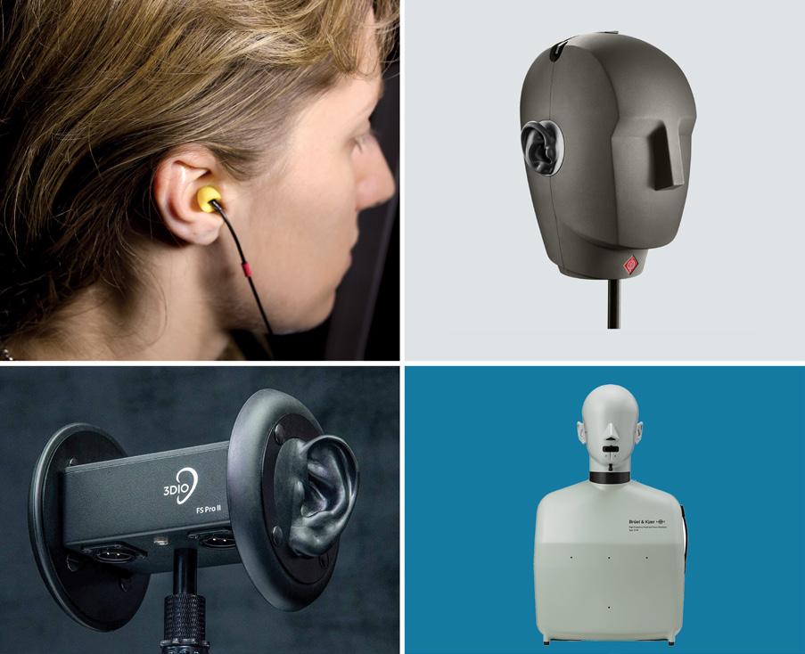
A range of mics intended to replicate the human listening experience. Clockwise from top right: the Neumann KU100 dummy head; Bruel & Kjaer’s HATS system; the 3DIO FS Pro II; and some ear-worn mics. The last of these could potentially be the most convincing — but only for the person who wore the mics!

either side of the disc, their capsules being aligned with the centre of the disc, spaced 16.5cm apart (so roughly 8cm above the disc’s surface) and pointed outwards by 20 degrees.

In essence, the disc baffle broadly replicates the primary acoustic effects of the human head, with the baffle diameter and mic spacing combining to introduce similar frequency response, time and amplitude differences between the two microphone signals as are experienced at the ears of a listener. Those differences increase as a sound source moves further off axis from the front of the disc, much like it does with human hearing.

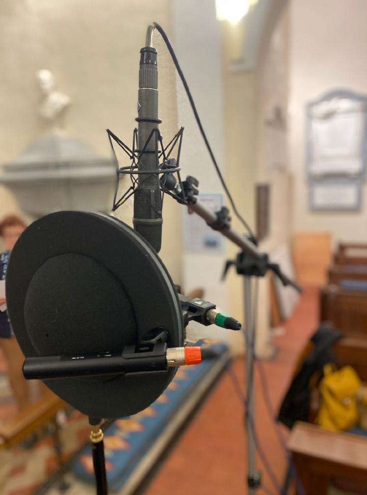
Most commercially made OSS discs follow Jecklin’s original specifications for the baffle size and mic spacing, but in the mid-1980s Jecklin himself revisited the design, and concluded that it performed better with a larger baffle diameter and greater mic spacing. Consequently, he issued revised specifications, with a disc diameter of 35cm, and mic spacing increased to 36cm (so roughly 17cm above the disc surface).

Commercial Jecklin Discs are not inexpensive, but anyone handy at basic DIY can construct their own experimental Jecklin Disc relatively easily, using something like a piece

In the foreground is the Schneider Disc array (a variation on Jecklin’s original OSS technique) used for example 10 in the audio recordings that accompany this book.

of plywood or Perspex cut into a disc. While the size/diameter is fairly important, you don’t even need to be able to cut a perfect circle (the human head is broadly ellipsoid rather than spherical, after all). A handle or mic stand mounting thread can be attached to the disc, along with a pair of threaded studs or tubes mounted near the back to support standard mic clips. Their positioning needs to accommodate the length of the intended omni mics such that their capsules end up near the centre of the disc when angled outwards by 20 degrees. The plywood or Perspex disc casts

“One down side of binaural stereo and dummy-head recordings is that the format is specifically intended for use with headphones, and the stereo imaging is usually very poor when heard over loudspeakers.”

an acoustic shadow, but as it also reflects sound, it can then be covered with some acoustic foam and/or fleece on each side. Then your Jecklin Disc is ready for use!

Schneider Disc

As always when it comes to stereo mic techniques, there are several variations on this theme, and audio example 10 in the demonstration files associated with this series (https://sosm.ag/stereomiking-demo-files) was captured using what’s known as a Schneider Disc, a version of the OSS technique that’s very similar to the standard Jecklin Disc. The baffle diameter is the same as the original Jecklin specs, and the mic spacing is the same too. However, in addition to the flat layer of foam on each side of the baffle, a hemisphere of foam is added at the centre of the baffle on each side. The idea of this extra foam is to better replicate the acoustic absorption effects of the human head. To be honest, the audible difference between a Schneider Disc and a Jecklin Disc is very subtle. My own view is that the Schneider version performs slightly better, particularly for headphone listening, but there’s really not a lot in it! (If going down the DIY route suggested above, you could always conduct your own experiments with different absorptive material...)

Jecklin recommends that the ideal placement of the (Jecklin or Schneider) Disc is at the room’s ‘critical distance’ (Dc) away from the source — where its direct sound and diffuse (reflected) sound are equal in strength. Personally, I prefer a slightly closer placement in most cases, but that’s an aesthetic choice, and one that depends on the nature

of the music and source, and the sound perspective required. For the Schneider Disc demonstration in the associated audio files, I mounted a pair of Sennheiser MKH 20 omnidirectional mics on the disc, spaced roughly 17cm apart with the disc positioned just above head height, and (because it was a particularly reverberant church, making the Dc distance relatively short) around 2.5 metres in front of the choir.

I have enjoyed good results using the Schneider Disc on small ensembles, particularly if the main audience is likely to be headphone users. However, the OSS system also works nicely as a main stereo array for larger ensembles, with excellent bass extension and a nice spaciousness that still works reasonably well on loudspeakers. The recording setup always attracts attention at public concerts, too (not because it’s particularly obtrusive; it’s more that people don’t see it used very often so are curious).

Stereo Shuffling

One of the reasons Blumlein didn’t pursue his baffled-omni-mics idea was because it didn’t generate purely level differences between the two channels at all frequencies — you’ll recall from earlier chapters that accurate stereo imaging from loudspeakers primarily relies on reproducing only amplitude differences between the two channels.

For off-axis sound sources, the baffle placed between the omni mics naturally introduces amplitude differences between channels at mid and high frequencies (where the wavelength approaches the baffle diameter). However, at lower frequencies the soundwaves simply diffract around the baffle, resulting in negligible amplitude differences between the two omnidirectional mics. Thus, low-frequency sources appear to come from the centre of the stereo image, with negligible stereo width.

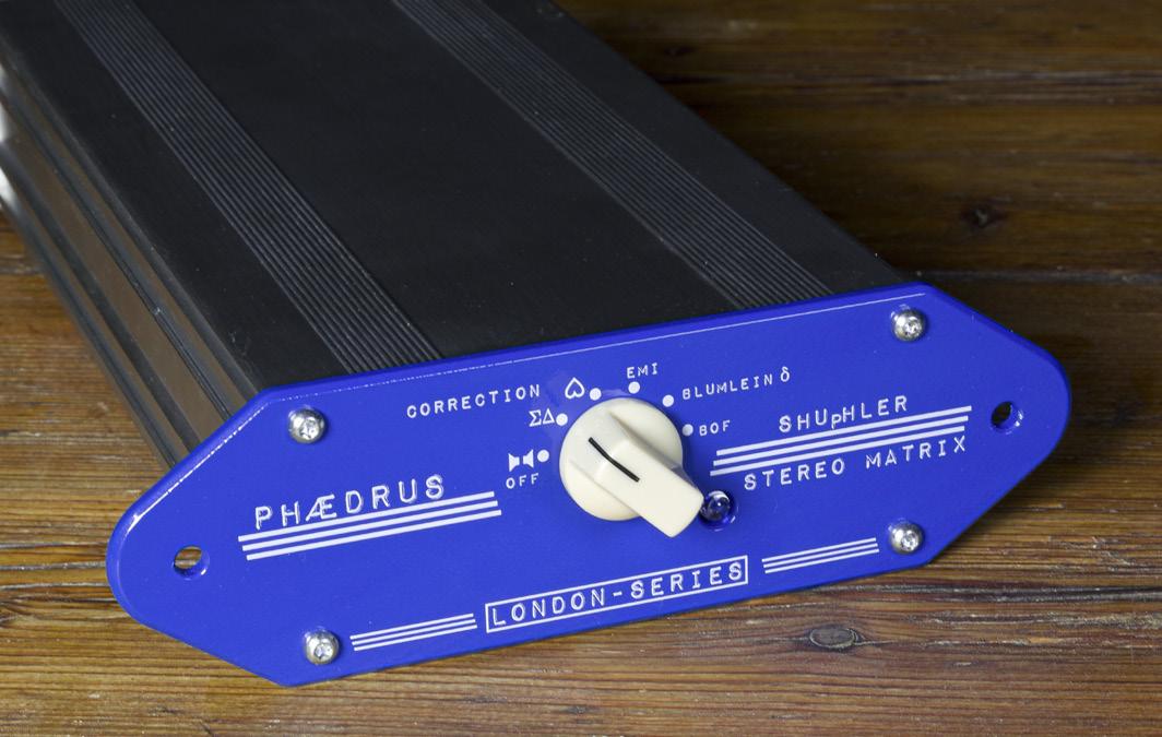
Nevertheless, the mics capture some low-frequency directional information because their physical spacing generates small phase differences at low frequencies, due to the different time-of-arrival of sound wavefronts at each mic. In an attempt to improve low-frequency stereo imaging over stereo loudspeakers, Blumlein developed a method of converting those low-frequency phase differences between channels into representative amplitude differences, and named this process Stereo Shuffling. As I mentioned earlier in this book, this Shuffling term has been used in a few different contexts and applications over the years, and that’s naturally led to confusion in some quarters! But the underpinning concept of all Shuffling processes is that they provide a frequency-dependent stereo-width correction.

Blumlein’s original Stereo Shuffling system worked in three distinct stages. First, the left-right stereo signal from the microphones was converted into the Mid-Sides format. Second, the amplitude of low frequencies in the Sides channel only was boosted, typically by around 8dB below 600Hz, using a first-order (6dB/oct) low shelf. Finally, the processed result was

Phaedrus Audio’s SHUpHLER, based on Blumlein’s Stereo Shuffler idea, can restore to recordings the sense of low-frequency stereo definition that’s often lost on loudspeakers.

converted back into left-right stereo. This frequency-conscious Mid-Sides processing cleverly converts the small phase differences between channels into significant amplitude differences, thus allowing much better stereo imaging when heard over loudspeakers. The size of the baffle determines the frequency above which the mics capture amplitude differences between channels and, for a head-sized baffle, that’s above about 600Hz; below that it’s just phase differences — hence using that frequency as the corner of the shelf EQ.

Other Shuffling Applications

As we’ve seen in previous chapters, various other stereo mic arrays also have inherent frequency-dependent stereo image width issues, and the same Shuffling concepts can often be used to help correct or improve the stereo imaging for loudspeaker listeners when using those recording systems. I mentioned in chapter 3, for example, how Stereo Shuffling can be employed to correct the tendency of directional mics to lose their directionality at low frequencies in coincident arrays, and how it can also compensate for the high-frequency beaming associated with figure-8 ribbon mics in a Blumlein array. The same technology also works

K S M S T U DIO MICROPHONE S

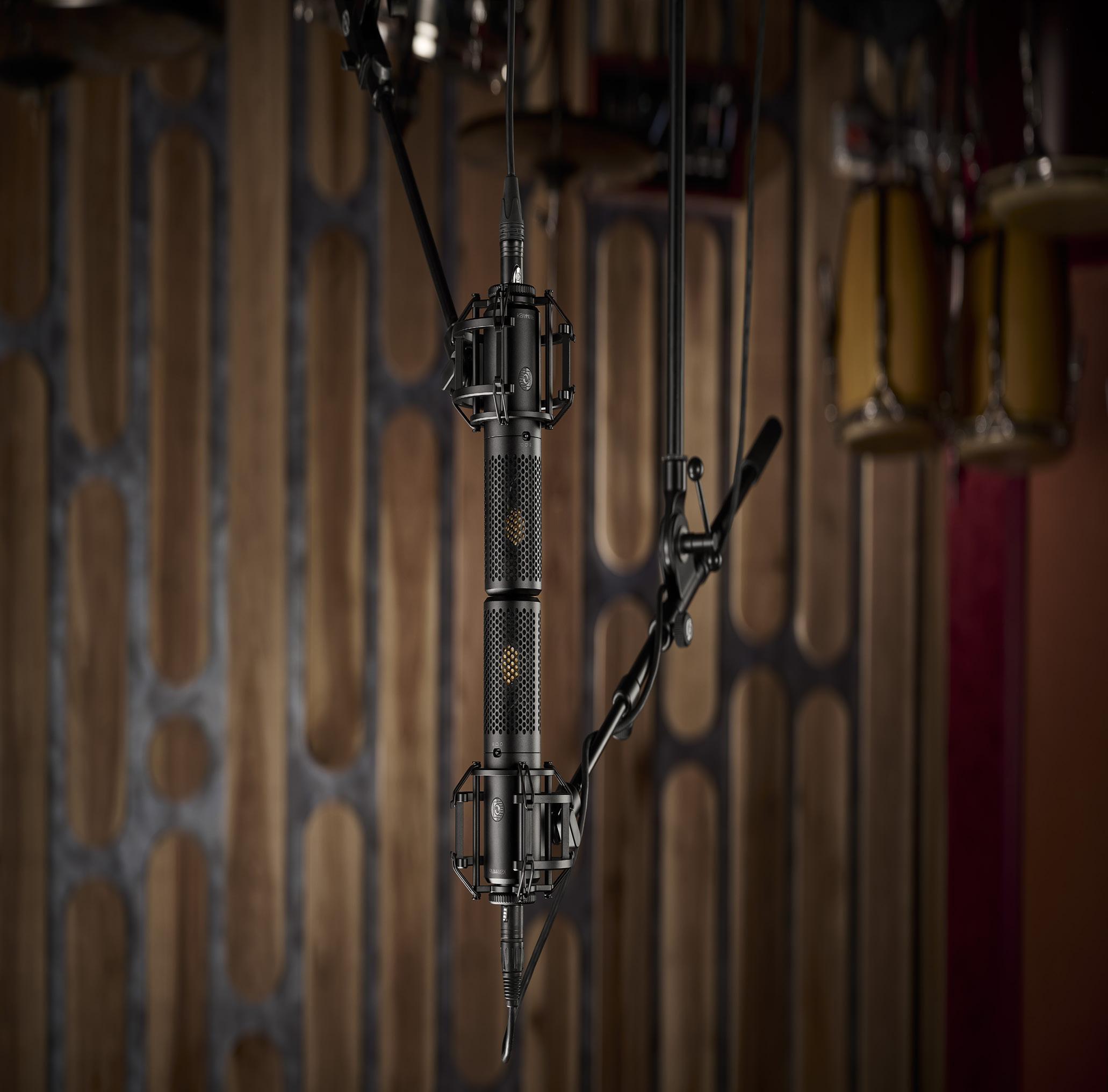
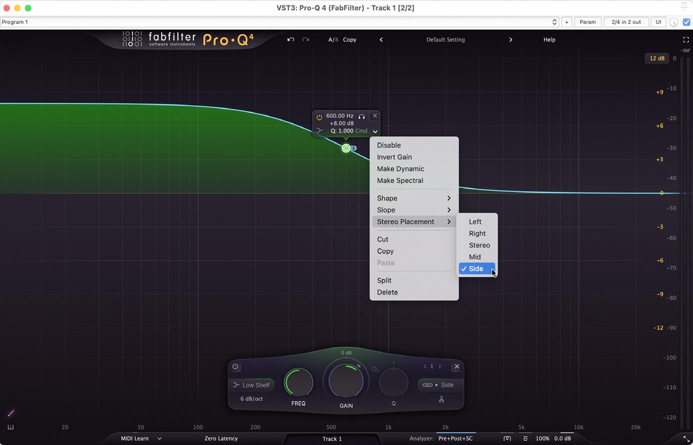
You can recreate the Stereo Shuffler effect in your DAW, either by putting an EQ between Mid-Sides encoder and decoder, or by using an EQ plug-in that allows you to process the Sides signal separately.

particularly well with the Gerzon array, for example, which I described in detail in SOS November 2020 (https://sosm.ag/the-gerzon-array).

One ‘problem’ with the Shuffling process is that, unless using a linear-phase EQ, phase-shifts occur whenever an EQ circuit is used (so it’s inherently an issue when implemented in analogue circuitry). If only the Sides signal is processed, that path incurs phase-shifts that aren’t replicated in the Mid path, and when the two signals are recombined to produce left-right stereo those phase-shifts can affect the overall tone in unhelpful ways.

In the case of the Gerzon array, the Sides channel bass boost EQ used in the Shuffling correction introduces around 25 degrees of this ‘phase lag’ at 600Hz. That’s a part of the spectrum where human hearing is relatively sensitive to phase shifts. Fortunately, the 5cm capsule spacing employed in that array introduces

a similar amount of ‘phase lead’ in the (converted) Sides channel, effectively counteracting the effect and minimising any phasiness in the processed and decoded output.

If applying Shuffling in a DAW, one can of course choose to use linear-phase filters in the Sides path. These don’t introduce frequency-dependent phase-shifts, but they will inherently introduce latency. Modern DAWs can correct that automatically on playback, but if they don’t (for example if you choose to bypass automatic latency compensation while recording), there may well be obvious comb-filtering artefacts in the decoded left-right output. Sometimes, applying a complementary cut in the Mid channel to balance a reduced boost in the Sides channel can give better results than processing only the Sides channel.

It’s fun and also educational to construct Stereo Shufflers in the DAW

from a combination of M-S matrix and EQ plug-ins — and there are plenty of EQs that can act separately on the Sides signal now of course. I’d encourage you to experiment with the amounts of boost (or cut) and the corner EQ frequencies — there are no rules, only good or bad results!

If you’re looking for an easier life, Pspatial Audio’s Mac-only Stereo Lab 4+ software contains myriad stereo processing tools intended for 78rpm records, modern RIAA vinyl, CD de-emphasis, tape and cassette processing, headphone enhancement, surround upmixing, and much more. It also includes a number of different Shuffler configurations, including modes optimised for coincident figure-8 and cardioid mics, as well as several variations on Stereosonic shuffling to improve loudspeaker monitoring. I highly recommend it.

For real-time Shuffling, there’s Phaedrus Audio’s SHUpHLER,

the original version of which I reviewed in SOS July 2017 (www. soundonsound.com/reviews/ phaedrus-audio-shuphler). The latest version of this compact unit can be switched between several different Shuffler configurations, mostly the same as found in Stereo Lab, albeit without the linear-phase models. It processes the audio entirely in the analogue domain for real-time applications. Blumlein’s Shuffler for baffled spaced omnis is called Blumlein δ (delta) and it can be used on most near-spaced stereo mic arrays with good results. An alternative Shuffler, marked with an inverted heart symbol, has been optimised for coincident cardioids, but can also be useful with near-spaced cardioid arrays. The entertainingly named Bride Of Francinstein Shuffler is a modern take on EMI’s Stereosonic Shuffler, to help correct for the inherent stereo imaging compromises of loudspeaker listening. A fifth mode provides a straightforward Mid-Sides matrix.

Stereo Width Adjustment

When I discussed the Mid-Sides stereo mic array in chapter 4, I explained how changing the relative balance of the Mid and Sides channels altered the effective Stereo Recording Angle (SRA). In exactly the same way, if a left-right stereo signal is converted to Mid-Sides, adjusting the Mid:Sides ratio alters the width of a decoded stereo signal when auditioned over loudspeakers. This is a very useful facility that’s built into the stereo channels of some sound consoles, and most DAWs include a stereo width plug-in (if not, try Voxengo’s freeware MSED) that can be used for the same effect. Altering the stereo width in this way with material created using pan-pot stereo or a coincident stereo mic array source is inherently problem-free; there are no adverse stereo imaging side-effects to worry about unless the Sides signal is increased too much, resulting in a very out-of-phase sound

with a hole in the middle of the image. A phase meter or stereo vectorscope is the ideal visual aid to ensure the stereo width stays within sensible limits! Introducing an equaliser into the Sides channel, to increase the stereo width below about 600Hz, generally has a very beneficial effect on the sense of spaciousness in a recording — another use for Shuffling!

However, increasing the stereo width in this way with near-spaced stereo mic array sources can introduce significant problems, and should be used with great care. The fundamental problem is that, as the microphone capsule spacing inherently introduces significant phase-shifts between the two channels, at a certain frequency (and its higher harmonics) the phase-shift will approach 180 degrees. Because the Mid-Sides conversion involves sum-and-difference processing, those frequencies will create deep notches or peaks in opposite channels in the decoded stereo signal. So, while increasing the proportion of the Sides signal relative to the Mid will increase the stereo width at low frequencies, it will also alternately narrow and widen the signal at higher frequencies, potentially resulting in a substantially degraded and confused stereo image!

The only way to avoid this problem with near-spaced arrays is to restrict any stereo widening effects to the lower frequencies, where the phase-shift gets nowhere near 180 degrees. The maximum Sides channel turnover frequency that can be safely used can be calculated from: Hz = 5400/d

In this equation, d is the capsule spacing in centimetres. So, for example, the highest acceptable frequency for stereo-width enhancement of an ORTF array is 317Hz (5400 / 17). For an NOS array it would be 180Hz... and so on. The wider the capsule spacing, the lower the safe processing frequency. That said, with very

widely-spaced mics (say, over 1.5 metres) the signals in the two channels are so highly decorrelated that the phase-cancellation of higher frequencies ceases to be a problem.

To sum up, then, using Mid-Sides processing to change the width of a stereo signal works well with coincident mic recordings and with pan-pot stereo material, where there are no significant phase differences between channels. But, where there are deliberately introduced phase differences due to microphone capsule spacing, stereo widening should be applied with great care, paying attention to the stereo imaging of the mid and higher frequencies, which may become excessively wide or narrow. If this occurs, restrict the width enhancement to the lower frequencies only, according to that formula above.

In Conclusion

And with that, here endeth our lessons on practical stereo microphone techniques. Along the way, I’ve tried to point you to several other resources that I’ve found very helpful, and there are plenty more available on the web and in the bookshops — and some will include details on some more esoteric arrays, such as the Double Mid-Sides array and the Blumlein-Pfanzagl-Triple array, which might well be worth your while exploring if you want to journey further down this road.

Hopefully, though, the preceding chapters have helped to demystify many aspects of stereo miking. I also hope this book will encourage you to experiment more confidently with a greater range of techniques. Remember that there really are no rules, just options: the end results are all that matter. Armed with an understanding of the benefits, possible pitfalls and potential for modification of different arrays, you should be able to capture exactly the results you desire. Happy recording!

These demonstration recordings illustrate the effect of different array choices and distances on the sound character and stereo image.

HUGH ROBJOHNS

To illustrate the differences, strengths and weaknesses of different stereo mic arrangements, I made a series of demonstration recordings captured over about an hour on a warm summer’s evening.

The choir is the Teme Valley South Churches Choir (TVSCC), founded and conducted by Chloe May Evans. The location is a hilltop church in Worcestershire, UK, that’s pretty reverberant. Although it sounds very pleasant, that reverberation does make it a little harder to hear the stereo imaging differences. Nevertheless, I am immensely gratefully for the enormous generosity and patience of this excellent choir as they performed the same piece, ‘If Ye Love Me’ by Thomas Tallis, repeatedly in front of a number of different mic arrays, some being reconfigured and/ or physically moved between takes.

The different tracks and their noteworthy characteristics are described in detail in the preceding chapters, but the brief file descriptions here will also give pertinent clues. The microphones used in examples 1-12 are Neumann SM 69 FETs, Rode TF5s, and Sennheiser MKH 20s, 30, and 40s. The MKH 20s were switched to their diffuse-field mode, with HF boost. The wide omnis and SM 69 were recorded onto a Nagra VI, while the rest were captured on a Zoom F8n Pro. All of the files are 24-bit/48kHz, with no processing other than a little gain adjustment for approximate level matching.

To hear the audio examples listed please find them hosted on the Sound On Sound website, where you

Audio Demonstration Files

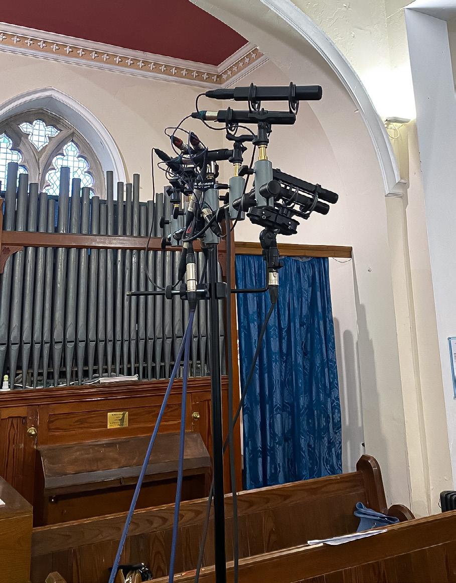
can also download the full-resolution WAV files in order to make direct comparisons in your DAW software: https://sosm.ag/stereo-mikingdemo-files

Coincident Stereo Mic At Distance

1. Neumann SM 69 Figure-8s

2. Neumann SM 69 Hypercardioids

3. Neumann SM 69 Cardioids

Coincident Stereo Mic At Different Distances

4. Figure-8 distant SM 69

5. Hypercardioids mid-way SM 69

6. Cardioids closest SM 69

Coincident Mid-Sides

7. Sennheiser MKH 40/30

(not decoded, Mid on Channel 1)

Near Spaced Arrays

8. ORTF (Rode TF5s)

9. Faulkner Cardioids* (Sennheiser MKH 40s)

10. Schneider Disc (Sennheiser MKH 20s)

*The Faulkner omnis are intended to be used in combination with the OCCO wide-spaced omnis as a phase array.

Wide Spaced Arrays

11. OCCO Omnis (Sennheiser MKH 20s)

12. Wide Omnis (Sennheiser MKH 20s)

BBC Pattern Demo

13. BBC_Pattern Demo

A demonstration of stereo image width.

PODCASTS

Three dedicated channels each with their own series of episodes to keep you entertained throughout the month.

RECORDING & MIXING

The Recording & Mixing channel takes the practical approach and will keep you inspired with expert hints and tips.

ELECTRONIC MUSIC

The Electronic Music channel is for everyone interested in synths, samplers and the world of electronic music.

PEOPLE & MUSIC INDUSTRY

The People & Music Industry channel features the great and good in engineering, production and manufacturing.

Follow our channels by subscribing to the shows on Apple Podcasts, Spotify, Amazon Music or wherever you get your podcasts.

Check out our website page for further details www.soundonsound.com/podcasts

Stereo Miking

Whether you’re new to stereo recording, or just want to upgrade your microphone collection, our comprehensive buyer’s guide will have you covered Buyer’s Guide

There are more companies making quality microphones than ever before. To help you make your purchasing decisions, we’ve listed all the major brands making models suited to high-quality stereo capture, along with their key models and price ranges.

3Dio

Binaural microphones mounted inside realistically modelled human ears.

Key models:

SDC: Free Space XLR, Free Space Pro II

Price range: 2 3 W https://3diosound.com

ADK

Modular large- and small-diaphragm capacitor mics, including a range of ‘lollipop’ capsules and preamps. Pencil mics are available in matched pairs.

Key models:

SDC: SD-O D TL, SD-C TL

LDC: C-LOL

Price range: 2 W https://adkmic.com

AEA

Ribbon mic specialists whose range includes recreations of classic RCA models as well as modern designs, both active and passive.

Key models: Ribbon: R88 and Nuvo N28 Blumlein stereo mics

Price range: 3 W https://aearibbonmics.com

AIM Audio

Innovative Berlin-based manufacturer whose INSPIRE mic offers unique features including reversible front/ back pickup and dual output stages.

Key models:

LDC: INSPIRE, ESSENCE

Price range: 2 W https://aimaudio.com

AKG

AKG make a wide range of capacitor mics suitable for stereo recording. Many are available in matched stereo sets, including the evergreen C414 models and the C451B pencil mic.

Key models:

SDC: C451B

LDC: C414 XLS, C414 XLII

Price range: 1 2

W www.akg.com

Antelope Audio

Antelope’s Edge range of modelling mics features both large- and small-diaphragm capacitor models, including the stereo Edge Quadro.

Key models:

SDC: Edge Note

LDC: Edge Duo, Edge Quadro stereo mic

Price range: 1 2

W https://en.antelopeaudio.com

Alder Audio

Competitively priced, US-made ribbon mics with proprietary ‘herringbone’ ribbon corrugation for enhanced durability.

Key models:

Ribbon: H44S

Price range: 2 W www.alderaudio.com

Apex Electronics

A broad line-up of inexpensive capacitor and ribbon models, including pencil mics available in matched pairs.

Key models:

SDC: 485B, 495

LDC: 445B

Ribbon: 210B

Price range: 1 W www.apexelectronics.com

Aston Microphones

Small-diaphragm mics with unique laser targeting system, plus large-diaphragm mics available in stereo pairs.

Key models:

SDC: Starlight

LDC: Origin, Spirit

Price range: 1 W www.astonmics.com

Audio-Technica

Audio-Technica’s comprehensive range includes small- and large-diaphragm models to suit all pockets, plus impressive ribbon mics.

Key models:

SDC: 4049b, 4051b, 4053b

LDC: 4050ST stereo mic

Ribbon: 4081

Price range: 1 2 3

W www.audio-technica.com

Audix

Huge range of microphones covering all use cases, with models such as the SCX25A available in matched pairs.

Key models:

SDC: ADX51, SCX1HC, A127

LDC: SCX25A

Price range: 1 2 3

W www.audixusa.com

Price range key: 1 Affordable 2 Mid-price 3 Premium

SDC = small-diaphragm capacitor, LDC = large-diaphragm capacitor

Austrian Audio

Large- and small-diaphragm capacitor mics derived from classic AKG designs. Tight production tolerances mean all examples of the same model can be considered matched.

Key models:

SDC: CC8, CC8-SC

LDC: OC818, OC18, OC-S10

Price range: 2 3

W https://austrian.audio

Avantone

Vintage-styled mics utilising both FET and valve topologies.

Key models:

SDC: CK-1

LDC: CK40 stereo mic

Ribbon: CR-14

Price range: 1 2

W https://avantonepro.com

B9audio

Comprehensive modular small-diaphragm range includes no fewer than 15 capsules covering all polar patterns, plus a unique stereo Blumlein capsule with two figure-8 capacitor elements.

Key models:

SDC: CM series, CSM88 stereo mic

Price range: 2 3

W www.b9audio.eu

BeesNeez

Australian-made mics inspired by classic valve and solid-state designs. Small-diaphragm models are available in matched pairs for stereo recording.

Key models:

SDC: Classic Series

LDC: Lulu FET, Lulu Tube

Price range: 2 3

W https://beesneezproaudio.com

Behringer

Highly affordable large- and small-diaphragm capacitor mics, the latter being available in matched pairs.

Key models:

SDC: B5, C2

LDC: B1

Price range: 1

W www.behringer.com

beyerdynamic

Extensive range includes hypercardioid and cardioid SDCs available in matched pairs, plus the unique M 160 and M 130, miniature ribbon mics that can be used for M-S recording.

Key models:

SDC: MC 930, MC 950 Ribbon: M 130, M 160

Price range: 2 W www.beyerdynamic.com

Brahma

Cost-effective first- and second-order Ambisonic microphones.

Key models:

SDC: Studio 4X, Studio 4, Studio 8 Ambisonic mics

Price range: 2 3 W https://brahmamic.com

Braingasm Labs

The company’s omni Ocula mic is one of very few available built into an acoustic pressure equaliser sphere for Decca Tree recording.

Key models: SDC: Ocula

Price range: 2 W www.braingasmlab.com

Bumblebee Pro

Ribbon mics bought as self-assembly kits. The range includes stereo sets with mounting hardware.

Key models:

Ribbon: RM-6, RM-7

Price range: 2

W www.bumblebeepro.com

CAD Professional

Inexpensive capacitor mics, including stereo pairs of small-diaphragm models, and the low-noise Equitek E100VP.

Key models:

SDC: GXL1200, E70, GXL 800 LDC: E100VP

Price range: 1

W www.cadaudio.com

Cloud

Manufacturers of high-spec ribbon mics drawing on classic RCA designs, as well as the ubiquitous Cloudlifter inline preamp.

Key models:

Ribbon: 44A, JRS-34

Price range: 3 W www.cloudmicrophones.com

Coles

Long-established ribbon mic manufacturers who make the iconic 4038 as well as the unique 4050, a pair of mics that can be joined magnetically.

Key models:

Ribbon: 4030L, 4038, 4050

Price range: 2 3

W https://coleselectroacoustics.com

Core Sound

Specialists in Ambisonic and binaural miking, with both first- and second-order Ambisonic models available.

Key models:

SDC: Octomic & Tetramic Ambisonic mics, Binaural Microphone Set

Price range: 2 3 W www.core-sound.com

DPA

A wide range of fixed and modular small-diaphragm capacitor mics, including stereo sets. Omni, cardioid and other patterns available.

Key models:

SDC: 2006, 2011, 2015, 4006, 4011

Price range: 2 3

W www.dpamicrophones.com

Ear Trumpet Labs

Capacitor mics with a striking retro aesthetic. The range includes a dedicated ORTF microphone, the Evelyn.

Key models:

SDC: Evelyn, Delphina

Price range: 2 3 W www.eartrumpetlabs.com

Earthworks

Earthworks specialise in small-diaphragm mics using minature capsules for optimal polar and transient response.

Key models:

SDC: QTC20, QTC30, QTC50, TC20, SR25mp Gen 2

Price range: 2 3 W https://earthworksaudio.com

Ehrlund

Swedish-made capacitor mics employing the company’s unique triangular capsule.

Key models:

LDC: EHR-T

Price range: 3 W https://ehrlund.se

Electro-Voice

Although most famous for their dynamic mics, EV offer several small-diaphragm capacitor models suitable for stereo recording on a budget.

Key models:

SDC: ND66, PL-37

Price range: 1 W www.electrovoice.com

Extinct Audio

British-made ribbon mics. BM9 is available in matched pairs, and Extinct also offer the Valkyr stereo mic.

Key models:

Ribbon: BM9, Valkyr stereo mic

Price range: 2

W www.extinctaudio.co.uk

FLEA

Meticulous recreations of vintage valve and solid-state mics. Their FLEA 50 and 250 models accurately replicate the classic Neumann M50 as used in most Decca Trees.

Key models:

SDC: FLEA 50, FLEA 250

Price range: 3 W https://flea-microphones.com

Gauge

Large-diaphragm ECM-87 MkII can also be used as a modelling mic, whilst the small-diaphragm ECM-84 is available in matched pairs.

Key models:

SDC: ECM-87 MkII

LDC: ECM-84

Price range: 1 W www.gauge-usa.com

Golden Age

Wide range of affordable vintage-themed gear includes ribbon mics as well as large- and small-diaphragm capacitor mics.

Key models:

SDC: FC4, FC4MC

LDC: FC3

Ribbon: R1 MkII, R1ST stereo mic

Price range: 1 2 3 W https://goldenageaudio.com

Hebden Sound

British-made small-diaphragm mics originally developed by Calrec, available in matched pairs and with four different polar patterns.

Key models:

SDC: HS3000 series

Price range: 2 W www.hebdensound.co.uk

Hohm

Mono and stereo ribbon mics handmade in Australia.

Key models: Ribbon: HRO1, HRP1, HRO2 & HRP2 stereo mics

Price range: 2 3 W www.hohmmicrophones.com

HUM Audio Devices

Polish manufacturer of high-end audio gear whose range includes advanced mono and stereo ribbon mics.

Key models:

Ribbon: ARM-1L, ARM-1S, RB-2 stereo mic

Price range: 3 W www.hum-audio.com

Josephson Engineering

Innovative US-made capacitor microphones, including the multi-capsule C700S which offers single-point stereo and surround recording.

Key models:

SDC: C617SET

LDC: C700S stereo / surround mic

Price range: 3 W www.josephson.com

JZ Microphones

Many large-diaphragm models use JZ’s proprietary Golden Drop capsule technology. The BT 202 pencil mic is sold in matched pairs for stereo.

Key models:

SDC: BT 202

LDC: BH1S

Price range: 2 W https://jzmicrophones.com

Kerwax

Ribbon and capacitor microphones, including a reproduction of the classic Melodium 42B.

Key models:

Ribbon: K-23R, Melodium 42BN

Price range: 3 W www.kerwax.com

Kiwara

Affordable vintage-style mics inspired by classic Neumann, Sony and AKG designs.

Key models:

SDC: KA84

LDC: KA49, KA251

Price range: 2 W https://kiwaraaudio.com

Price range key: 1 Affordable 2 Mid-price 3 Premium

SDC = small-diaphragm capacitor, LDC = large-diaphragm capacitor

Lauten Audio

Broad range of capacitor mics

includes instrument-specific models as well as switchable valve/FET designs and the LA-120 stereo set.

Key models:

SDC: LA-120

LDC: Eden, Atlantis

Price range: 1 2 W www.lautenaudio.com

Lewitt

Extensive catalogue includes two affordable stereo pairs of cardioid pencil mics, plus large-diaphragm models with class-leading specs.

Key models:

SDC: LCT 040, LCT 140

LDC: LCT 640TS, LCT 940

Price range: 1 2

W www.lewitt-audio.com

Line Audio

Affordable yet high-quality small-diaphragm mics targeted at classic stereo recording applications.

Key models:

SDC: CM4, Omni1

Price range: 1

W https://lineaudio.com

MBHO Haun

Classic German-made modular and fixed-capsule mic systems. Range includes multiple capsules and bodies, plus specialist accessories such as Schneider Discs.

Key models:

SDC: MBP 603A, MBNM range

LDC: KA 1000N, KA 1100K Price range: 2 3

W www.mbho.de

Mesanovic

Model 2 ribbon mic is available in stereo and active versions, while the SC1 stereo set offers interchangeable cardioid and omni capsules.

Key models:

LDC: SC1

Ribbon: Model 2

Price range: 3

W www.mesanovicmicrophones.com

Microtech Gefell

Very large catalogue of modular and fixed-capsule capacitor mics. Omni measurement mics with metal capsules also widely used for music recording.

Key models:

SDC: Generation 4, M300, M221

LDC: UMT70S

Price range: 3

W www.microtechgefell.de

Milab / Pearl

Swedish manufacturers of capacitor mics who pioneered the rectangular capsule. Their DS70 stereo mic has four outputs, allowing the polar patterns to be decoded after recording.

Key models:

SDC: VM44

LDC: DC196, CC22, CB22, CO22, ELM-A, ELM-B, ELM-C, DS70 stereo mic

Price range: 2 3 W https://milabmic.com

Mojave

Capacitor mics designed by David Royer. Most models are vintage-inspired but not direct copies of older mics.

Key models:

LDC: MA-300, MA-301 FET, MA-37 Price range: 2 3

W https://mojaveaudio.com

Monheim

Diverse range of capacitor mics includes stereo sets of omnidirectional small-diaphragm models.

Key models:

SDC: Omni Reference Microphone

Price range: 2 3

W https://monheimmicrophones.com

MXL

Value-oriented large-diaphragm capacitor and ribbon mics, including both valve and solid-state designs.

Key models:

LDC: 770X, V67G

Ribbon: R77

Price range: 1

W www.mxlmics.com

Neumann

The original capacitor mic specialists, Neumann’s catalogue contains numerous large- and small-diaphragm models, including the historic USM69 stereo mic and the unique KU100 dummy head. Matched pairs are offered, and the company have announced a reissue of the M50 valve mic that is widely used for Decca Tree recording.

Key models:

SDC: KM183, KM184, KMA, M50V, KU100

LDC: U87Ai, U89i, M49V, TLM49, TLM170, USM69i stereo mic

Price range: 2 3 W https://neumann.com

Nordic Audio Labs

Based in Finland, Nordic offer a range of mics based around their proprietary D100K capsule. The dual-capsule NU-880K is a native B-format mic supporting mono, stereo and horizontal surround recording, while the unusual NU-314K is a large-diaphragm capacitor mic with a fixed omni pattern.

Key models: LDC: NU-24K, NU-100K, NU-314K, NU-880K stereo mic

Price range: 3 W https://nordicaudiolabs.com

Ocean Way Audio

Legendary LA studio’s manufacturing arm offers the high-spec RM-1B active ribbon mic.

Key models: Ribbon: RM1B

Price range: 3 W https://oceanwayaudio.com

Peluso

Extensive catalogue of capacitor and ribbon mics, including the P24 stereo valve mic inspired by the classic AKG C24.

Key models:

SDC: CEMC-6, P-84 SK, P-28

LDC: P24 stereo mic, P414, P49

Ribbon: SR14, TR14

Price range: 2 3

W https://pelusomicrophonelab.com

Peluso P-24

PreSonus

The company’s hardware range includes the highly affordable PM-2 stereo set of small-diaphragm capacitor mics.

Key models:

SDC: PM-2

Price range: 1 W www.presonus.com

Prodipe

Value-focused range of mics includes large- and small-diaphragm capacitor models plus a stereo ribbon mic.

Key models:

SDC: Duo A1

Ribbon: RSL stereo mic

Price range: 1 W www.prodipe.com

Reynolds Microphones

As well as large-diaphragm valve models, Reynolds’ catalogue features the A-type first- and second-order Ambisonic microphones.

Key models:

SDC: A-type4, A-type8

Price range: 2

W https://reynoldsmicrophones.com

Rode

Huge range of affordable general-purpose mics alongside specialist designs like the NT4 stereo mic, TF-5 small-diaphragm pair, NT-R active ribbon and NT-SF1 Ambisonic mic.

Key models:

SDC: NT5, NT55, NT4 stereo mic, TF-5, NT-SF1

LDC: NT2000

Ribbon: NT-R

Price range: 1 2 3

W https://rode.com

Roswell Pro Audio

Extensive line-up of capacitor mics includes small-diaphragm models based on classic Neumann and Schoeps designs, as well as general-purpose large-diaphragm models. The company also operate a Custom Shop allowing buyers to fine-tune designs to their own preferences.

Key models:

SDC: SDC, SDC 84

LDC: Mini K series

Price range: 1 2 W https://roswellproaudio.com

Royer

Premium ribbon mics, including stereo and active models, plus accessories such as stereo bars.

Key models:

Ribbon: SF-12 & SF-24 stereo mics, R-121

Price range: 2 3

W www.royerlabs.com

SF-24

Rycote

As well as industry-leading shockmounts, windshields and accessories, Rycote now offer multiple small-diaphragm mics aimed at stereo and location recording applications.

Key models:

SDC: CA-08, SC-08, OM-08

Price range: 2 W https://rycote.com/products/microphones

Price range key: 1 Affordable 2 Mid-price 3 Premium

SDC = small-diaphragm capacitor, LDC = large-diaphragm capacitor

Samar

Innovative ribbon mics with extended high-frequency response, plus small- and large-diaphragm capacitor models. The unique MF08 has both ribbon and capacitor elements.

Key models:

SDC: MG20, MG32, MF08

Ribbon: AL959 & VL373 stereo mics, ML65, VL37, AL95

Price range: 2 3

W www.samaraudiodesign.com

Samson

Aggressively priced range of mics includes the CO2 pencil mic, available in stereo pairs.

Key models:

SDC: CO2

LDC: CL8A

Price range: 1

W www.samsontech.com

Sanken

Professional capacitor mics designed and built in Japan. Some models feature dual capsules for extended high-frequency response and polar pattern consistency.

Key models:

SDC: CO-100K, CUP-X1, CUX-100K

LDC: CU-51

Price range: 2 3

W www.sankenmicrophones.com

Schoeps

Probably the largest modular mic range in the world, with over 20 capsules and multiple preamp systems. Stereo sets are available as well as the unique MSTC 74 ORTF mic.

Key models:

SDC: Colette series, CCM series, Desert Island Stereo Set, MSTC 74 stereo mic

Price range: 3 W www.schoeps.de

sE Electronics

Large catalogue of capacitor and ribbon mics, including the only mic models ever designed in collaboration with Rupert Neve.

Key models:

SDC: sE8, sE8 Omni, RN17

LDC: sE4400, T2

Ribbon: RNR1, VR2

Price range: 1 2 3

W https://seelectronics.com

Sennheiser

The long-established MKH series of small-diaphragm mics employ Sennheiser’s distinctive RF capsule technology and are widely used in broadcast and music recording.

Key models:

SDC: MKH8020, MKH8030, MKH8040, MKH800 Twin, e914

LDC: MK8

Price range: 1 2 3

W www.sennheiser.com

Shure

Shure’s extensive range covers all the major mic types. Their KSM series is oriented towards studio recording, but models from Shure’s other lines are also relevant.

Key models:

SDC: KSM137, KSM141, Beta 181, SM81 LDC: KSM44MP, KSM32C Ribbon: KSM353/ED

Price range: 1 2 3 W www.shure.com

Slate Digital

Slate’s VMS mic modelling package is available with both large- and small-diaphragm source mics to provide raw audio material for the modelling process.

Key models:

SDC: ML-2A

LDC: ML-1A

Price range: 2 W https://slatedigital.com

Sonodore

High-end capacitor mics designed and made by Rens Heijnis, with battery power and 60V options as well as conventional phantom power.

Key models:

SDC: RCM-402, CCM65

LDC: MPM-91

Price range: 3 W www.rensheijnis.com

Sontronics

Stylish capacitor and ribbon microphones, ranging from affordable pencil mics up to the stereo Apollo 2.

Key models:

SDC: STC-1

LDC: Orpheus Ribbon: Apollo 2 stereo mic, Sigma 2

Price range: 1 2 3

W https://sontronics.com

Sony

Sony’s Professional line-up includes cardioid and omni pencil mics plus the dual-capsule C-100, all capable of recording into the ultrasonic range.

Key models:

SDC: ECM-100N, ECM-100U

LDC: C-100

Price range: 2 W www.sony.com

SoundField

The company established to commercialise Michael Gerzon and Peter Craven’s research into Ambisonics are still a leading name in the field.

Key models:

SDC: SPS-200 & ST-450 MkII Ambisonic mics

Price range: 3 W www.soundfield.com

Soyuz

Large- and small-diaphragm capacitor mics, including a unique transformer-balanced Ambisonic mic.

Key models:

SDC: 013 Series, 013 Ambisonic LDC: 017 Series

Price range: 2 3 W https://soyuzmicrophones.com

Stager Microphones

A boutique brand based in Nashville who make ribbon mics using old-school materials and manufacturing techniques.

Key models:

Ribbon: Stereo SR-2N & Mini Stereo stereo mics, SR-5, SR-2N

Price range: 2 3 W http://stager-microphones.com

Telefunken Elektroakustik

Teegarden Audio

Diverse product portfolio includes the PPC-125 small-diaphragm mic, available in stereo sets.

Key models: SDC: PPC-125

Price range: 2 W www.teegardenaudio.com

Universal Audio

UA’s mic line-up includes the premium valve Bock range, and the powerful Sphere models, which offer advanced mic modelling as well as polar-pattern and proximity effect adjustment.

Key models:

SDC: SP-1 Pencil Microphone Pair

LDC: Sphere DLX, Bock 251 Price range: 1 2 3 W www.uaudio.com

Vanguard Audio

Offer a wide range of both valve and solid-state capacitors, including a number of homages to vintage models.

Key models:

SDC: V1S Pencil Condenser System, V1S Lolli Stereo Kit

LDC: V24 & V44S stereo mics

Price range: 2 3

W https://vanguardaudio.com

Voyage Audio

Telefunken’s range of capacitor mics spans a huge price range, from affordable pencil and large-diaphragm models up to faithful recreations of vintage classics.

Key models:

SDC: ELA M 260, M60 FET LDC: C12, ELA M 251E

Specialising in Ambisonic models, their Spatial Mic range comes in various versions with differing output formats.

Key models:

Price range: 2 3 W www.telefunken-elektroakustik.com

SDC: Spatial Mic Dante, Spatial Mic USB Price range: 2 3

Warm Audio

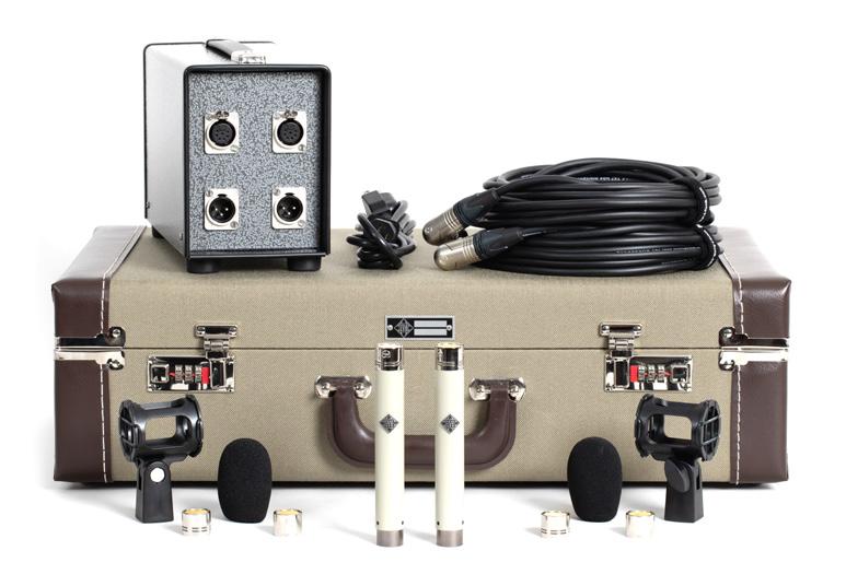
Known for their faithful recreations of classic gear, Warm Audio’s portfolio includes both large- and small-diaphragm capacitor mics, as well as ribbon models.

Key models: SDC: WA-84

LDC: WA-87, WA-CX12, WA-14SP, WA-CX24 stereo mic

Ribbon: WA-44, Fen-tone 1 2 3

Telefunken ELA M 260 Master Stereo Set

Warm Audio WA-CX24

Produce

Designed to support independent artists, producers, and collaborators at every stage of the music-making journey, SOS For Artists brings together all the tools needed to take your music from idea to release.

1. Sample Selection

Made Simple

Over 3 million royalty-free samples growing monthly.

2. Instruments & Synths

Includes a curated collection of high-quality plug-in instruments from brands like Spitfire, UJAM, Arturia, GForce, Sonuscore, and more.

3. Stem Extraction with AudioShake

An integrated stem-splitting plug-in allows you to isolate vocals, drums, bass, or instrumental parts.

4. Starter DAWs Included For newcomers, the subscription includes lite versions of Steinberg Cubase and Ableton Live

1. Mix & Effects Tools

The effects collection includes EQs, Compressors, Reverbs, Delays and Saturators from trusted names. Including Eventide, Arturia, Baby Audio, IK Multimedia, and Synchro Arts

2. Mastering — Fast, Intelligent

SOS For Artists includes access to the advanced AI mastering engine from LANDR.

Sign up and explore the features

Kickstart your creativity with 7,800 samples

Preview the LANDR Mastering tool

1. Global Digital Distribution

Distribute your music to over 150 platforms including Spotify, Apple Music, Tidal, Amazon, and Deezer. Or, if you use these platforms transfer all tracks to SOS For Artists without losing data.

2. Monetization & Royalty Splits

Retain 100% of your royalties or use the Royalty Split feature and divide the earnings with your collaborators.

Distribute or $12.99* per month or $19.99* per month

$1,000 worth of Tools inc 18 Plug-ins

1200 Sample Credits

Unlimited MP3 + up to 36 WAV masters

3. YouTube Integration

Link your official YouTube artist channel to keep distributed content and subscriber base in one place.

4. Promotion & Reporting

Promotion tools include Linktree-style landing pages and content creation tips to help boost visibility. Detailed royalty reporting shows trends, top countries, and top-performing platforms.

Preview Distribution $99 per year $199 per year ONLY ONLY

Unlimited Distribution

$2,000 worth of Tools inc 64 Plug-ins

2400 Sample Credits

Unlimited MP3, WAV + HD WAV masters

Unlimited Distribution

Buyer’s Guide

Stereo AccessoriesMiking

Mic stands, stereo bars and other accessories can be almost as important as microphones themselves.

Asimple stereo bar may be all you need to make coincident and near‑coincident stereo recordings — and many stereo microphone kits ship with a bar included. But for more complex setups, and when you need to be confident that your mics will stay exactly where you put them, a more professional solution might be called for. We round up some of the leading options.

AEA

AES’s SMS Stereo Bar features precisely spaced mounting holes for your mics, as well as angle markings for a range of coincident and near‑coincident techniques. You can even mount two ribbon or other figure 8 mics on it end‑to‑end, to create a Blumlein array.

W https://aearibbonmics.com

Ambient Recording

Ambient Recording make a range of high quality microphones and accessories, many of which are oriented at sound for picture and location recording. Their QAMS Stereo Bar is a highly flexible microphone mount for two mic stereo arrays such as X Y and A B, offering fully variable distances from 6 to 46.5 cm.

W https://ambient.de

Base 4 Stands

Base 4’s mic stands are suitable for any recording task, but their modular and lockable nature make them ideal for stereo arrays. The company even make a dedicated attachment for Blumlein recording.

W https://base4stands.com

Base 4 Stands Blumlein Attachment

Coles

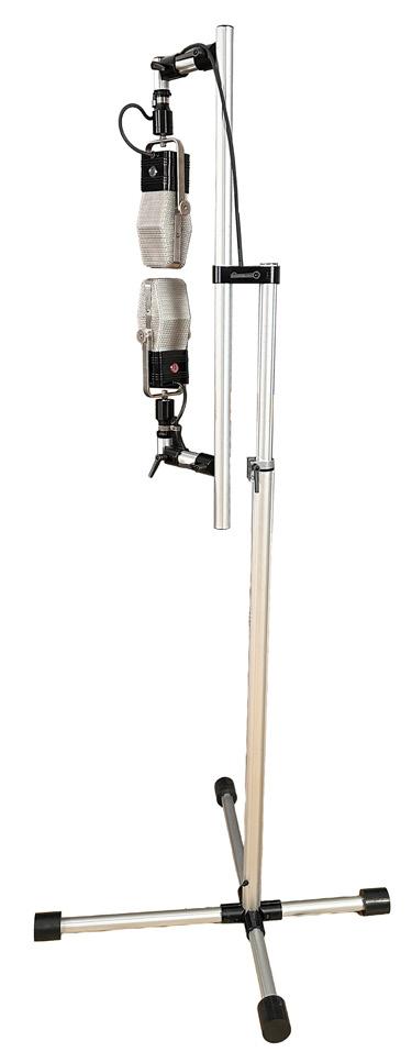
Amongst various other accessories, Coles make dedicated stereo mounts for their 4038 and 4030L ribbon microphones, allowing the mics to be rotated by up to 90 degrees.

W https://coleselectroacoustics.com/

Grace Design

Well known for their converters, preamps and processors, Grace also make the SpaceBar — an extremely well-engineered versatile stereo mounting bar, available in two sizes. It’s marked with measurements and angles, making it quick and easy to set up, and with everything easily and precisely repeatable.

W https://gracedesign.com

Gravity Stands

Gravity Stands, part of the German Adam Hall group, make stands and other accessories for a range of audio and media applications. Their MS STB 01 PRO is a stereo bar that allows for exact spacing of microphone mounts from 6 to 29 cm, ±90 degrees horizontal mic orientation, and up to ±90 degrees of tilt.

W www.gravitystands.com

JM Acoustic

Among JM’s range are compact mounts for X-Y and ORTF arrays, and 40mm Acoustic Pressure Equaliser spheres (APEs) — these are spherical acoustic baffles for use with omnidirectional microphones.

W www.jmacoustic.com

DPA

DPA produce Acoustic Pressure Equaliser (APE) spheres for their own 4006 mic, as well as a premium Stereo Boom mounting bar, and the S5 five-mic mount intended for Decca Tree and surround arrays.

W https://www.dpamicrophones.com

Latch Lake

Latch Lake’s microphone stands are known for their robustness and quality construction, and their micKing 2200 & 3300 models have realtively compact, heavy bases that make possible (when correctly counterbalanced) enormous height and horizontal reach.

W https://latchlakemusic.com

Manfrotto

Italian company Manfrotto make professional stands and other accessories for audio, photography, lighting and other applications. Their 154B Triple Microphone Support is a stereo bar with three

K&M

mic mount adaptors — one of which attaches to the stand — to be positioned freely along the cylindrical bar’s 65cm length.

W www.manfrotto.com

mikrofonschiene

mikrofonschiene manufacture a beautifully engineered modular mic bar system, with markings every 1 and 5 cm, that can be used for ORFT, A-B, M-S, Decca Tree and even surround arrays. Bar lengths of up to 2.4m can be created, but because they’re made from shorter modular sections, everything is easily transportable.

W https://mikrofonschiene.de

König & Meyer make a extensive range of mic stands and accessories, including the 23560 Microphone Bar, an extra-long bar (850 mm) with six elongated mounting slots, and knurled screws to allow for continuous adjustment.

W www.k-m.de

Royer

Famous for their ribbon microphones, Royer also make the FlexBar, a highly engineered and configurable two-mic holder suitable for a range of stereo miking arrays, including Blumlein.

W https://royerlabs.com

Rycote

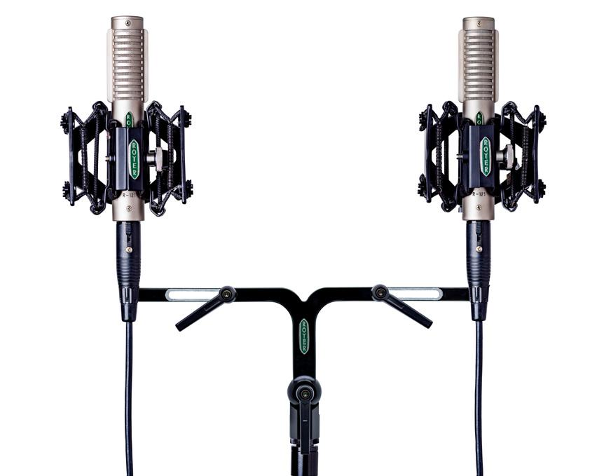
Rycote’s engineering-led shockmount designs are both innovative and highly effective. Included in their range is the InVision Stereo Pair Kit, which puts two of their mounts for small-diaphragm end-fire mics on a stereo mounting bar.

W https://rycote.com

Schoeps

Among Schoeps’ microphone accessories are the MAB 1000, a 1m stereo bar for two microphones in the A-B arrangement, but which also has a 10cm forward bar that allows the five-channel OCT surround technique to be supported. Markings every 2.5cm help to ensure precision, and the bar also features movable eyelets, to permit suspension from above. They also offer the KA 40, a 40mm Acoustic Pressure Equaliser (APE) sphere.

W https://schoeps.de

Sonodore

Sonodore make a range of mics, preamps and accessories. The latter category includes the AP-25, a 25mm APE intended for use with their own mics.

W www.rensheijnis.com

Superlux

The Superlux MS200 is a competitively priced professional steel overhead stand that’s robust enough for location work and can hold a serious combined weight of microphones without tipping or succumbing to boom-droop. The pole height can be set from

Shure

Shure’s pleasingly versatile A27M mic mount first saw service in 1980, and there’s a good reason it’s still available. By adjusting the relative angles of its two mounting studs, a wide variety of coincident, near-coincident and near-spaced stereo arrays can be configured. It can also accommodate mics of different diameters and lengths with far greater convenience than most conventional stereo bars.

W www.shure.com

165-350 cm, and the adjustable-length boom arm from 125-205 cm.

W www.superlux.com.tw

Triad-Orbit

Triad-Orbit make an extraordinarily versatile and comprehensive mic-stand system, with a wide and unusual range of accessories and attachments. Among them is the O2 Dual Arm Orbital Boom, comprising dual booms mounted on a proprietary ORBIT ball swivel mechanism, and a central swivel unit that provides an additional 45 degrees of left-right motion to the arms.

W www.triad-orbit.com

Ultimate Support

Colorado-based Ultimate Support make stands for a range of applications. The MC-125 is a large, sturdy studio boom stand with a large-diameter base and locking, rollerblade-style wheels that result in a low center of gravity to ensure stability. The long boom extends to 61 inches and an adjustable 5.75lb counterweight is included.

W www.ultimatesupport.com

Glossary

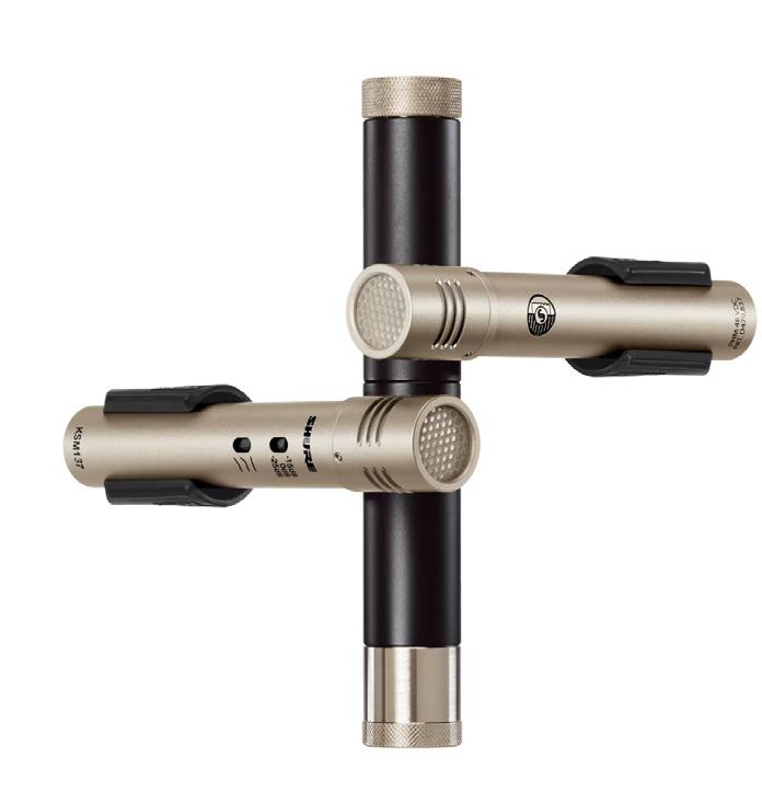
A B Stereo: A stereo microphone technique using two microphones spaced apart by at least 50cm. The microphones normally have omnidirectional polar patterns, but other polar patterns can be used. This format is known for capturing a good sense of spaciousness, depth and ambience, although spatial imaging tends to be relatively vague and is potentially unstable.

Acoustic Pressure Equaliser: see APE sphere.

Alan Blumlein: See Blumlein, Alan Dower

Angular Distortion: The differences between the relative angles of physical sound sources placed in front of a stereo microphone array and their representation as virtual sources on replay from stereo loudspeakers. Most stereo arrays tend to expand the relative angles of sources close to the centre but compress them for sources close to the edge (somewhat like a wide-angle lens).

APE Sphere (Acoustic Pressure Equaliser): A smooth spherical construction with a small-diaphragm omnidirectional microphone capsule mounted flush to the surface. APEs are typically 30-50 mm in diameter and serve to modify the frequency response and polar pattern through surface diffractions. These create an HF boost for on-axis sounds, and greater directivity at high frequencies, giving more forward focus and, when used in a spaced array, enhanced stereo imaging. The Decca Tree is famous for using Neumann M50 microphones in which the omni capsule is embedded within a 40mm APE.

Array: An arrangement of two or more microphones.

Auditory Cues: Elements of acoustic sound signals detected by the ears and brain that help to locate sound sources in the space around the listener, using inter-aural time differences (ITD), inter-aural level differences (ILD), and spectral anomalies due to comb-filtering caused by the pinnae and shoulders.

Baffle: An acoustic screen placed between microphones to replicate the sound-shadowing effect of the head between the ears. It serves to increase the level difference between the two microphones at high frequencies (depending on the baffle size) for an off-centre sound source.

Bass Tip up: See proximity effect

BBC: British Broadcasting Corporation, the UK’s public-service broadcaster.

Bell Laboratories: The historical research centre of the Bell Telephone Company in America, credited with (amongst many other inventions) the development of early stereo spaced-array microphone techniques concurrent with, but independent of, Blumlein’s work at EMI in the UK.

Binaural Hearing: The normal sense of hearing, which relies on the brain’s analysis of the small timing and level differences between sounds gathered by both ears.

Binaural Mic Technique: A stereo microphone technique intended for headphone listening, which aims to replicate the sound-gathering

characteristics of human ears. Typically, near-spaced omnidirectional microphones are separated by an acoustic baffle to imitate the basic structure of the human head. Commercial designs include Jecklin and Schneider discs, as well as dummy head systems.

Binaural Stereo: A form of stereo recording and playback system, whereby the binaural mic technique is used to create recordings intended specifically for playback over headphones, rather than loudspeakers — the aim is to present a realistic 3D immersive sound stage for the listener.

Blumlein, Alan Dower (1903‑1942): A pioneering British electronics engineer who worked initially for Standard Telephones and Cables (STC) and then the Columbia Graphophone Company, which later became EMI. Blumlein is credited as the inventor of stereophonic sound, and through his short career he was granted numerous patents for many inventions, including weighting networks for audio measurements, cable construction and transformer designs to improve the quality of long-distance telephone lines, a high-quality moving-coil disc-cutting head (for 78rpm records), the ultra-linear valve amplifier design, and the long-tailed pair differential amplifier. He also invented the coincident microphone array, baffled omni mic arrays, 45/45 stereo-groove vinyl records, Mid-Sides stereo, M-S matrixing and Stereo Shuffling techniques.

Blumlein was also involved in the early development of electronic television, including the waveform structure of 405-line black & white TV. It was this work that led to his secondment to the Telecommunications Research Establishment (TRE) during WWII to help develop H2S airborne radar, with its revolutionary cavity magnetron which generated a pulse microwave signal. Sadly, Blumlein was killed during an H2S test flight in

a Halifax bomber over Herefordshire in 1942, which suffered an engine fire and crashed. Modern audio-video technology owes a great deal to the genius of Alan Blumlein.

Blumlein Array: Two coincident microphones with figure-of-eight polar patterns arranged with a mutual angle of 80-100 degrees. Named after the British inventor Alan Dower Blumlein who used this configuration for much of his research into Intensity Stereo.

Blumlein Pair: See Blumlein Array.

Blumlein Pfanzagl Triple Array: A development of the Blumlein Array, named after its inventor Dr Edwin Pfanzagl-Cardone. This configuration adds a third, central figure-8 microphone facing directly forwards. This extra microphone’s output is typically blended 3-6 dB lower than the level from the left and right microphones to introduce more central focus to the sound stage, and may be accompanied by an acoustic shield to the rear.

Capsule: A reference to the acoustically sensitive part of a microphone containing the diaphragm(s).

Capsule Spacing: The distance between the centres of the diaphragms of the microphones in a stereo array.

Cardioid: A microphone polar pattern in which the sensitivity at the sides (90 and 270 degrees) is around 6dB lower than at the front (0 degrees), with a deep null at the rear (180 degrees). Some sound energy is allowed to reach the rear of the diaphragm after a short delay, effectively combining 50-percent pressure and 50-percent velocity operation. The velocity component means the microphone has a modest amount of proximity effect.

Coincident: The placement of two or more microphone capsules as closely

together as possible, such that they capture sounds from any direction at the same instant. In practice, since they can’t occupy precisely the same point in space, capsules are normally mounted directly above each other — this ensures coincidence in the horizontal plane, accepting a small inherent spacing in the vertical plane.

Coincident Microphones: A pair of microphones arranged with their capsules coincident to create a recording with only level differences between the two channels. Often also referred to as the X-Y format, and used with directional microphones (cardioid, hypercardioid, figure-8 etc). The Mid-Sides array is also a coincident format.

Combination Stereo Array:

A complex multi-mic stereo array typically combining two or more conventional stereo arrays mounted in the same plane. The OCCO array and Faulkner phased array are examples of combination arrays, where a near-coincident array is combined with a spaced-omni array with the aim of blending the spatial imaging accuracy of the former with the spaciousness and low-frequency extension of the latter.

Comb-filtering: When two similar signals are summed together with a small timing difference between them, the relative phase-shifts between their similar frequency components cause peaks and troughs in the frequency response, which loosely resemble the teeth of a hair comb, hence the name (also known as an interference pattern). The sound of comb-filtering is noticeably coloured and possibly even ‘phasey’ in character.

Correlation: An expression of the degree of similarity between signals conveyed over two channels. A dual-mono signal would have full correlation, whereas two spaced-omni microphones would capture signals with very little

correlation. Normal stereo material with a wide sound stage has a significant degree of decorrelation between channels.

Correllation Meter: See phase meter

Critical Distance: Denoted as Dc, this is the distance from a directional sound source at which the sound pressure level of the direct sound exactly equals that of the reverberant sound. Dc is dependent on the geometry and absorption characteristics of the space in which the soundwaves propagate. A highly reverberant space has a relatively short Dc, whereas a dry-sounding room has a long Dc. Critical distance is important in determining where to locate microphones to achieve a desired perspective.

Crossed Pair: See coincident microphones and X-Y stereo.

Crossfeed Matrix: A technology often employed in headphone monitoring to recreate the acoustic crosstalk between ears which naturally occurs with loudspeaker listening, but which is normally excluded by headphones. A portion of the signal from each channel is fed into the opposite channel with equalisation and a short delay.

Crosstalk: Signal bleed from one channel into another. Depending on the polarity of the crosstalk, it can either reduce or increase the stereo width. Although usually deemed undesirable, it can also be employed deliberately for creative purposes (see crossfeed matrix).

Curtain of Sound: An approach to capturing and reproducing stereophonic sound developed by Dr Harvey Fletcher (of Bell Labs in America) in the early 1930s. A multiplicity of microphones arrayed in front of a large ensemble sample the audio wavefront at different points in space. Each microphone is

connected to a corresponding loudspeaker in front of the audience to recreate the same wavefronts. Although effective, this technique was deemed highly impractical at the time, and it evolved through simplification into various spaced-omni microphone techniques.

DAW (Digital Audio Workstation):

A computer-based audio recording, processing and mixing tool.

DC Offset: A fault condition whereby the AC audio signal is offset by a DC voltage. Historically caused by bad digital converters or signal processing, but very rare today. It can cause asymmetrical clipping and loud clicks on editing or switching the affected signal. (Not to be confused with perfectly normal and common asymmetrical audio signals.)

Decca Tree: A stereo microphone technique developed in the early 1950s by Decca Records engineers Roy Wallace and Arthur Haddy. A common implementation uses a pair of omnidirectional microphones spaced around two metres apart, with a third in the centre and 1.5 metres forward, although the precise dimensions are typically varied to suit the size of recording ensemble. All three microphones use APEs and the outer pair are angled outwards. (The Neumann M50 microphone is widely associated with this technique.) For large orchestral settings, an additional pair of omni outriggers are also employed located roughly two thirds of the way from conductor to outer edge of the orchestra, along with a sixth mic to accent the double basses.

Decorrelation: Dissimilarities between two audio channels, particularly in their phase relationships (see also correlation).

Diaphragm: The front element of a microphone which moves in response to passing soundwaves.

DIN: An acronym for a German standards organisation founded in 1917: Deutsches Institut für Normung. Amongst many audio standards created by this organisation, the DIN stereo microphone array comprises a pair of near-spaced cardioid microphones with capsules spaced 20cm apart at a mutual angle of 90 degrees. The resulting SRA is 101 degrees. This technique captures both time and level differences between channels, and is comparable to techniques such as ORTF, RAI, EBS, NOS, and others.

Directionality: The ability of a microphone to reject or reduce sounds from certain directions due to its polar pattern. (See cardioid, hypercardioid, figure-8.)

Directivity: See directionality

DMS: See double Mid-Sides array

Double Mid-Sides Array: An extension of the Mid-Sides microphone concept, in which a second Mid microphone is added to the array, but facing directly backwards. This system requires only three audio channels, but can be decoded to create five channels — the shared Sides mic is used with the rearward Mid mic to generate rear left and rear right signals suitable for surround-sound applications. Sometimes referred to as the DMS format, and employed where a compact surround-sound mic array is required.

Dual-mono: Identical audio content carried in both the left and right channels of a stereo system (ie. panned centre), resulting in a phantom centre sound image.

Dummy Head: A stereo microphone device resembling a human head, often with a partial torso, designed to closely emulate the acoustic properties of the human head, with microphones located where the ears would normally be. The output is a binaural signal.

Eardrum: The diaphragm at the inner end of the ear canal which responds to passing soundwaves, coupling the energy through to the impedance-converting bones of the middle ear and on to the cochlear or inner ear for conversion into brain impulses.

EBS: An eponymously named near-spaced stereo microphone system developed by Eberhard Sengpiel (1940-2014). It comprises a pair of cardioid microphones with capsules spaced 25cm apart at a mutual angle of 90 degrees. The resulting SRA is 90 degrees. This technique captures both time and level differences between channels, and is comparable to similar techniques such as ORTF, RAI, DIN, NOS and others.

EMI: Electric & Music Industries, a record label which evolved from the Columbia Graphophone Company in 1931. Its research department employed Alan Blumlein and was instrumental in the early development of stereophonic sound.

Equilateral Triangle: A triangle with three equal-length sides at angles of 60 degrees to each other. Blumlein recommended that stereo loudspeakers should be configured with loudspeakers at two corners, facing the listener at the third.

Fantasound: A set of pioneering technologies developed by Walt Disney Studios in the late 1930s for the film Fantasia. It was the first commercial surround-sound system, which pioneered the use of pan pots for sound positioning, multitrack recording, overdubbing, click tracks for synchronisation, control tracks for automatic gain control, and more.

Faulkner Phased Array: A stereo microphone technique made popular by the esteemed British recording engineer Tony Faulkner. Similar in appearance to the OCCO array, it uses a pair of near-spaced cardioid

microphones flanked by a pair of spaced omnidirectional mics. The cardioid pair has a capsule spacing of around 41cm while the omnis are spaced at 67cm. Both pairs have 90‑degree mutual angles.

Faulkner explains the concept as being similar to steerable radio frequency aerial arrays, whereby the reception beam focus is orientated by manipulating the relative phases of signals from each aerial element — although that’s not how the microphones are actually used in this array, as there is no direct phase manipulation.

Another stereo mic array associated with Faulkner, and sometimes also called a ‘phased array’, employs a pair of figure 8 microphones spaced 20cm apart both facing directly forward (mutual angle 0 degrees). This is essentially a spaced omni array but designed to minimise unwanted side reflections in acoustically difficult venues by replacing the omnidirectional microphones with figure of eight types.

Faulkner, Tony: British recording engineer and producer associated with classical and choral recordings. Also known for two stereo microphone arrays.

Figure 8: Also written as fig 8, figure of‑eight, or figure of 8. A microphone polar pattern in which the sensitivity at the rear (180 degrees) is the same as the front (0 degrees), but with opposite polarity. There are deep nulls at both sides (90 and 270 degrees), such that when plotted out in two dimensions it resembles the digit ‘8’. The figure 8 microphone uses 100‑percent velocity (pressure gradient) operation, which means it also has a very strong proximity effect

Fletcher, Dr Harvey (1884‑1981): An American physicist who worked for Bell Laboratories on the development of stereophonic sound, amongst other things,

in the early 1930s. Though a contemporary of Alan Blumlein, he was developing stereo techniques entirely independently.

Frequency: A count of the number of vibrations or cycles of a sound waveform in one second, denoted in Hertz (Hz). In musical terms frequency is described as pitch: a high frequency is a high pitch, and vice versa. Human hearing nominally spans the range 20Hz‑20kHz.

Gerzon Array: A near coincident stereo microphone array described in detail by British audio engineer Michael Gerzon but also credited to Tony Faulkner. It comprises a pair of cardioid microphones with capsules spaced 5cm apart at a mutual angle of 120 degrees. The resulting SRA is 130 degrees. This technique captures both time and level differences between channels, and is comparable to similar techniques such as ORTF, RAI, DIN, NOS and others, but with a noticeably smaller spacing and wider mutual angle. It is often used with a Stereo Shuffling process to enhance the sense of spaciousness at low frequencies.

Gerzon, Michael: A British mathematician and recording engineer best known for his work on Ambisonics and digital audio processing (1945‑1996). (See Gerzon array.)

Goniometer: A stereo audio vectorscope that displays the stereo sound image as a Lissajous figure to assess the correlation and stereo width between two channels, as revealed by the phase and amplitude relationships between the channels. The two audio channels are plotted on diagonal axes, such that a left only signal is shown as a diagonal line from top left to bottom right, while a right only signal runs from top right to bottom left. An identical signal on both channels (dual mono) results in a thin vertical line, while identical

signals in opposite polarity create a thin horizontal line. Normal stereo creates the appearance of a circular tangled ‘ball of string’.

Head‑related Transfer Functions (HRTFs). Parameters that describe a unique set of acoustic filters, created by sound reflections from an individual’s head, shoulders and pinnae, which modify the soundwaves entering the ear canal. These unique characteristics are learned to allow the brain to locate sound sources in the 3D space around the listener. Perceiving accurate sound placement from a binaural audio source relies very heavily on the material being processed accurately with an individual’s personal HRTFs.

Hole‑in‑the‑middle: An effect whereby the stereo sound appears to ‘puddle’ near the two loudspeakers, without creating a continuous sound stage between them. It commonly occurs if microphones in a stereo array are spaced too far apart.

HRTFs: See Head‑related Transfer Functions

Hybrid Array: A stereo microphone array designed to combine the most attractive qualities associated with both spaced omni (A B) and coincident (X Y) arrays. Inter channel level differences are captured by angling directional microphones outwards, and inter channel time differences are obtained by spacing the microphone capsules apart. In practice, some of the imaging accuracy associated with coincident techniques is sacrificed for the much greater sense of spaciousness associated with spaced omni techniques. Popular hybrid arrays include ORTF, NOS, DIN, EBS, RAI and Gerzon

Hypercardioid: A microphone polar pattern in which the sensitivity at the sides (90 and 270 degrees) is around 12dB lower than at the front (0 degrees), and there’s an

opposite-polarity rear lobe which is between 6 and 10 dB less sensitive at 180 degrees than the front (0 degrees). This rear lobe creates two deep rejection nulls at about 110 and 250 degrees. This polar pattern is derived from about 25-percent pressure operation and 75-percent velocity operation, so it has a strong proximity effect.

ILD: See inter-aural level differences

Intensity Stereo: The name given by Alan Blumlein to a stereo signal comprising only amplitude differences between the two channels. It can be created by using a pan pot in a mixing console, or with coincident (X-Y) microphones

Inter-aural Level Difference (ILD):

The difference in loudness or intensity of a soundwave reaching the left and right ears. In real life this is caused by diffraction of sound around the head at high frequencies (above about 700Hz), causing a ‘sound shadow’ for the more distant ear. The brain uses the inter-aural level difference as a means of identifying the location of a sound source, which will be louder on the side of the closer ear. See also inter-aural time difference (ITD).

Inter-aural Time Difference (ITD):

The difference in the arrival time of a soundwave reaching the left and right ears. In real life this is caused by the extra distance the soundwave has to travel around the head, resulting in a detectable phase-shift for frequencies below about 700Hz. The brain uses the inter-aural time difference as a means of identifying the location of a sound source, which will be earlier on the side of the closer ear. See also inter-aural level difference (ITD).

Interference Pattern: See comb-filtering

ITD: See inter-aural time difference

Jecklin Disc: A stereo microphone

device used primarily for capturing binaural stereo. Designed by Jürg Jecklin in the early 1980s and referred to as the OSS technique, as a development of Alan Blumlein’s early experiments with spaced omnidirectional microphones, it comprises a circular baffle of 30cm diameter with acoustic absorption material on both surfaces to approximate the acoustic characteristics of the human head. Omnidirectional microphones are placed on either side with a roughly 16.5cm spacing and angled outwards at 20 degrees. Jecklin revised the design in 2003 to have a larger 35cm diameter disc with wider 36cm mic spacing. The Schneider Disc is very similar but features additional sphere of acoustic absorption at the centre of the baffle.

Large-diaphragm Microphone: Usually refers to a capacitor (condenser) microphone with a capsule diaphragm of around one inch in diameter. The large-diameter diaphragm allows very low self-noise performance, but also compromises high-frequency extension and increases directivity at higher frequencies, essentially narrowing the intended polar pattern. (See also small-diaphragm microphone).

Linear-phase EQ: A form of digital equaliser that adjusts the amplitude at different frequencies without introducing phase-shifts, something that cannot be practically achieved in the analogue domain. Also known as a non-causal filter, this type of EQ inherently introduces latency to the signal path.

Lissajous Figure: A two-dimensional visual pattern produced by the interaction of two independent signals, each controlling the amplitude of one display axis. (See also goniometer and vectorscope.)

Lobes: In the context of microphone polar patterns, a lobe is a region around the microphone sensitive to sound. A figure-8

microphone has front and rear lobes of equal sensitivity, whereas the rear lobe of a hypercardioid microphone is 6-10 dB less sensitive than the front.

M3: A reference to the attenuation applied to a summed-mono signal to maintain electrical headroom and to give a perceived acoustic volume consistent with the stereo source. M3 uses a 3dB attenuation ((A+B)-3dB) and is most appropriate where the stereo source comprises largely decorrelated signals (ie. normal stereo). (See also M6.)

M6: A reference to the attenuation applied to a summed-mono signal to maintain electrical headroom and to give equivalent metering levels with the stereo source. M6 uses a 6dB attenuation ((A+B)-6dB) and is most appropriate where the stereo source has largely correlated signals (ie. dual-mono). (See also M3.)

Matrix: See Mid-Sides matrix

Mid-Sides Array: A coincident microphone array which captures the stereo field directly in its Mid and Sides components, requiring decoding through a matrix before auditioning as normal left-right stereo. The Mid microphone faces directly forwards and can have any desired polar pattern. The Sides microphone is always a figure-8 type facing 90 degrees left, with the left lobe having the same polarity as the front of the Mid microphone. The relative balance of the Mid and Sides components determines the stereo recording angle

Mid-Sides Matrix: Sum and difference circuitry to convert between conventional left-right stereo and the Mid-Sides format. It can be achieved through passive transformers or active electronics. The required processes are defined by a simple formula:

M = (L+R) and S = (L–R) Or: L=(M+S) and R=(M–S)

Mid Sides Stereo: An alternative stereo format in which the Mid channel encodes information across the entire stereo field, weighted towards the centre. The Sides channel also encodes information across the entire stereo field, weighted towards both edges, but completely excluding information from the centre.

Monaural: Listening with only one ear, or conveying audio information on a single channel.

M S: See Mid Sides Stereo

Mutual Angle: The angle measured between the primary sensitivity axes of two microphone capsules. The mutual angle is significant in determining the stereo recording angle (SRA) of a coincident or near coincident stereo microphone array.

Near‑coincident Microphones:

A stereo microphone array using directional microphones angled apart in the same way as a coincident array, but with the capsules also spaced apart by a small distance (less than 50cm) to capture small inter channel timing differences in addition to the inter channel level differences.

Near spaced Microphones: See Near coincident Microphones

Neumann M50: An omnidirectional capacitor microphone introduced by Neumann in 1950 and the first to mount a small diaphragm capsule flush within a 40mm Acoustic Pressure Equalisation sphere (APE). The APE boosts the high frequency response on axis to give a flat frequency response when placed in the diffuse field, effectively compensating for the HF losses associated with distant placement. The APE also increases directivity (narrowing the polar pattern) at high frequencies, which is crucial when used in the Decca Tree microphone array.

NOS Array: A near coincident stereo microphone array conceived by the Dutch broadcaster Nederlandse Omroep Stichting (NOS) in the early 1960s. It comprises a pair of cardioid microphones with capsules spaced 30cm apart at a mutual angle of 90 degrees. The resulting SRA is 81 degrees. This technique captures both time and level differences between channels, and is comparable to similar techniques such as ORTF, RAI, DIN, EBS and others.

OCCO Array: Also referred to as the Optimal Cardioid Capsule Configuration, this is a combination stereo array that typically employs both a near coincident array and a spaced omni array in the same system, with the two pairs of microphones being blended to achieve the desired level of imaging precision, spaciousness and LF extension.

Omnidirectional: A microphone polar pattern in which the sensitivity to sound is constant at all angles of incidence. It employs only pressure operation and has no proximity effect at all. Most omnidirectional microphones have considerably more low frequency extension than any directional (velocity operation) microphone.

Optimal Cardioid Capsule Configuration: See OCCO array

Optimal Stereo Signal (OSS): The name given to a binaural stereo microphone system developed by Jürg Jecklin but better known as the Jecklin Disc. The Optimal Stereo Signal is often abbreviated to OSS.

ORTF Array: A near coincident stereo microphone array conceived by the French broadcaster Office de Radiodiffusion Télévision Française (ORTF) in the early 1960s. It comprises a pair of cardioid microphones with capsules spaced 17cm apart at a mutual angle of 110 degrees. The resulting SRA is 96 degrees. This technique

captures both time and level differences between channels, and is comparable to techniques such as NOS, RAI, DIN, EBS, and others.

OSS Technique: See Optimal Stereo Signal

Panned: The act of using a pan pot to position a monaural sound source within a stereo sound stage.

Pan Pot: The pan pot (panoramic potentiometer) was conceived during the development of Fantasound, and is an electrical control used to split a monaural signal to feed the left and right stereo outputs in varying proportions. This creates inter‑channel level differences between the left and right channels which, when auditioned over loudspeakers, create the impression of a virtual sound source at any desired location between the two speakers, in a similar way to a coincident microphone array.

Periodic Signals: A signal that repeats its waveform pattern exactly after a fixed time period. The obvious examples are sine waves and square waves. Signals that don’t repeat, such as transients, are aperiodic

Perspective: The perceived distance of a sound source, determined by the relative balance of direct and reflected sound. A close perspective implies more direct than reflected sound, whereas a distant perspective suggests a more reverberant sound with little direct content. When recording, the perspective is determined by both the distance of the microphones from the sound sources and the acoustic character of the recording venue (see also critical distance).

Phantom Centre: The perceived location, mid way between two loudspeakers, of a sound source when both left and right channels carry identical audio signals.

Phase‑shift: The displacement in time of a periodic signal. Phase is

the angular difference between two waves of the same frequency. A phase shift of 180 degrees appears to invert the signal.

Phase Meter: See phase correlation meter

Phase Correlation Meter: An audio meter designed to indicate the phase relationships (correlation) between left and right stereo audio signals. Various meter formats are used, but most are scaled from +1 to -1, with zero at the centre. Full correlation (ie. dual-mono) is shown as +1, while opposite polarity is shown as -1. Fully wide stereo material (decorrelated) would register around 0. Signals indicated anywhere between +1 and 0 are considered mono-compatible. Dips below 0 towards -1 suggest a listener of the summed mono signal will hear coloured or severely attenuated audio.

Phased Array:

See Faulkner Phased Array

Pinnae: The visible outer part of the human ear which helps to guide sound into the ear canal, creating auditory cues in the process through shadowing and interference effects for sounds from different directions at high frequencies.

Polar Pattern: A two-dimensional plot showing a microphone’s sensitivity to sound arriving from different directions. See omnidirectional, cardioid, hypercardioid and figure-8

PPM: Peak Program Meter. An analogue sound level meter designed to register quasi-peak sound levels, invented in the 1930s and widely used by European broadcasters. Several variations on the theme exist (EBU, DIN, BBC, Nordic) with different scales but similar dynamic specifications.

Pressure Operation: The simplest form of microphone capsule in which a diaphragm encloses a chamber of atmospheric air. A passing

soundwave causes the diaphragm to move in and out as compressions and rarefactions pass, effectively comparing the air pressure variations of the soundwave with the static ambient air pressure held within the chamber. The diaphragm’s movement is not dependent on the direction of soundwaves, merely their passing, so the polar pattern is omnidirectional. There is also no proximity effect, and the system remains sensitive to very low frequencies.

Pressure Gradient Operation: See velocity operation

Proximity Effect: All directional microphones which involve some proportion of velocity operation suffer a side-effect in which the sensitivity to low frequencies increases significantly as a sound source approaches the microphone capsule. Also known as ‘bass tip-up’.

RAI: A near-coincident stereo microphone array conceived by the Italian broadcaster Radio Audizioni Italiane (RAI) in the early 1960s. It comprises a pair of cardioid microphones with capsules spaced 21cm apart at a mutual angle of 100 degrees. The resulting SRA is 93 degrees. This technique captures both time and level differences between channels, and is comparable to techniques such as NOS, ORTF, DIN, EBS, and others.

Schneider Disc: A stereo microphone device used primarily for capturing binaural stereo, and a variation on the OSS technique. Similar to the Jecklin Disc, the Schneider Disc comprises a circular baffle of 30cm diameter with acoustic absorption material on both surfaces supplemented with a 12cm foam-covered sphere at the centre of the disc to better approximate the acoustic characteristics of the human head. Omnidirectional microphones are placed on either side with a roughly 16.5cm spacing and angled outwards at 20 degrees.

Sengpiel Visualisation Tool: Created by recording engineer Eberhard Sengpiel (1940-2014), this visualisation tool takes the form of an interactive web page that calculates the stereo recording angle (SRA), angular distortion and relative proportions of ILD and ITD generated by different stereo microphone configurations.

Separated Arrays: A complex multi-mic stereo array typically combining two or more conventional stereo arrays mounted at different distances from the source but blended together to form a single stereo signal. For example, a small ensemble might be captured using a close spaced-omni array blended with a more distant ORTF array.

Shuffler: See shuffling

Shuffling: A signal-processing technique first conceived by Alan Blumlein to correct for spatial imaging anomalies inherent in stereo microphone arrays and loudspeaker monitoring. All shuffling processes involve frequency-dependent adjustments to the width of a stereo signal at different frequencies.

Sine Wave: A simple oscillation creating a periodic signal at a single frequency, with an amplitude described by the trigonometric sine function.

Small-diaphragm Mic: Usually refers to a capacitor (condenser) microphone with a capsule diaphragm of less than half an inch in diameter. The modest diaphragm size allows good high-frequency extension and maintains a reasonably accurate polar pattern at all frequencies. See also large-diaphragm microphone

Sound Shadow: The area behind an acoustic baffle on the opposite side from the sound source where the sound level is greatly reduced due to sound diffracting around the baffle.

Spaced Array: See spaced omnis

Spaced Omnis: A stereo recording technique using omnidirectional microphones with capsules typically spaced more than 50cm apart, which causes them to capture mainly inter-channel timing differences. (See A-B stereo.)

Spaciousness: The implied sense of space, or presence in a large acoustic volume, when listening to stereo audio. It is largely created through low-frequency decorrelation

Spatial Distortion: The difference between the angles between physical sound sources relative to a stereo microphone array, and the angles of the corresponding virtual images created between stereo loudspeakers.

SRA: See stereo recording angle.

Stereo Bar: Mounting hardware designed to fix atop a microphone stand and support multiple microphones in variety of configurations. For example, Manfrotto’s 154b and Grace Designs’ Spacebar.

Stereo Imaging: The perception of virtual sound sources spread between stereo loudspeakers.

Stereo Microphone Array: Typically, a pair of microphones arranged to capture the relative positions of sound sources laid out in front of the mics, encoding that information across two audio channels using inter-channel level and/or inter-channel timing differences.

Stereo Recording Angle (SRA): The angle in front of a stereo microphone array within which physical sound sources are captured and subsequently reproduced as virtual sources in a stereo sound stage between stereo loudspeakers.

Stereo Shuffling: See shuffling

Stereo Sound Stage: The portrayal of virtual sound sources between stereo loudspeakers.

Stereo Spread: See stereo sound stage.

Stereo Width: The perceived portion of total width between stereo loudspeakers occupied by one or more virtual sound sources.

Stereophonic: The name given to two-channel audio by Alan Blumlein.

Stereophonic Zoom: A graphical method determining the stereo recording angle and spatial distortion for different microphone capsule spacing, mutual angle, and polar pattern, developed by Michael Williams.

Stereosonic Shuffler: A specific form of shuffler circuit designed by EMI in the 1950s to correct for the unwanted widening of high frequencies inherent in stereo loudspeaker listening and the Blumlein array

Stereo Vectorscope: See goniometer

Sum & Difference: The mathematical process of adding and subtracting two audio channels to convert between the left-right and Mid-Sides formats (and vice versa). See Mid-Sides matrix

Tony Faulkner: See Faulkner, Tony

Transients: Brief aperiodic signals, normally found at the starts of acoustic sounds, and typically louder than the sustained body of sound.

Twin-twin PPM: A type of stereo analogue audio level meter developed by the BBC. Two Peak Programme Meters are placed side by side, each with dual-concentric needles. One shows the left and right signals on red/green needles, while the other shows the equivalent Mid and Sides signals on white and yellow needles, respectively.

Vectorscope: See goniometer

Velocity Operation: A capsule design in which the diaphragm is suspended in open air to detect the difference in relative air pressure on each side of the diaphragm. This design is most sensitive to soundwaves arriving from directly in front or from behind (the latter with opposite polarity). If the sound source moves above or below the diaphragm the difference in air pressure on each side reduces so the capsule becomes progressively less sensitive, giving a figure-8 polar pattern. The diaphragm mounting is designed to be very compliant at low frequencies to maximise the sensitivity to very small pressure differences. This creates a very strong proximity effect

Virtual Sound source: The perception of a discrete sound source recreated between stereo loudspeakers.

Wavelength: The distance over which a periodic waveform repeats, ie. the distance between wave peaks or troughs. Wavelength is longer at lower frequency, and vice versa, the two being related by the speed of sound:

λ = v/f

where λ is the wavelength, f is the frequency, and v is the speed of sound.

Wide-spaced microphones: A spaced omni microphone array but with wider than normal spacing (typically two metres or more) to maximise decorrelation. (See spaced array.)

Williams, Michael: A British audio engineer best known for his published articles and books studying the physics and practicalities of stereo and multi-channel microphone arrays.

X-Y Stereo: See coincident microphones

THE WORLD’S BEST RECORDING TECHNOLOGY MAGAZINE

Sound On Sound now offers our Full Issue PDF. This complete digital replica of the Print magazine includes all articles and adverts published in that edition. Buy and download instantly - no shipping costs!

Only £3.99 / US$5.99 each edition (or FREE with all Digital subscriptions).

PDF can be viewed on your desktop, smartphone or tablet.

Stereo Miking

FI-PDFs remain in your MY ACCOUNT > DOWNLOADS library after purchase and can be re-downloaded at any time in the future.

Get your FREE PDF today at: https://sosm.ag/FreePDF