South African Journal of Science Vol. 121 No. 11/12
Status of wild rooibos and its ecotypes
Stone tools and knowledge sharing in the Stone Age
Research software: Key but neglected in digital research
EDITOR-IN-CHIEF
Leslie Swartz
Academy of Science of South Africa
EDITOR-IN-CHIEF MENTEE
Doniwen Pietersen
College of Education, Unisa, South Africa
MANAGING EDITOR
Linda Fick
Academy of Science of South Africa
ONLINE PUBLISHING SYSTEMS ADMINISTRATOR
Nadia Grobler
Academy of Science of South Africa
ONLINE PUBLISHING ADMINISTRATOR
Phumlani Mncwango Academy of Science of South Africa
ASSOCIATE EDITORS
Pascal Bessong
HIV/AIDS & Global Health Research Programme, University of Venda, South Africa
Chrissie Boughey
Centre for Postgraduate Studies, Rhodes University, South Africa
Teresa Coutinho
Department of Microbiology and Plant Pathology, University of Pretoria, South Africa
Thywill Dzogbewu
Department of Mechanical and Mechatronics Engineering, Central University of Technology, South Africa
Jemma Finch
School of Agricultural, Earth and Environmental Sciences, University of KwaZulu-Natal, South Africa
Jennifer Fitchett
School of Geography, Archaeology and Environmental Studies, University of the Witwatersrand, South Africa
Vusi Gumede
DVC: Teaching & Learning, Durban University of Technology, South Africa
Stefan Lotz
South African National Space Agency
Philani Mashazi Department of Chemistry, Rhodes University, South Africa
Sydney Moyo Department of Biological Sciences, Louisiana State University, LA, USA
ASSOCIATE EDITOR
MENTEES
Nkosinathi Madondo Academic Literacy and Language Unit, Mangosuthu University of Technology, South Africa
Shane Redelinghuys
National Institute for Communicable Diseases, South Africa
South African Journal of Science
Obituary
‘Bob’ Alexander Pullen (1939–2025): A legacy of institutional
Medical research, evidence and politics: An insightful history of the South African Medical Research Council, 1969–2022
Perspectives
Responsible
Research
A key (neglected) component of the digital research infrastructure ecosystem
Anelda van der Walt, Kim Martin, Sumir Panji, Angelique Trusler, Mattia Vaccari, Peter van Heusden
EDITORIAL ADVISORY BOARD
Saul Dubow
Smuts Professor of Commonwealth History, University of Cambridge, UK
Pumla Gobodo-Madikizela Trauma Studies in Historical Trauma and Transformation, Stellenbosch University, South Africa
David Lokhat
Discipline of Chemical Engineering, University of KwaZulu-Natal, South Africa
Robert Morrell School of Education, University of Cape Town, South Africa
Pilate Moyo Department of Civil Engineering, University of Cape Town, South Africa
Catherine Ngila African Foundation for Women & Youth in Education, Sciences, Technology and Innovation, Nairobi, Kenya
Daya Reddy
Applied Mathematics, University of Cape Town, South Africa
Linda Richter
DST-NRF Centre of Excellence in Human Development University of the Witwatersrand, South Africa
Brigitte Senut
Natural History Museum, Paris, France
Benjamin Smith Centre for Rock Art Research and Management, University of Western Australia, Perth, Australia
Himla Soodyall Academy of Science of South Africa, South Africa
Lyn Wadley
School of Geography, Archaeology and Environmental Studies, University of the Witwatersrand, South Africa
Published by the Academy of Science of South Africa (www.assaf.org.za) with financial assistance from the Department of Science, Technology & Innovation
Design and layout
Lumina Datamatics
Correspondence and enquiries
sajs@assaf.org.za
Copyright All articles are published under a Creative Commons Attribution Licence. Copyright is retained by the authors.
Disclaimer
The publisher and editors accept no responsibility for statements made by the authors.
Submissions
Submissions should be made at www.sajs.co.za
On the cover
Invited Commentary
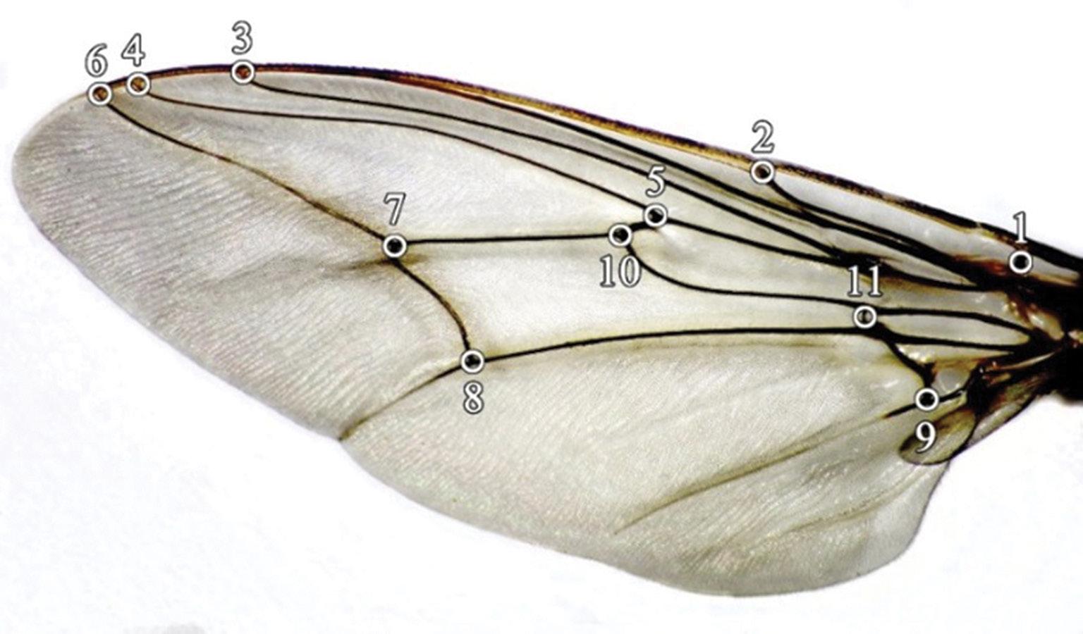
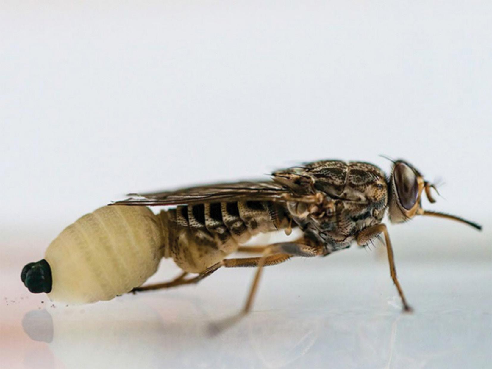
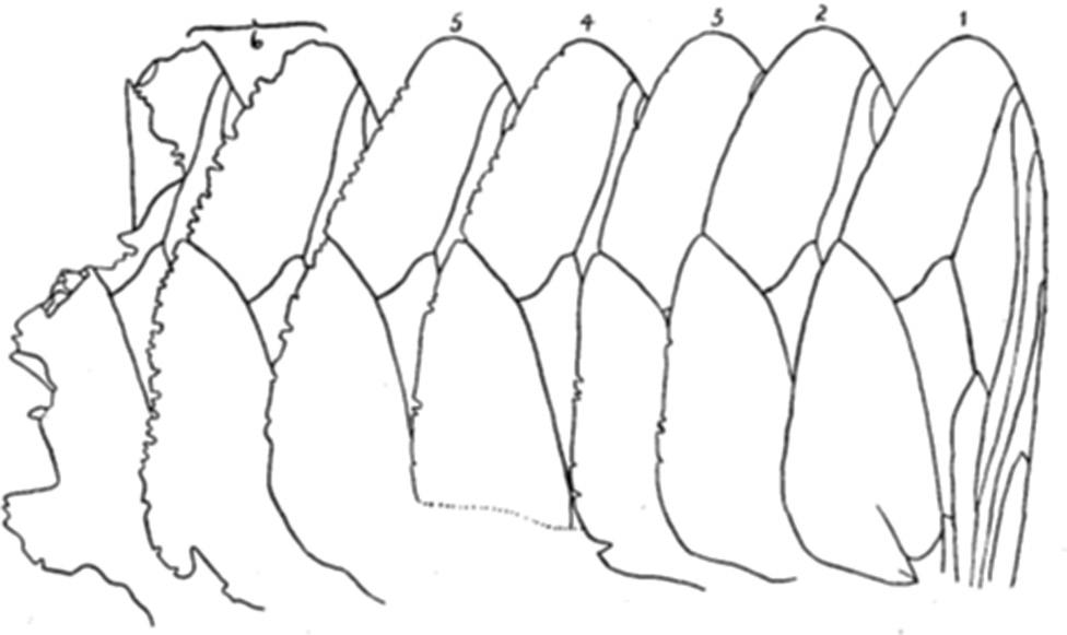
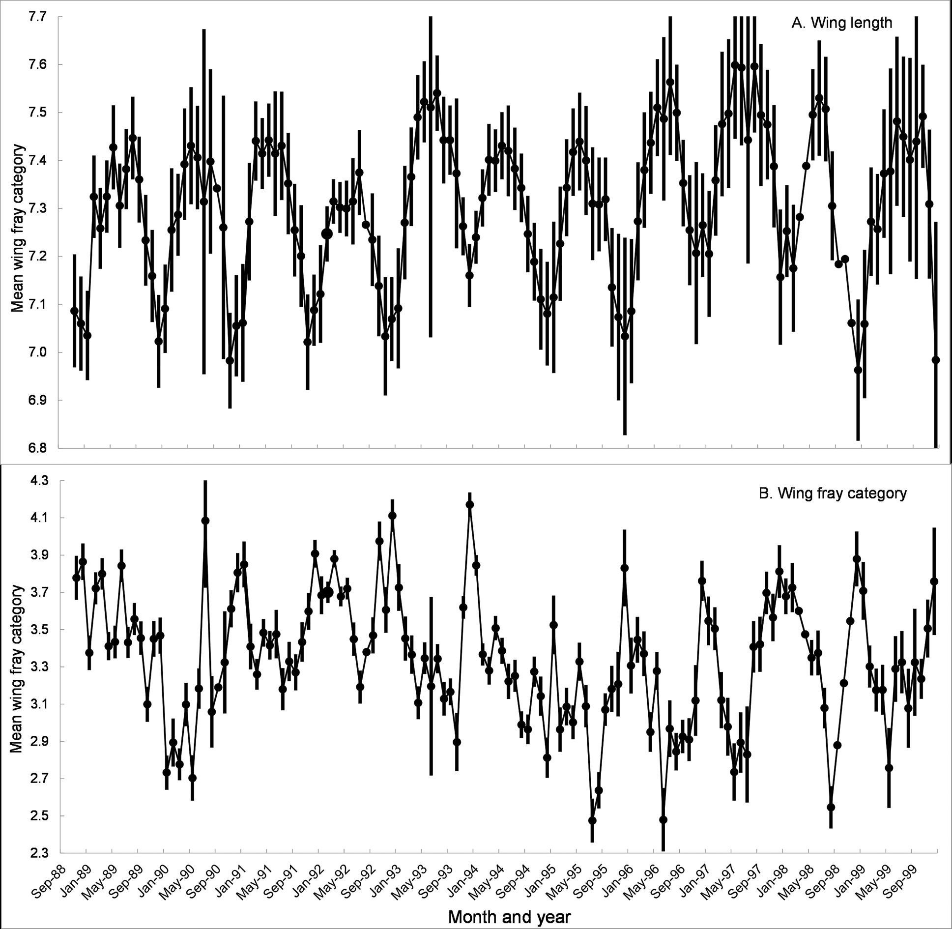
Written on the wings: Morphometrics, mortality and more John W. Hargrove, Pietro Landi, Willie Brink
Commentaries
Sounds like non-ideal Mars atmospheric data
Robin E. Kroon
The hidden cost of open access: Artificial intelligence, paywalls and the risk of knowledge inequity
Brenda D. Wingfield, Beverley J. Wingfield
Australopithecus at Sterkfontein, South Africa: Consumer of mammalian meat?
Francis Thackeray
Review Articles
Middle Stone Age social connectivity: Can stone tools indicate the transmission of cultural ideas?
Machine-learning forecasting model of tuberculosis cases among children in South Africa
Adeboye Azeez, Georgeleen Osuji, Ruffin Mutambayi, James Ndege
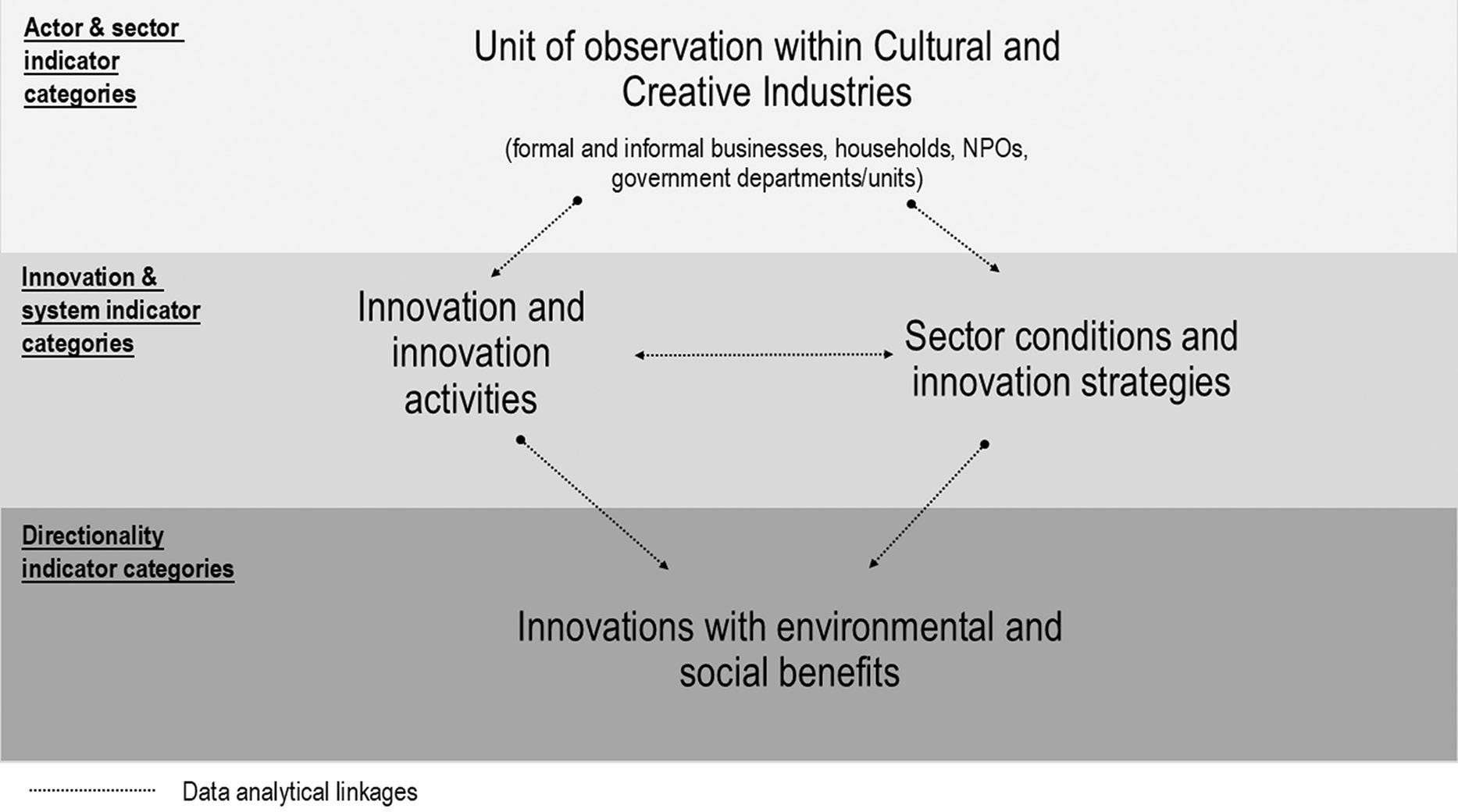
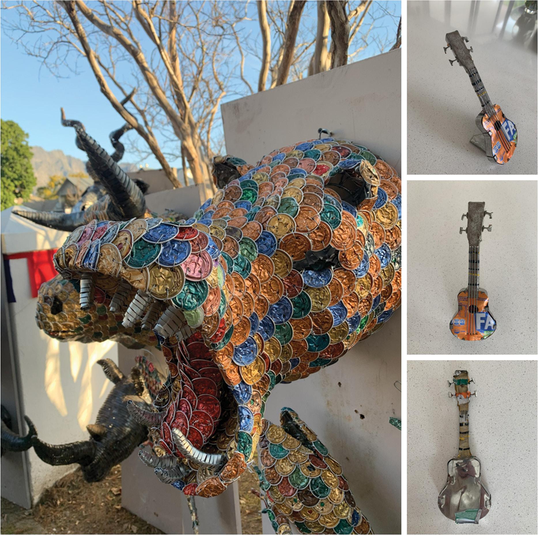
An innovation measurement framework for the South African cultural and creative industries
Gerard Ralphs 61
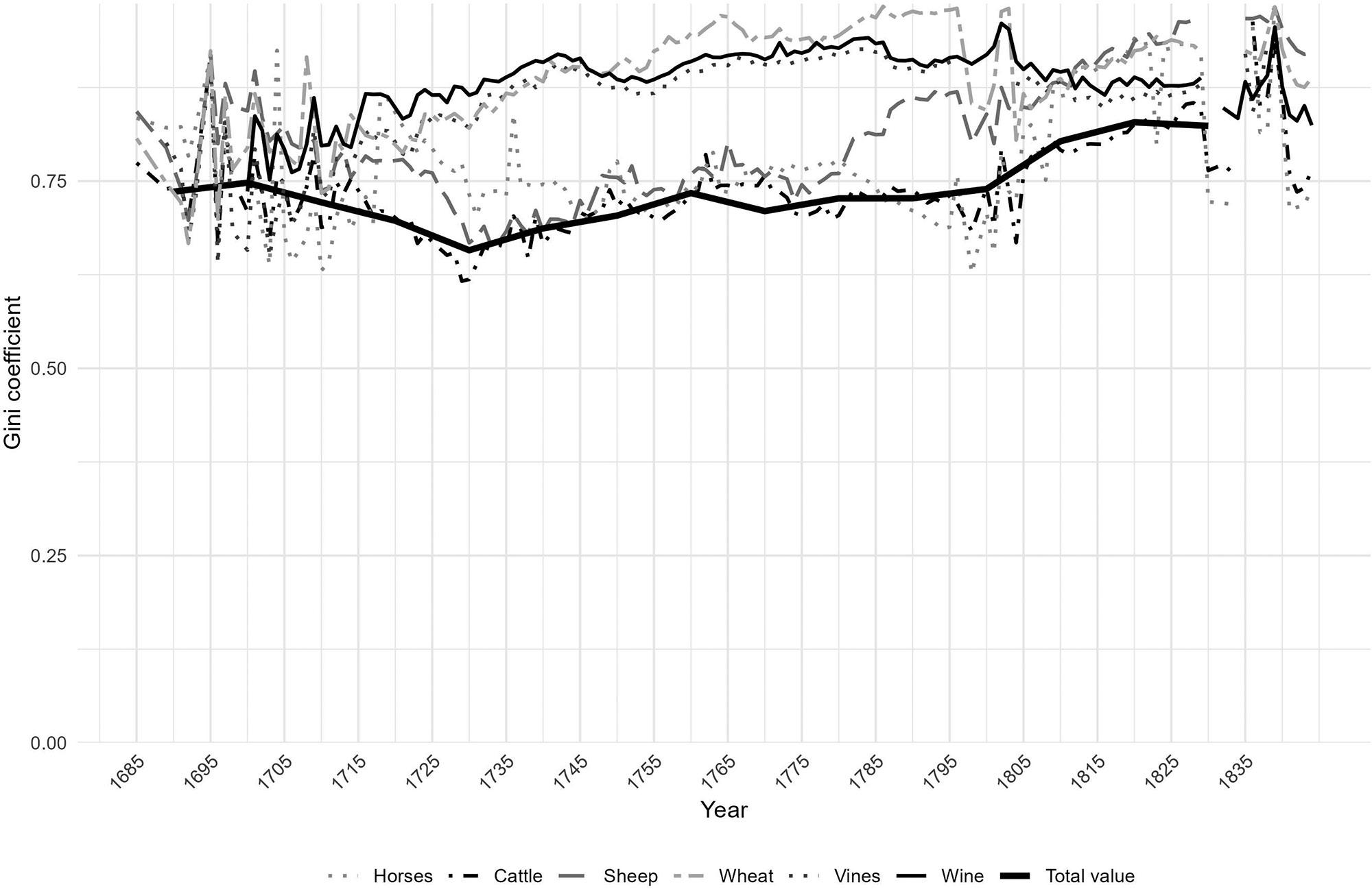
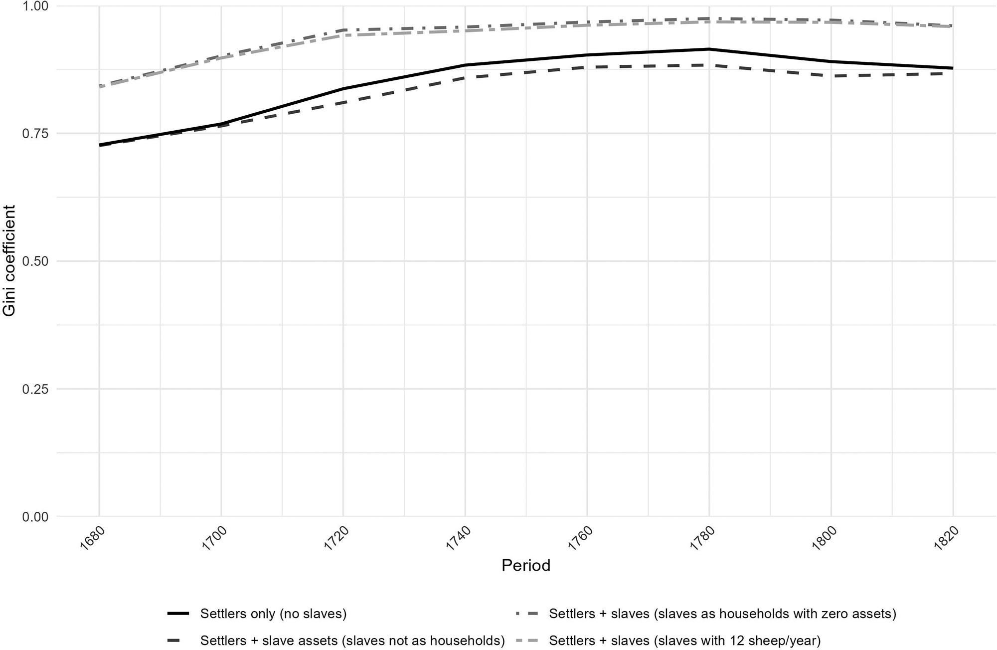
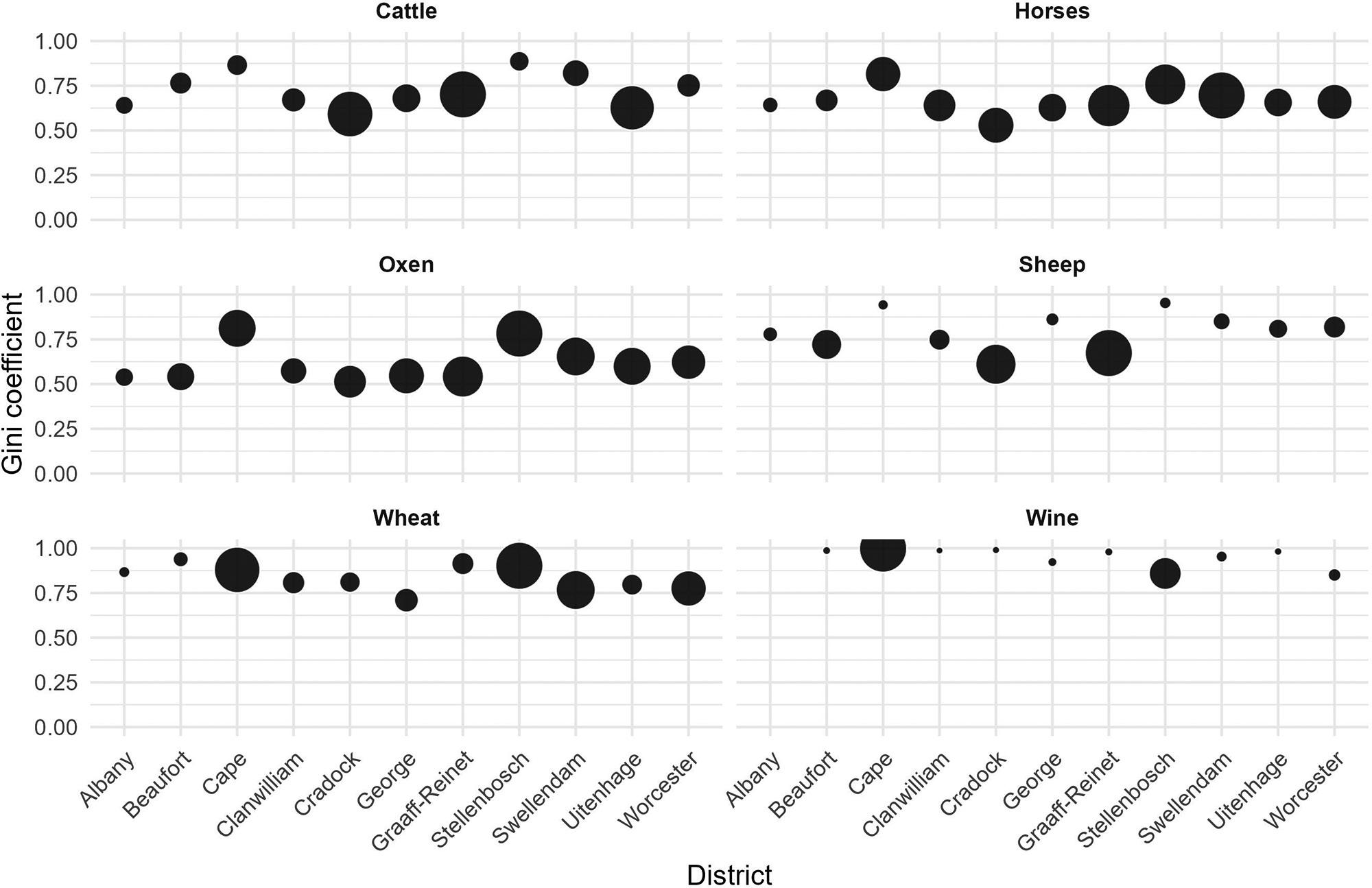
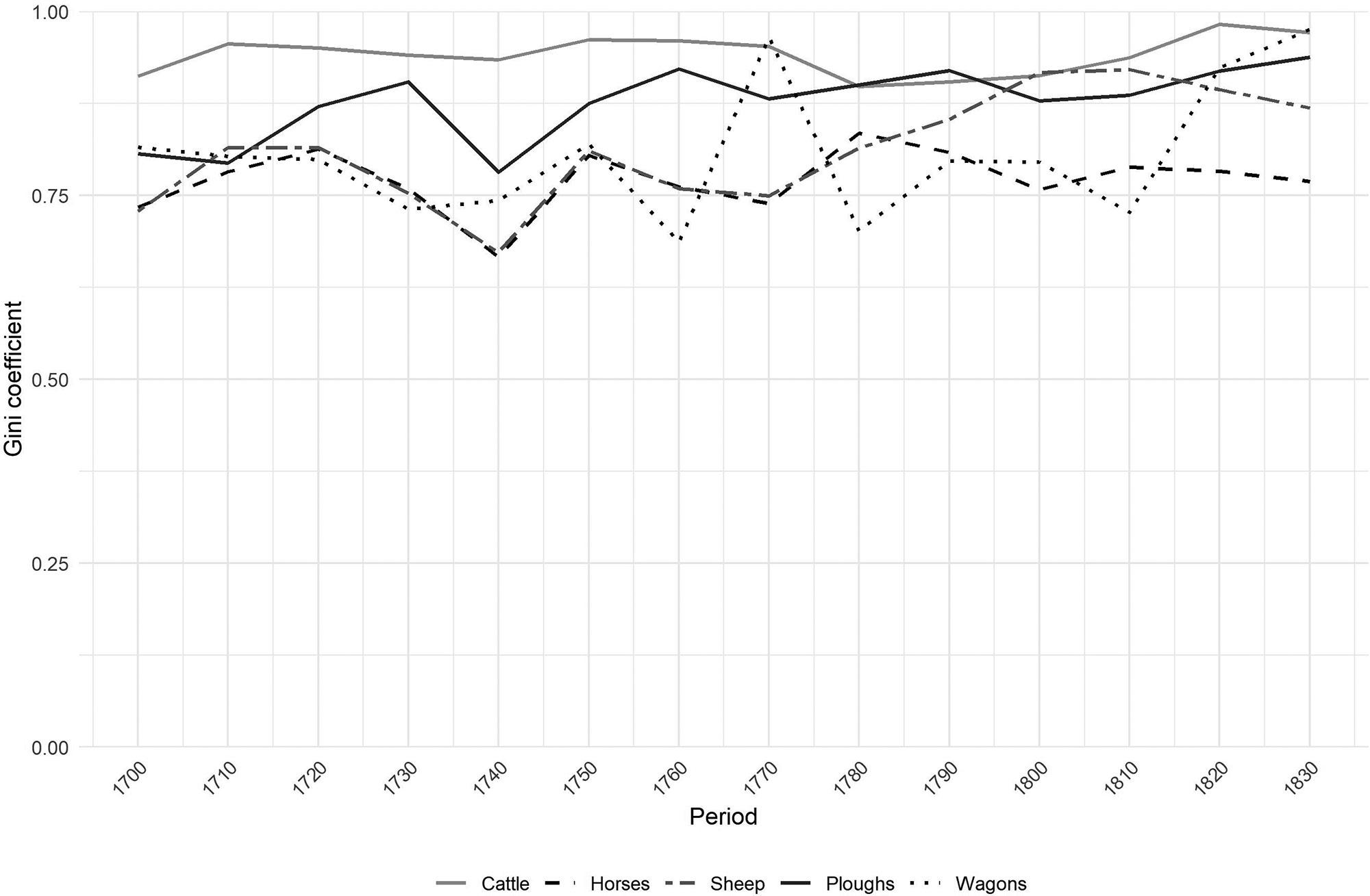
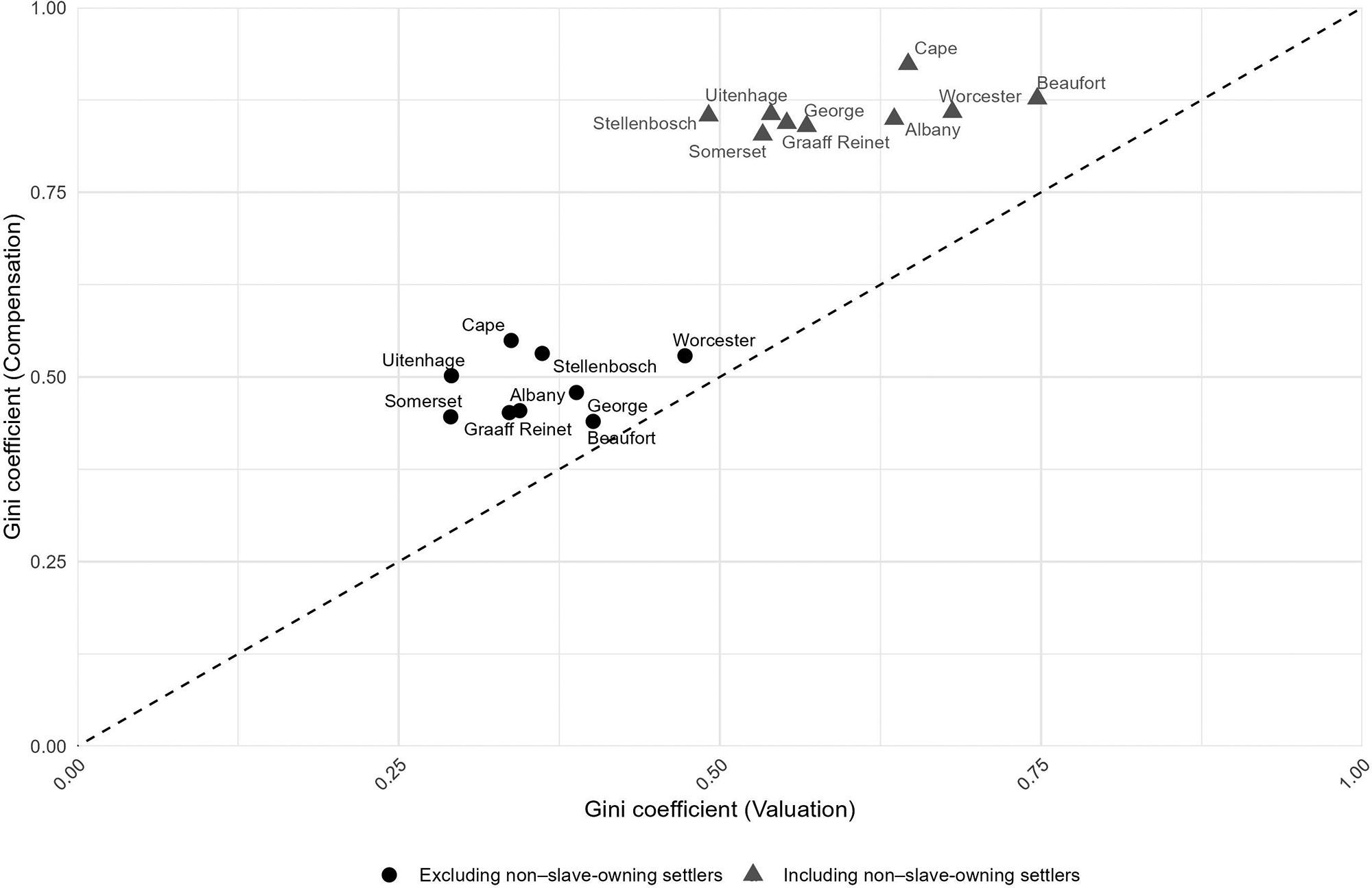
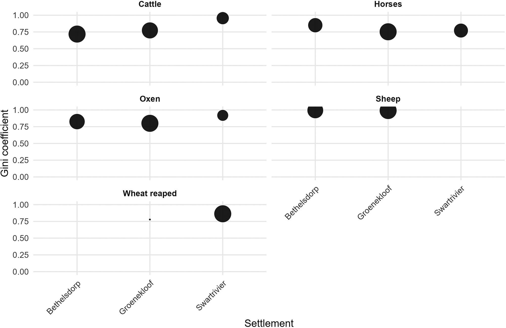
Inequality in the Cape Colony, 1685–1844
Johan Fourie 71
The distribution and status of rooibos (Aspalathus linearis) and its ecotypes in the wild
Tineke Kraaij, Vernon Visser, Gerhard C.P. Pretorius 80
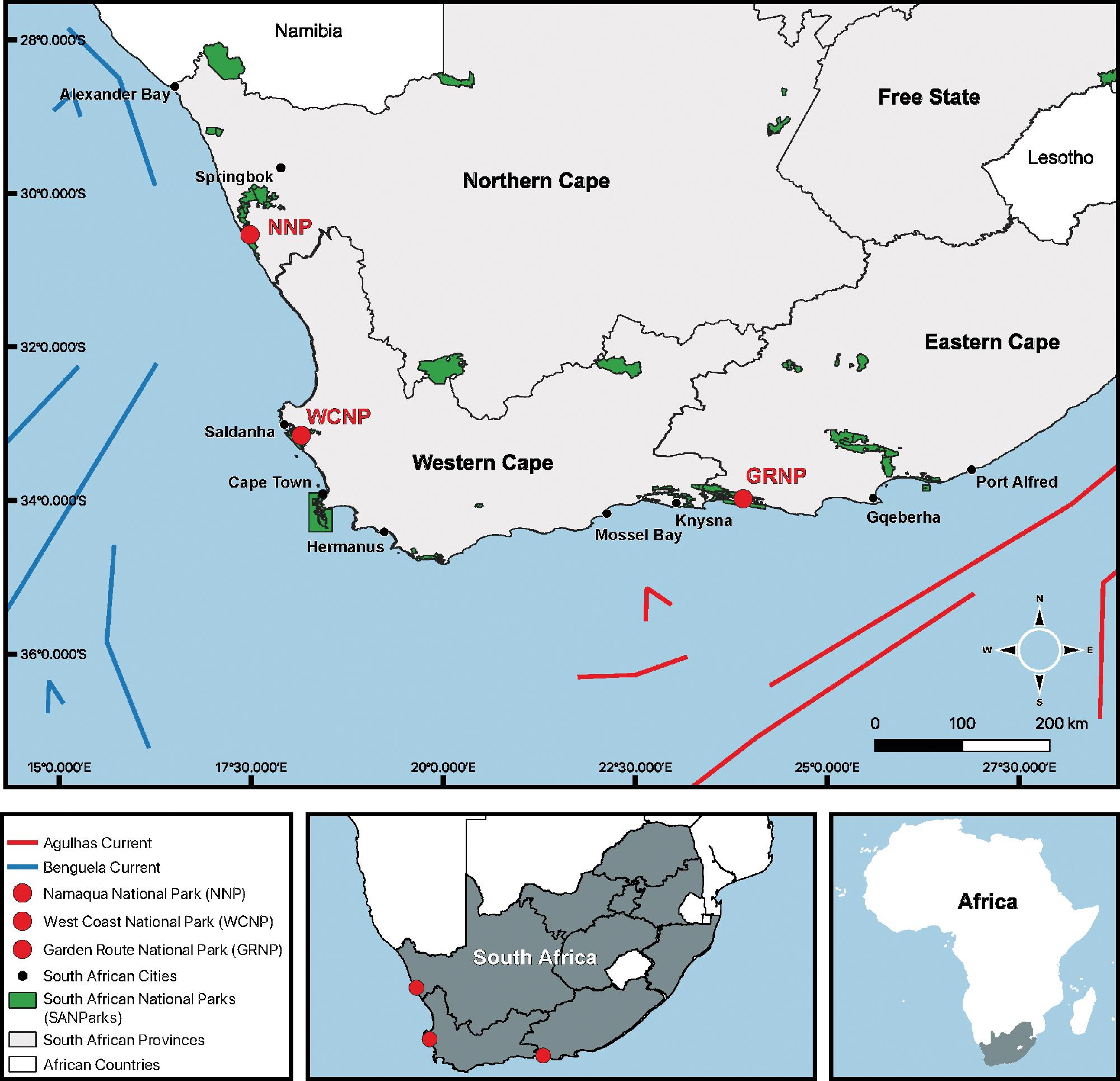
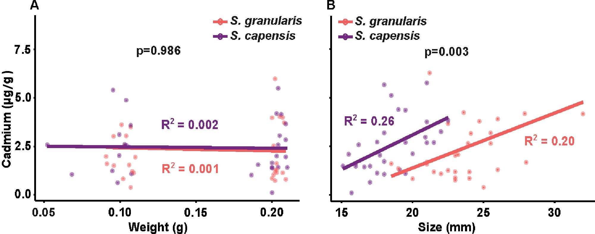
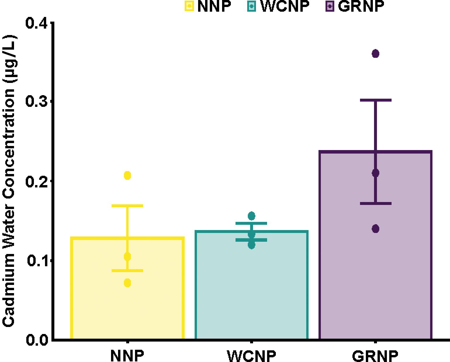
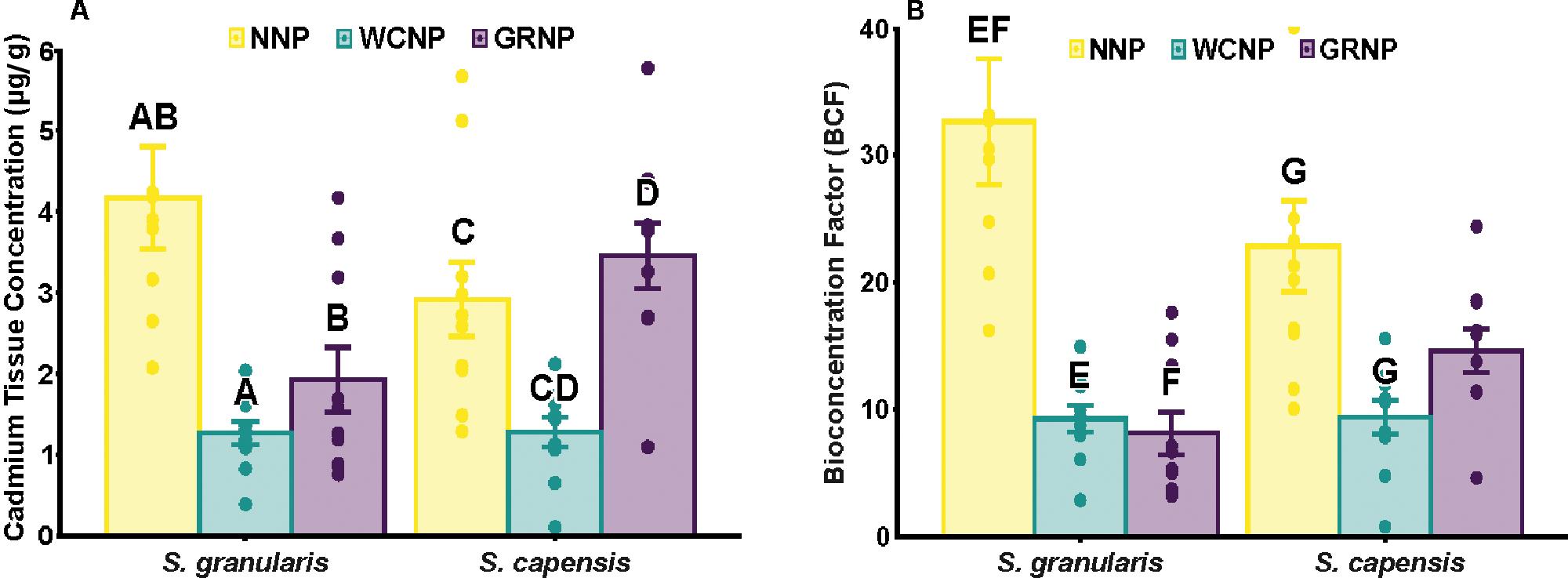
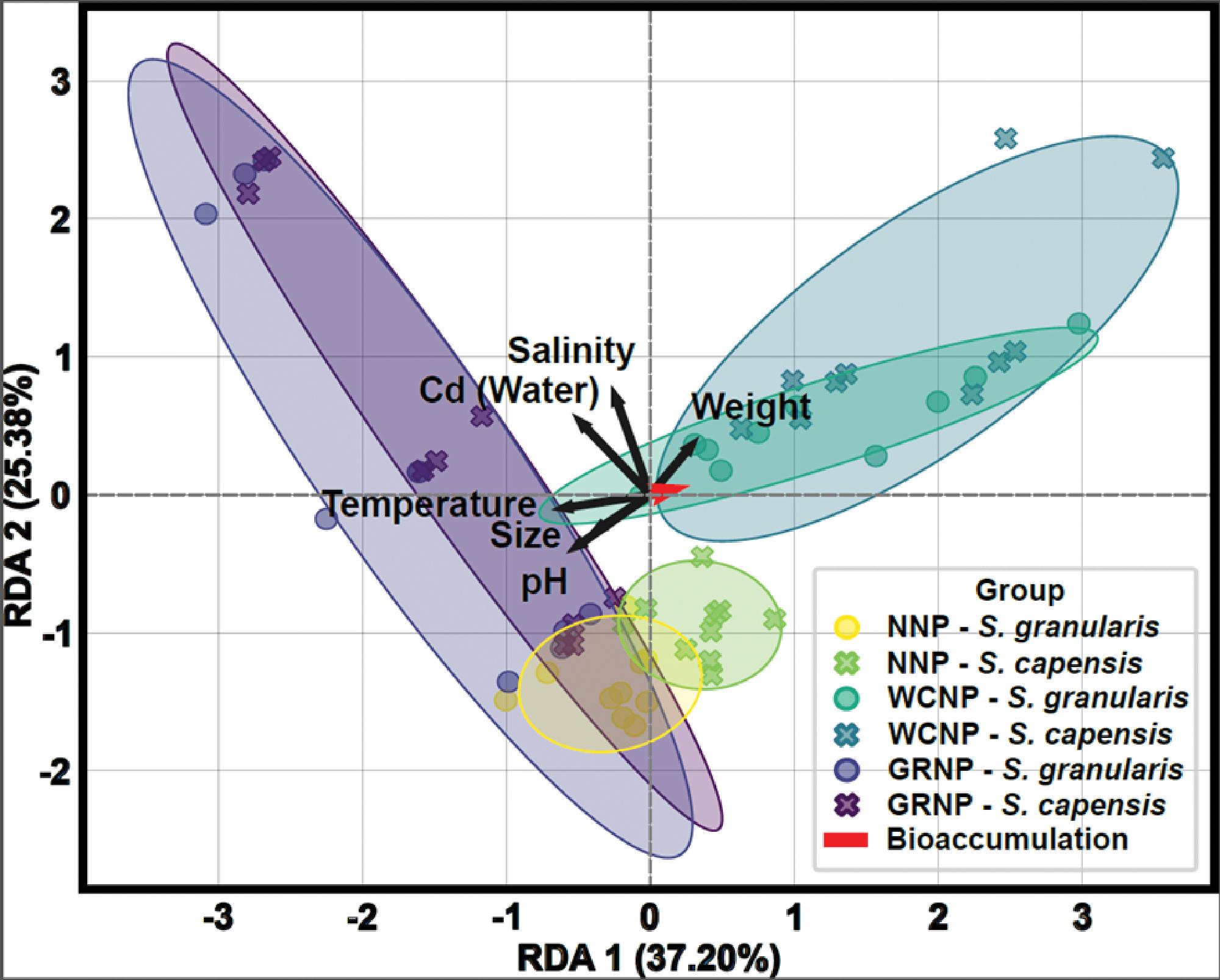
Cadmium bioaccumulation in two resident limpet species, Scutellastra granularis and Siphonaria capensis, along the South African coastline
Liam J. Connell, Kaylee Beine, Richard Greenfield
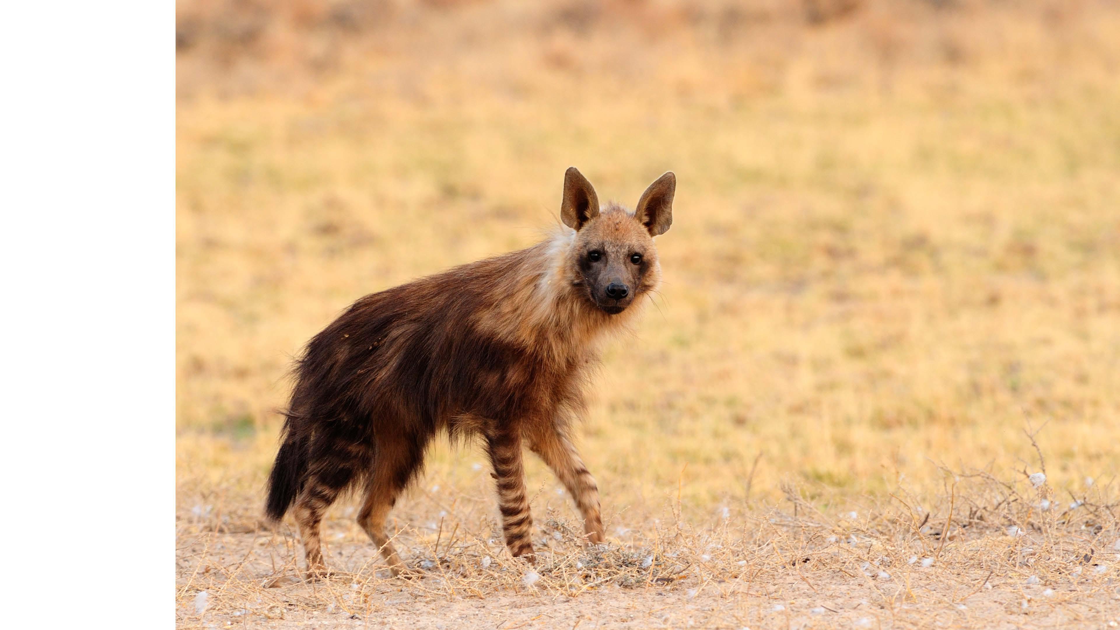
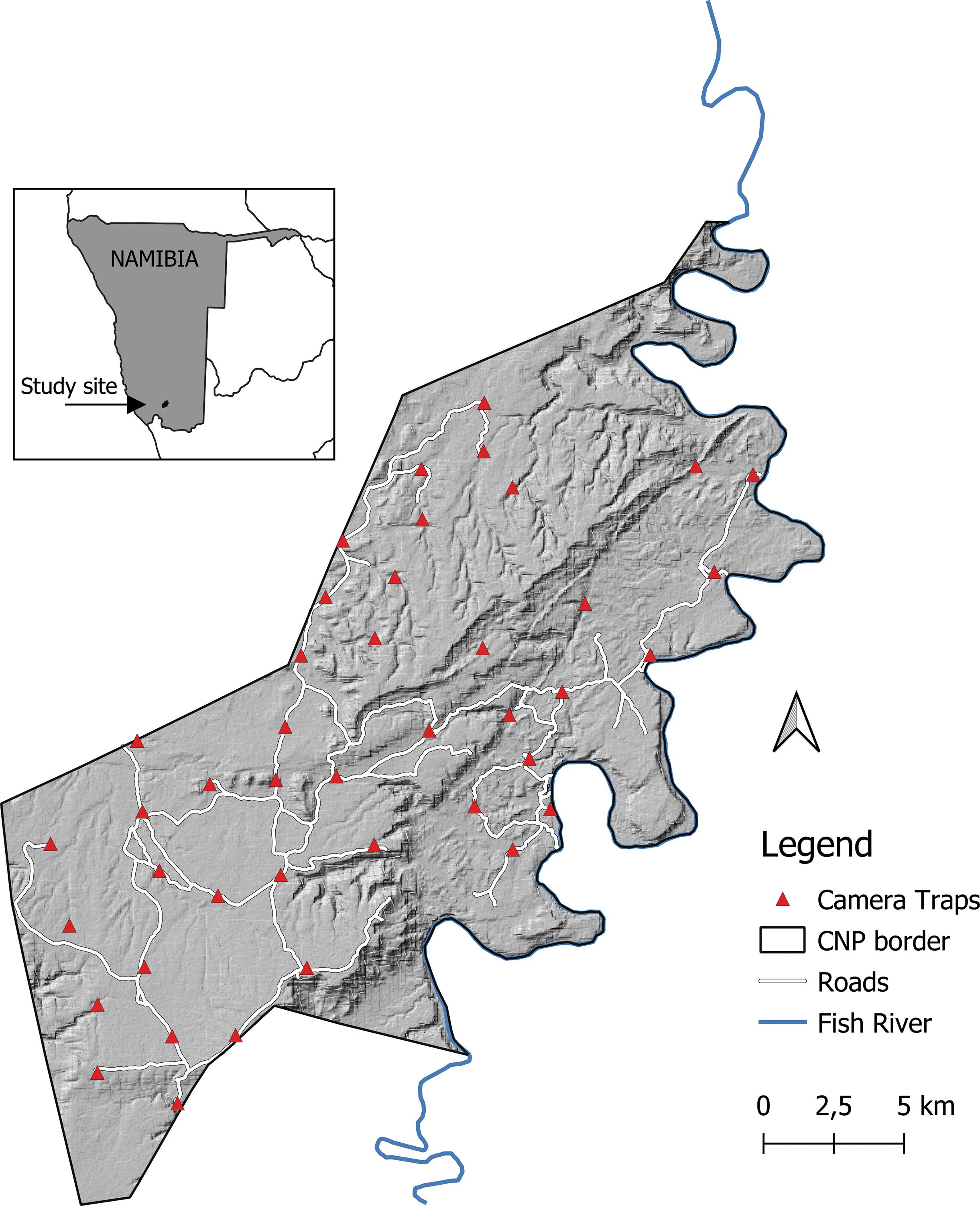
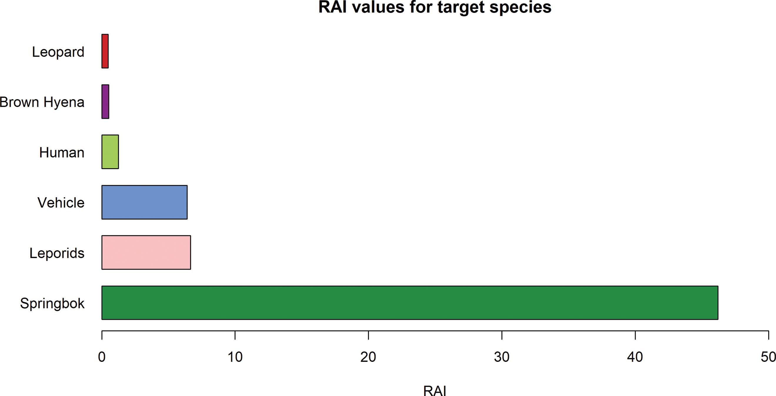
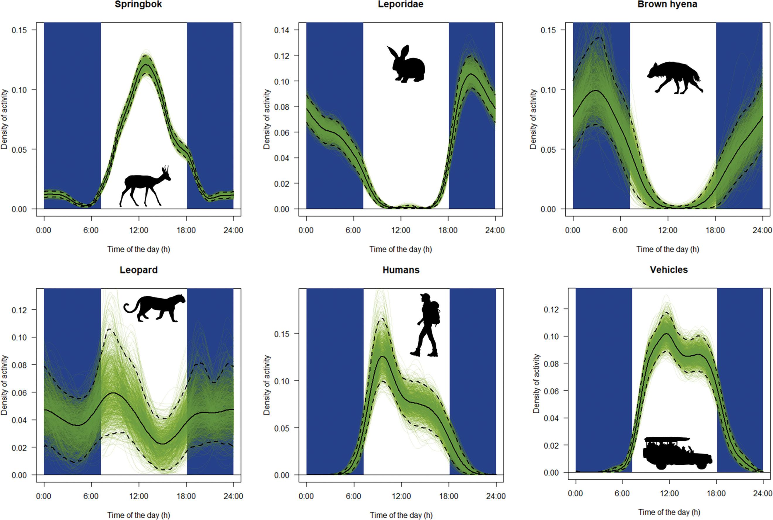
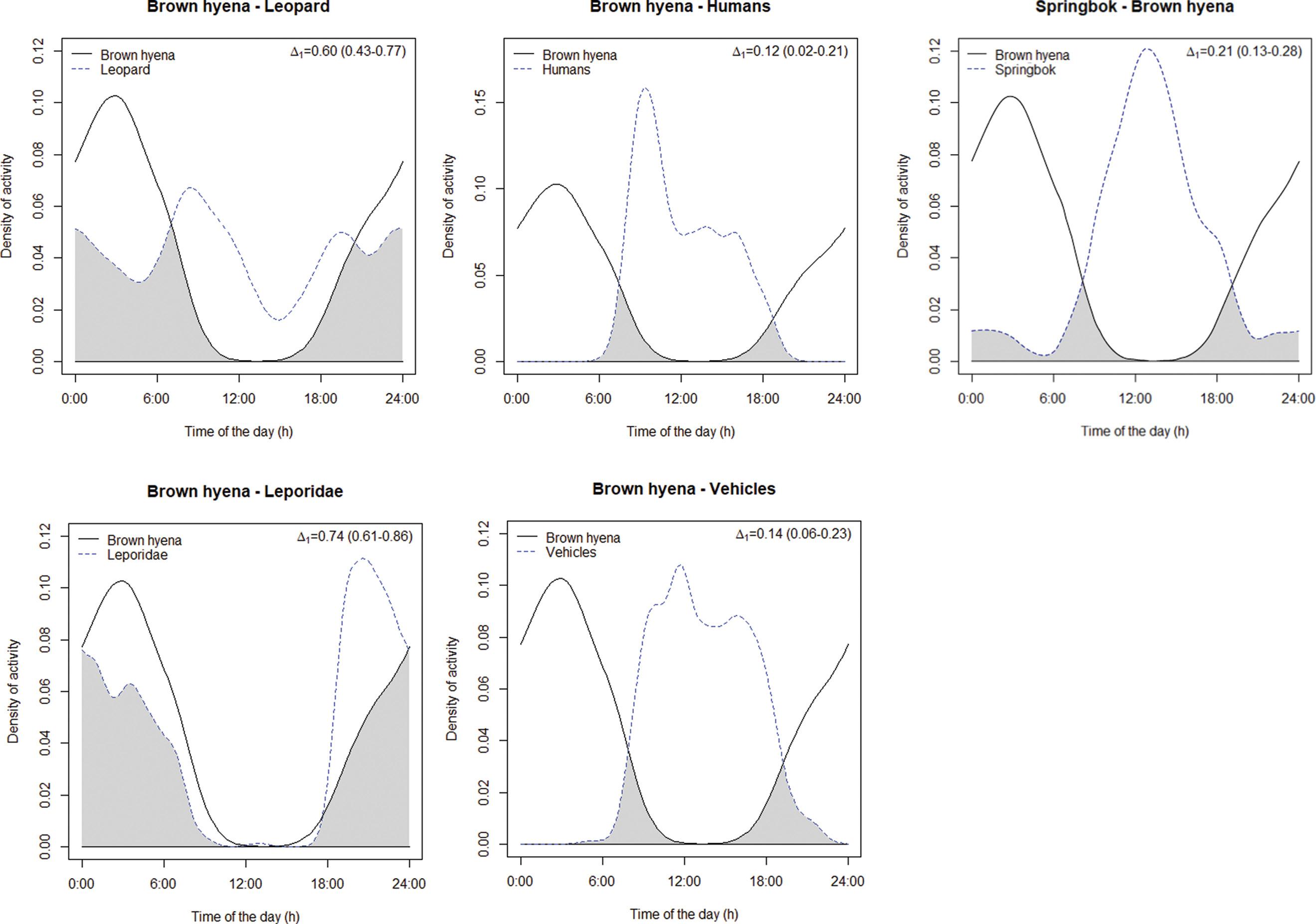
Spatio-temporal behaviour of the brown hyena (Parahyaena brunnea) in the Fish River Canyon, Namibia
88
Veronica Ramello, Ibra E. Monti, Davide Sogliani, Len le Roux, Valentina Isaja, Uakendisa Muzuma, Donato A. Grasso, Maila Cicero, Marta Bormioli, Marcello Franchini, Claudio Augugliaro 95
Research Letter
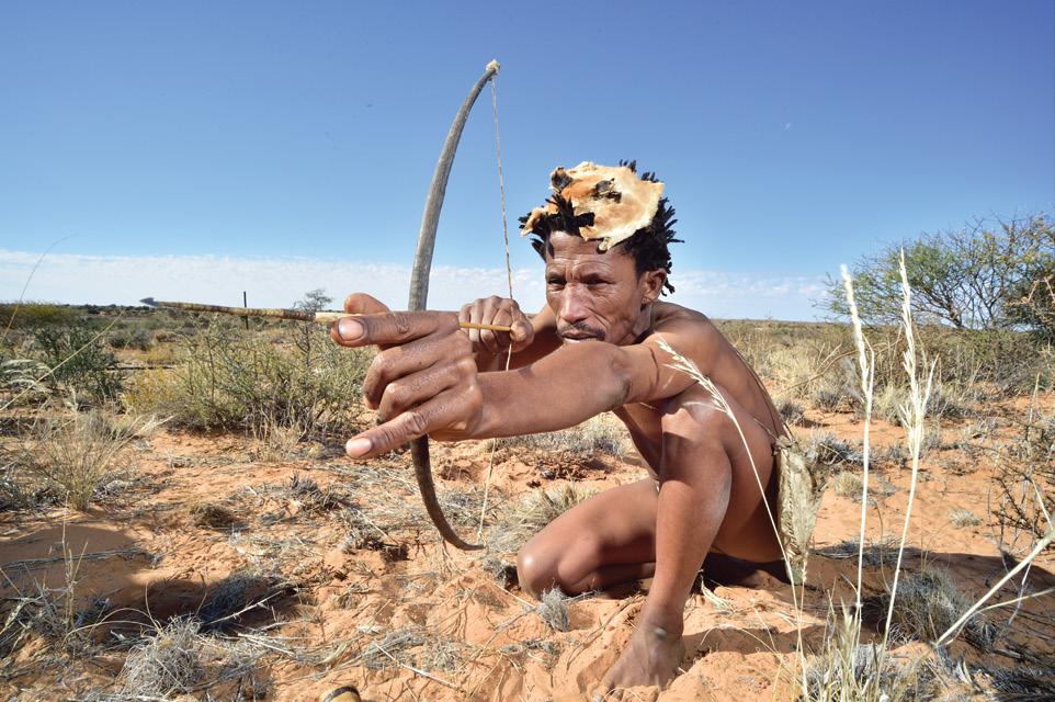
Pleistocene bow-hunting in Africa and the human mind
Marlize Lombard 105
A brown hyena (Parahyaena brunnea). Brown hyenas are found in Angola, Botswana, Namibia, South Africa and Zimbabwe, with almost one-third of the global population occurring in Namibia. Ramello and colleagues describe the spatio-temporal behaviour of the brown hyena in the Fish River Canyon, Namibia.
Climate change, well-being and the rigour of engagement
This year has been an important one for South Africa’s leadership in science. Our country hosted the S20 meeting, centred on the theme of ‘Climate Change and Well-being’. Many South African scientists and science administrators worked very hard indeed to make this important meeting successful, productive and inclusive. All South African scientists, and all South Africans, owe those involved our gratitude. The final statement resulting from the S20 meetings was endorsed by all members.
The Academy of Science of South Africa (ASSAf) was central in the S20 meetings, and hosted the secretariat for the meeting. Our own journal, which is the key journal published by ASSAf, holds a particular responsibility to take the lessons of S20 into the future, and to serve as a forum for publication (subject, of course, to our regular editorial policies and processes) on the S20 theme. Our core identity as an African, multidisciplinary and open-access publication makes us uniquely positioned to advance contextual work on climate change and well-being. As some of our recent special issues show (see, for example, Sustainability Science Engagement and Engaged Sustainability Science, Sustainable Food Systems and How to do social distancing in a shack: COVID-19 in the South African context), along with many stand-alone contributions, applying the best science contextually, and with the benefit of multiple perspectives and approaches, seems key to dealing with difficult and complex societal problems and issues.
ASSAf plays a key role, through its many outreach and other activities, in bringing science to society and society to science, and increasing and diversifying the voices heard in debates about what science is and should be in our context. There can be no question that an ‘ivory tower’ approach to science and knowledge, where expertise rests just with a small group, does not make for the best applied science – multiple voices are needed. In a country with a not very distant history of systematic and legislated segregation and exclusion on the basis of race, gender, class and disability, to name just a few points of exclusion, the need to broaden participation is all the more obvious and urgent. This poses both opportunities and challenges for a journal like ours.
The opportunities are manifold, and as a journal we have over the past few years encouraged wide-ranging and multidisciplinary debates on a range of pressing social issues, as witnessed, for example, by our Discussion Series, explicitly designed to host a range of viewpoints on contemporary topics. We have also expanded our support for new and emerging authors and peer reviewers1, with resources on these topics available gratis through our YouTube channel, to name some of our interventions.
But the challenges are equally important. In a global political context in which right-wing populism has become associated with anti-science views, including views on climate change and on vaccination, for example2, those of us involved in science, science communication and science participation, need to be equally aware of the complexity of the task of embedding science-based evidence in broader social campaigns. Without an informed understanding of questions around politics and participation, science engagement, so key to the S20 theme of ‘Climate Change and Well-being’, can also go very wrong.
Scientists throughout the world are aware at this time that right-wing authoritarian regimes can, and do, create social environments in which there is an erosion of a common understanding of what is the truth, and what the procedural and evidentiary bases are for agreeing that something
HOW TO CITE:
is a fact or not a fact. But it is imperative, in the context of complex multilayered problems, to recognise that there is also value in hearing and trying to understand different perspectives on these problems. Unintended pitfalls can include, for example, co-option of community-based and other organisations in the service of bolstering our credibility as scientists serious about social issues. Especially in a society as unequal as ours, and where poverty is rife, relatively small incentives for community organisations to work with scientists may implicitly encourage these organisations to comply with agendas they did not set and do not want. Finding a compliant voice from what is loosely termed ‘the community’ is not respectful of the complexities and contestations of multiple voices in communities. We need to think about who is saying what, to whom, in what context and why. There are also issues of staging and performativity in community engagement. Sometimes scientists and community activists, whether consciously or not, may play to a co-constructed script of initial hostility and contention, with heated argument, followed by a rapprochement aligned with the views and interests of those who, not uncommonly, have the funding and other resources to stage these events – the scientists. Even more complicated and challenging is the question of who speaks for whom and on what basis various actors claim legitimacy, not only for themselves as players but also as representatives of (sometimes notional and constructed) larger groups. It is a truism of community-based research and the working even of Community Advisory Boards, however important and necessary these may be in community-based science, that these boards, by their very nature, may represent people who are not typical of communities. This atypicality may be present at the outset of a study, by virtue of board members possibly being more articulate, engaged and empowered than others to begin with. Board members may also become less and less representative of communities, less and less like those they supposedly stand for, as they become more absorbed in the scientific process.3
The issues we mention above are just examples of the challenges. Part of our responsibility as a multidisciplinary journal is to be as rigorous in our interrogation of what are often the best-intentioned participatory and community-engaged endeavours, as we are about the best-intentioned ‘hard’ science. For this, we need the benefits of multiple disciplines. Research using inferential statistics is built on the best of scientific scepticism – we need to know that our findings are unlikely to be due to chance. Similarly, rigorous social science approaches will not take at face value declarations that work presents or uses ‘the voice’ of communities or marginalised groups. Good social science interrogates, explores, considers alternative explanations, and questions even what the researchers themselves hold to be true. For good work to be done on questions of climate change and well-being, we need rigorous and transparent methods in all domains. We invite and continue to welcome submissions which show this rigour.
References
1. Finch JM. Academic publishing 101: The SAJS monthly journal writing and peer review forum. S Afr J Sci. 2023;119(11/12), Art. #15753. https://doi.o rg/10.17159/sajs.2023/15753
2. Conway-Moore K, Birch JM, McKinlay AR, Graham F, Oliver E, Bambra C, et al. How populist-aligned views affect receipt of non-COVID-19-related public health interventions: A systematic review of quantitative studies. BMC Public Health. 2025;25(1), Art. #2075. https://doi.org/10.1186/s12889-025-23265-3
3. Carlon C. Contesting community development: Grounding definitions in practice contexts. Dev Pract. 2021;31(3):323–333. https://doi.org/10.1080/ 09614524.2020.1837078
Swartz L, Pietersen D. Climate change, well-being and the rigour of engagement. S Afr J Sci. 2025;121(11/12), Art. #24331. https://doi.org/10.17159/sajs.20 25/24331
AuTHOR: G. Friedrich B. Slabbert1
AFFILIATION:
1President: South African Institution of Civil Engineering (SAICE), Johannesburg, South Africa
CORRESPONDENCE TO: Friedrich Slabbert
EMAIL: president@saice.org.za
HOW TO CITE:
Slabbert GFB. Robert ‘Bob’ Alexander Pullen (1939–2025): A legacy of institutional leadership, technical excellence and dedicated service. S Afr J Sci. 2025;121(11/12), Art. #23544. https://doi.org/10.17159/sa js.2025/23544
ARTICLE INCLuDES:
☐ Peer review
☐ Supplementary material
PubLISHED: 26 November 2025
Robert ‘Bob’ Alexander Pullen (1939–2025):
A legacy of institutional leadership, technical excellence and dedicated service
On 27 May 2025, South Africa’s engineering fraternity lost one of its most influential and steadfast pillars — Robert ‘Bob’ Alexander Pullen. His passing leaves a legacy of institutional leadership, technical excellence and dedicated service to the built environment and the communities it supports.
Bob Pullen was born on 2 December 1939 in Benoni and spent his formative years in Rustenburg, where he matriculated in 1957. He went on to graduate from the University of the Witwatersrand (Wits) in 1963 – a milestone that would mark the beginning of a lifelong journey of scholarship, practice and service. He completed his MSc(Eng) degree under Prof. DC Midgley. In 1964, he took a position as research engineer in the Hydrological Research Unit at Wits. In 1969, he joined the Department of Water Affairs in the Planning Division. He joined Steffen Robertson & Kisten in 1982. Over the years, he would come to be recognised not only as a brilliant civil engineer, but as a statesman of the profession, bridging technical, regulatory and institutional needs with vision and integrity.
Professional journey and contributions
From the early stages of his career, Bob positioned himself in roles that spanned technical engineering, policy, regulation and professional governance. As a consulting engineer, his expertise lay primarily in water resource evaluation and development, hydraulic engineering, and environmental and institutional management – disciplines that demand not only technical skill but the capacity to see systems, impacts and long-term sustainability intimately entwined.
One of his signature contributions was his involvement in the editorial and technical work behind the 1986 Department of Water Affairs document ‘Management of the Water Resources of the RSA’, colloquially regarded as South Africa’s ‘water bible’. In that role, he helped shape national policy frameworks on water management that would endure for decades. He also played a central part in investigations of major floods, the development of national flood management policy, and in legislating disaster and environmental planning in South Africa.
This technical foundation and his reputation for fairness and consensus-building naturally led to roles of governance and professional regulation. He served on the Council of the South African Institution of Civil Engineering (SAICE) from 1972 until 1997, and in 1989 he was elected President of SAICE.
However, his most enduring institutional impact may have been at the Engineering Council of South Africa (ECSA). Elected unanimously, Bob served three terms as President from 1994 to 2006 and continued as Vice-President until 2008. Under his guidance, ECSA navigated a period of transition in South Africa’s constitutional order, culminating in the promulgation of the seven Built Environment Professions Acts in 2001 – legislation that harmonised the regulatory framework for engineering and allied professions in the new democracy.
In recognition of his service, Bob was named an Honorary Fellow of SAICE and was awarded a Gold Medal by Wits University (through its alumni/honorary degree citations).
In 2009, Bob was honoured with the National Science and Technology Forum (NSTF) Award (Category C) for his contributions outside pure research, in policy, regulation and professional practice – underscoring his impact beyond academia into the broader science, engineering and innovation community.
His influence extended beyond national boundaries. He served as past President of the South African Academy of Engineering (SAAE), and was, for many years, Chair and champion of ECSA’s role in transforming South African professional regulation.
Leadership, philosophy and legacy
Bob Pullen’s professional ethos balanced technical depth with institutional wisdom and a strong moral compass. The late Dawie Botha, SAICE’s Executive Director, said in 2014, that Bob warned against the commodification of professionals – the risk that engineers might be judged by the bottom line rather than the excellence and integrity of their service.
His knack for diplomacy, fairness and consensus – traits often praised by his peers – allowed him to navigate contested policy landscapes and bring multiple stakeholders into alignment.
Bob was also ahead of his time in embracing the overlap between the environment and engineering. Even before ‘sustainability’ became a buzzword, he promoted the idea that environmental systems must be integrated into engineering decisions and that the built environment must co-exist responsibly with nature.
His service extended to mentorship, institutional capacity-building and nurturing the next generations of engineers. Whether in SAICE’s institutional programmes, ECSA’s regulatory evolution, or academia’s links to practice, Bob was a bridge-builder. He served as a member of the SAICE Council from 1972 to 1997, was elected Honorary Fellow in 1996, and awarded SAICE’s prestigious Gold Medal in 2001.
His retirement from active governance did not diminish his influence; his counsel remained sought and respected.
Bob Pullen’s contributions to the Academy of Engineering were both substantial and sustained.
• He was elected as a Fellow of the SAAE – Independent Civil Engineering Consultant: Water Resources Development, Environmental Impact Management, Programme and Project Management, Mentoring of Young Professionals.
• He served as President of the SAAE for a two-year term covering 2014–2015. Under his Presidency and leadership, the Academy aligned itself with its mission to mobilise the collective wisdom of eminent engineers in South Africa “in the interest of the public, not in the interest of its members.”
• Bob also continued his involvement after his term as President. For example, in later years, he served on the Executive Committee in the capacity of Past President/Treasurer.
• Beyond national work, as part of the SAAE, he participated in international engineering academy networks; for example, Bob represented the SAAE at the Council of Academies of Engineering and Technological Sciences (CAETS) Convocations.
Bob’s SAAE role was a senior institutional leadership one – beyond being a member or contributor, he stepped into presidency and governance, helped position the Academy within national and global engineering discourse, and thereby helped shape an institution aimed at engineering and policy advice in South Africa.
Personal and community life
Behind the titles and achievements was a man of quiet determination, humility and integrity. He was known to be supportive, approachable and generous with his time, especially to younger engineers seeking guidance.
In 1965, Bob married Dee Lawrence in Johannesburg; they had five children: three daughters and twin boys. Bob and Dee lived a full life in their community and affairs of their society. Bob was the golf captain of the Pretoria Country Club for a few years and served on the Club Management Committee.
In his later professional years, he served as Senior Specialist in Water Engineering at BKS (Pty) Ltd, contributing to policy, project oversight and mentorship within the firm.
He is survived by his family and the countless professional colleagues and mentees who carry forward his values of service, excellence and ethical stewardship of infrastructure and institutions.
A final reflection
In 1989, as SAICE President, Bob represented a leadership grounded in technical credibility, institutional engagement and a deep appreciation for the public good. Over the ensuing decades, he translated that ethos into architecting the regulatory and institutional scaffolding that would help South Africa’s engineering profession adapt, endure and serve more inclusively. He walked in the delicate intersection between engineers, regulators, academia and government, often quietly, often without fanfare – yet always with principle and impact.
His passing invites us to reflect on the attributes that sustain a profession through turbulent times: courage to speak truth to power, generosity to mentor, patience to build consensus, and fidelity to service over self. In honouring his life, the engineering community must also recommit to those ideals.
May his family and loved ones find comfort in shared memories and may the South African civil engineering community – SAICE, ECSA, academia, and beyond – continue to reflect on Bob’s legacy and carry forward the responsibility he so faithfully bore.
https://doi.org/10.17159/sajs.2025/23544
Bob Pullen at the Inauguration of the 122nd President of the South African Institution of Civil Engineering (SAICE) in 2025 (image: SAICE).
bOOK TITLE: On Discovery: How Knowledge is Produced across the Disciplines
EDITOR: Jonathan
Jansen
ISbN: 9781009596596 (paperback, 325 pp; USD36)
PubLISHER: Cambridge University Press, Cambridge
PubLISHED: 2025
REVIEWER: Wieland Gevers1
AFFILIATION:
1Emeritus Professor of Medical Biochemistry, University of Cape Town, Cape Town, South Africa
EMAIL: wieland.gevers@uct.ac.za
HOW TO CITE: Gevers W. Comparing like and unlike: Discovery through knowledgeable commitment in every discipline. S Afr J Sci. 2025;121(11/12), Art. #23771. https://doi.org/10. 17159/sajs.2025/23771
ARTICLE INCLuDES:
☐ Peer review
☐ Supplementary material
PubLISHED: 26 November 2025
Comparing like and unlike: Discovery through knowledgeable commitment in every discipline
2025. The Author(s). Published under a Creative Commons Attribution Licence.
I greatly enjoyed reading all the chapters of this book, and suspect that many other readers will do the same. Jansen has chosen as a representative sample a relatively self-contained group of South African researchers who could be said to be internationally somewhat ‘marginalised’ or ‘provincial’ but are remarkably competitive all the same. They are also settled in the complex context of their home country, making it possible to draw some additional conclusions about positionality in knowledge discovery. Each of the 22 authors has been asked to write their account in the first person, bringing focused subjectivity to bear on the intended objectivity of the topic of how new knowledge is generated in a large number of sometimes sharply contrasting disciplines.
Traditional scholarly disciplines have in recent times become conceptual and methodological silos as their individual knowledge domains have vastly expanded and even fragmented internally to create sub-silos; the minds of their practitioners appear to have become so ‘structured’ that perspectives are shuttered and restricted to one way of looking at the world. Advocates of ‘consilience’ (all disciplines are dealing with but one reality1) and of multi-, trans- and cross-disciplinarity, as well as ‘Mode 2 research’, have an uphill battle against the entropic forces that drive specialisation. Readers of this book (and I hope there will be many) emerging from their own thought-worlds will at times be impressed, amazed, puzzled or horrified as they encounter the pre-occupations of their fellow researchers in other disciplines. As they all have in common a basic degree of common sense and intelligence, they may consider the questions to which answers are sought as intriguing, ill-conceived, trivial or even pointless. Alternatively, they may believe that they are able to devise a different way to reach the answer to a question being addressed in a particular way in a different discipline. As just an example, they may be unhappy when a distinguished moral philosopher (Thaddeus Metz) seeks to determine “the meaning of (human) life” when over 8 billion people on earth each have their own unascertained view on the matter and the words ‘meaning’ and ‘life’ are undefined to anyone’s satisfaction in any case. Yet the scholar in question, through further reading and reflection, has been able to use the topic as a starting point for addressing, in a unique manner, important moral issues in multicultural human societies.
Some of the chapters (for example those of the surgeon Elmi Muller and the astronomer Justin Jonas) illustrate how technical breakthroughs (some ‘in the hands’ and some in high technology) are also ‘new knowledge’. Scrutiny of lists of Nobel Prizes will bear this out as well: a new technique can open the floodgates of the elaboration of expanded knowledge about natural processes or diseases. A good example might be drawn from Jansen’s citation of Frederic Holmes’s brilliant description of Sir Hans Krebs’s discovery of his eponymous metabolic cycle in the 1930s.2 Major advances in techniques have confirmed the cycle’s basic features but have permitted a massive elaboration of its workings in living cells in different situations and organisms, not the least being that the cycle often goes in the reverse direction when the emphasis is on growth and not on energy generation.3
Jansen’s concluding chapter is a masterly synthesis, drawing on all 22 chapters (including his own) to sort the main issues under appropriate headings, some of them ingenious neologisms. These sometimes overlap but are helpful ways of putting together the bigger picture of how new knowledge is sought and found in different disciplines. They are, respectively, the “classical model of scientific discovery” (but see below), differentiability, positionality, serendipity, non-linearity, indeterminacy, technicity, foundationality and pragmatism. This analysis seems to be the last word on the book topic, but two quibbles may be worth mentioning. Firstly, one essential heading is missing – disruptiveness – where one person or group doggedly bucks prevailing ideas to establish a new paradigmatic notion that will enable previously unsolved issues to be addressed (one author – Thulani Makhalanyane – discusses this issue briefly in his chapter.) Secondly, Jansen’s use of a clinical trial to exemplify the “classical model of scientific discovery” is not fully appropriate as it covers only those domains of discovery that deal with populations of similar but variably differing organisms. Much “classical” research, by contrast, deals with finding out how a particular process in nature works or, in the applied version, can be made to work reproducibly and efficiently to meet needs of many kinds. These discoveries are not so easily falsified by subsequent work in the Popperian or Kuhnian senses, but readily extended and elaborated upon to build a reliable edifice of knowledge.
It is noteworthy that Jansen, the immediate past president of the Academy of Science of South Africa, has overseen the conceptualisation and realisation of this book, with its remarkable assembly of contrasting chapters offering a genuine insight into the practice of science (in the broad sense of the word) in South Africa at the present time. This follows on the Academy’s production of The State of Science in South Africa in 2009, which includes comprehensive descriptions of the principal pre-occupations in the country in each of the major disciplines4, and the publication of Legends of South African Science in 2017, which provides vignettes of scholars who have received certain prestigious awards5. The three books complement each other admirably, each bringing out a different important aspect of the country’s overall knowledge-generating system.
I strongly recommend this very readable and significant book to all who are willing to widen their view, consiliently, to discover the world and its inhabitants and constituents in all their glory and complexity. They will agree with Jansen that the intrinsic value of research, grounded in deep knowledge and reflection and driven by curiosity, is its own reward irrespective of discipline.
References
1. Wilson EO. Consilience: The unity of knowledge. New York: Alfred A Knopf and Co; 1998.
2. Holmes FL. Biochemistry. New Haven, CT: Yale University Press; 2001.
3. Lane N. Transformer: The deep chemistry of life and death. London: The Profile Press; 2022.
4. Academy of Science of South Africa (ASSAf). The state of science in South Africa. Pretoria: ASSAf; 2009. http://hdl.handle.net/20.500.11911/65
5. Academy of Science of South Africa (ASSAf). Legends of South African science. Pretoria: ASSAf; 2017. http://hdl.handle.net/20.500.11911/74
bOOK TITLE: A Widening Idea of Health and Health Research: The South African Medical Research Council from Creation to COVID
AuTHOR:
Howard Phillips
ISbN:
9781067235215 (hardback, 176 pp)
9781067235215 (ebook, 176 pp)
PubLISHER:
South African Medical Research Council, Cape Town
PubLISHED: 2024
REVIEWER: Julie Parle1
AFFILIATION:
1Department of Historical and Heritage Studies, University of Pretoria, Pretoria, South Africa
EMAIL: Julie.parle@up.ac.za
HOW TO CITE:
Parle J. Medical research, evidence and politics: An insightful history of the South African Medical Research Council, 1969–2022. S Afr J Sci. 2025;121(11/12), Art. #22595. https://doi.org/10.17159 /sajs.2025/22595
ARTICLE INCLuDES:
☐ Peer review
☐ Supplementary material
PubLISHED: 26 November 2025
Medical research, evidence and politics: An insightful history of the South African Medical Research Council, 1969–2022
Written by South Africa’s most distinguished medical historian, Emeritus Professor Howard Phillips, this is both a richly illustrated and attractive book (available as a free download) and a well-timed, thought-provoking institutional history. More than this, A Widening Idea is also a subtly insightful analysis of the intertwined fates of the modern South African state (both apartheid and democratic), medical science research, the hard realities of paying for it, and contests over health policy.
Across six chapters, which correspond with different ‘eras’, Phillips takes us from the foundation in 1969 of the South African Medical Research Council (SAMRC) by the apartheid state through to 2022, with the COVID-19 pandemic still not quite over. He charts and assesses the legislative, organisational, financial and research trajectories of the numerous research units, institutions and groups under the aegis of the SAMRC over more than half a century.
The book opens with a reminder that statutory organisations such as the SAMRC are always dependent on the state for financial, administrative and political support. Unsurprisingly, their public documentation is likely to be burnished by a positive spin. Yet, a wider story is a truer and more transparent one, likely more helpful in an organisation’s assessment. Therefore, this book strives to show not only the SAMRC’s many important scientific and medical accomplishments, but also its “missteps”. This was made possible by consulting other sources, from archives and newspapers, and through the nearly 40 people interviewed by Phillips.
In its early years, the SAMRC was mostly compliant with apartheid ideology and goals. Since 1994, at notable times, SAMRC presidents have found it necessary to demonstrate the body’s independence from misguided state interference and, on occasion, its own Board. They did so by drawing on the authority of medical science to “speak truth to power”, crucially since the 1990s in service of a democratic society. Thus, the authority and legitimacy of the SAMRC has widened.
Lest you be concerned that the book is a hard slog of a read, I can reassure you that it has a healthy dose of what I have come to call ‘HP sauce’. It is written in prose that is sometimes sharp (in insight) and is peppered with puns that sometimes occasion a smile (or a wince), especially in the chapter titles and many picture captions, with the overall effect of adding interest and flavour.
Chapters 1 and 2 (1969 to 1985) cover the SAMRC’s origins and structure. Across the globe, World War II demonstrated the value of modern medical research to the state. Phillips states, unequivocally, that in South Africa this was to be in the service of “the creation of a white welfare state… informed by the latest ideas in Western science, medicine and technology” (p.4). An apartheid Parliament provided the bulk of the SAMRC’s funding. Afrikaans-speaking men dominated, English speakers were tolerated, and black South Africans only as “menial workers”. Even the conceptualisation of the research was based in scientific racism; the inhabitants of the country being understood as different peoples, with different illness aetiologies and needs.
Structurally, the SAMRC follows a hybrid model, with the research it funds being carried out by a mixture of ‘in-house’ or intramural institutes or centres and extramural research units, groups, and short-term researchers at a growing number of universities. Those institutions that were reserved for white people benefitted disproportionately in these decades. This has left a complicated legacy.
During the years of high apartheid, to 1985, the SAMRC gained in self-confidence, although its relationship with other bodies, including the Department of Health, was not without friction. Yet, increasingly, the research conducted showed greater complexity than this racially segregated state-imposed grid sought, and researchers at times showed agency, integrity and ambition. For instance, research into oesophageal cancer in the Transkei led to both scientific acclaim and successful preventive measures.
By the mid-1980s, the transition towards democracy was underway at the SAMRC as well as nationally (Chapter 3). Initially with the intention of reforming apartheid, there was a recognition that the “emphasis hitherto on pathological, clinical and laboratory-based research” was too limited to “overcome the country’s health challenges” (p.33); instead, the SAMRC widened its efforts to encompass primary health care.
The South African Medical Research Council Act 58 of 1991 reflected the country’s democratic aspirations, in the service of “the health of the population of the Republic” (p.49). As one health rights medical researcher was soon to note (p.71), however, it was necessary to get “the right combination of science, evidence and politics to succeed”. Getting these in alignment has proved tricky amongst economic restraints, sometimes bumpy politics, and drastic medical crises.
Reconstruction and transformation (Chapter 4) were the watchwords of Malekapuru Makgoba, Chair of the SAMRC Board from 1994 to 1998, and its President, 1998 to 2002. These were to be “grounded in the Constitution, and the best scientific values” (p.53). Phillips describes Makgoba’s terms as characterised by “transformative ardour”. The organisation was expected by the ANC and its alliance partners to set an example for other parastatals. Some transformation initiatives worked better than others.
Makgoba was responsible for driving the expansion of research, both scientific and socio-economic, into the AIDS epidemic, which at that time was escalating on a terrible scale. By the early 21st century, South African
medical science researchers were no longer “contributors” to clinical trials for HIV vaccine trials, but “drivers” (p.59). Unfortunately, a vaccine breakthrough did not come.
Phillips deals judiciously with the clash over AIDS between Makgoba, Mbeki and the latter’s ideologically loyal but scientifically misguided health ministry. Makgoba stuck to his guns and insisted in words that today, a quarter of a century later, have resonance for medical and other scientists across the world: “… it’s not about who’s in charge of this country, it’s about what the evidence is saying” (p.62). In asserting the legitimacy of evidence-based medical research, the medical profession and civil society, notably the Treatment Action Campaign, had found their voice in speaking out for science – a further widening of the importance of the SAMRC. AIDS and TB research became even more central, but so too did other areas of applied research – topics (to name but a few) included women’s health, children, rape, domestic violence, gun crime, and alcohol and drug abuse. Violence, it was recognised, “is a part of our country’s history” (p.67). Along with laboratory-based studies and findings, this long chapter minutely details dozens of innovative and important research projects and groups which, now being published in major journals and impacting policy debates within South Africa, widened the SAMRC’s reach nationally and internationally yet further. Even so, by the 2010s, the SAMRC was facing financial and other difficulties.
Chapters 5 and 6 account for almost half of the book’s pages, but only just a decade of time: 2012 to 2022. Over the previous 20 years, the SAMRC embraced both a public health ethos and a commitment to excellence in scientific research – an insight that contextualises the tough decisions of the two presidents in this eventful decade. Between 2012 and 2014, the SAMRC was helmed by Salim Abdool ‘Slim’ Karim, and from 2014, Glenda Gray. In seeking to “regenerate” the SAMRC, inevitably, both Karim and Gray had to ‘ruffle feathers’, and
Phillips handles the testimony of critics with respect and tact. He is also measured in his accounting of the trade-offs made in accepting increasing amounts of international funding.
COVID-19 was a “stress test”, which the SAMRC survived, entering 2022 stronger and more unified (Chapter 6), albeit after some ‘headbutting’ with the government and, again, its Board. Its recommendations – such as restrictions on the sales of alcohol and tobacco – were not universally popular. Moreover, the excellent science it supported in identifying SARS-CoV-2 variants in 2020 and 2021 did not go unpunished, as unscientific international travel bans were imposed on South Africans.
A Conclusion provides a wrap-up of the multiple dimensions of the SAMRC’s widening horizons and achievements since 1969. Phillips ponders what the SAMRC’s motto will be in another quarter of a century’s time. Over that time, some of the struggles will be familiar, others immediate and new. The shocking, damaging and unethical yanking by the Trump administration of US support for international scientific and medical research, its ongoing undermining of scientific authority, and declining international funding for medical and scientific endeavours, mean that both the SAMRC and the South African government (now one of ‘National Unity’) must recalibrate, whilst remaining fast to their core commitments to medical science. As the SAMRC’s recently inaugurated
President Ntobeko A.B. Ntusi explained in this journal in May: “Facing unprecedented threats, the South African health research enterprise must demonstrate its relevance, responsiveness, responsibility and resilience”1. That sounds like a fitting motto.
Reference
1. Ntusi NAB. Facing unprecedented threats, the South African health research enterprise must demonstrate its relevance, responsiveness, responsibility and resilience. S Afr J Sci. 2025;121(5/6), Art. #22118. https://doi.org/10. 17159/sajs.2025/22118
bOOK TITLE: The Work of Repair: Capacity after Colonialism in the Timber Plantations of South Africa
1Department of Anthropology, University of Cape Town, Cape Town, South Africa
EMAIL: francis.nyamnjoh@uct.ac.za
HOW TO CITE:
Nyamnjoh FB. Everyday acts of repair in postcolonial South Africa. S Afr J Sci. 2025;121(11/12), Art. #22599. https://doi.org/10.17159/sajs.202 5/22599
ARTICLE INCLuDES:
☐ Peer review
☐ Supplementary material
PubLISHED: 26 November 2025
Everyday acts of repair in postcolonial South Africa
Thomas Cousins’ The Work of Repair: Capacity after Colonialism in the Timber Plantations of South Africa is a profound contribution to contemporary anthropology and postcolonial studies. Focusing on South Africa’s timber plantations – particularly those in KwaZulu-Natal – Cousins unpacks the layered, lived experiences of plantation workers, revealing how people navigate histories of violence and the ongoing structural precarity of post-apartheid capitalism. Central to his inquiry is the concept of amandla, a Zulu term encompassing power, strength and capacity. Rather than approaching it as a simple political slogan or a generalised measure of ability, Cousins positions amandla as an ethical substance – a diagnostic and a method through which individuals sustain life, care for others and endure within oppressive systems.
The book’s intellectual and ethnographic force lies in its refusal to cast repair as either resistance or restoration. For Cousins, repair is not merely about fixing what was broken in the past, but about engaging in ongoing, relational acts of care, creativity and adjustment. Drawing on Foucault’s idea of ethical substance and Jasbir Puar’s critique of the biopolitics of debilitation, he explores how capacity is governed and distributed by corporate and state institutions. Simultaneously, he foregrounds how workers reconfigure this capacity in deeply personal, embodied and moral terms.
This argument is developed through rich ethnographic detail, rooted in extensive fieldwork with 14 women in the plantations of Shikishela and Mfekayi. Cousins uses these encounters to build a sociography of amandla – a mode of analysis that highlights how the work of repair unfolds not in grand gestures, but in quiet, often unseen acts of endurance and relational care. These encompass not only labour, but also eating, healing, praying and forming alternative kinships – practices that are both ethically charged and politically significant.
Each chapter of the book offers a distinct lens on the interplay between repair, capacity and postcolonial life. In Chapter One, Cousins examines labour power and bodily endurance, situating physical labour – like the arduous task of debarking trees – within broader questions of health, value and moral management. He details how nutritional interventions such as the ‘Food4Forests’ programme aimed to make bodies more productive, while workers themselves blended these with traditional practices of sustenance and healing.
Chapter Two extends this inquiry by historicising the plantation as a labour regime. Using the concept of topology, Cousins shows how power operates spatially and relationally, and how labour is reproduced through complex interactions between institutions, kinship and biography. The plantation emerges not simply as a site of extraction, but as a place where historical violence and contemporary neoliberalism converge – and where the work of repair continuously unfolds.
In Chapter Three, Cousins turns to umshado wokudlala, or the ‘game of marriage’ – a ritualised practice through which women critique and parody dominant norms of marriage, kinship and gender. This embodied, playful, and often queer practice allows participants to reimagine their roles and relationships, opening space for emotional sustenance and political reflection.
Chapter Four focuses on the use of curative substances that defy easy classification as either pharmaceutical or traditional. Here, Cousins situates the gut as a critical site of transformation, where healing is enacted not just biologically but ethically. In the context of South Africa’s HIV/Aids crisis, the ingestion and circulation of these substances reflect broader practices of relational care and the politics of bodily survival.
The final chapter, Chapter Five, brings together the book’s conceptual threads by exploring the social topologies of plantation life. Cousins identifies three distinct yet overlapping forms: colonial cartographies that shaped identity and space; networks of HIV surveillance that render certain bodies hypervisible; and the imaginative world-building of children. These topologies underscore how the plantation functions as a fractured terrain where labour, health and sociality are intimately intertwined. Rather than treating amandla as a fixed trait, Cousins presents it as a potentiality – a capacity that emerges through proximity, improvisation and shared vulnerability. This leads to his articulation of a vicinal politics of repair: an ethic rooted in immediate relations and the often precarious labour of sustaining life together.
In the conclusion, Cousins revisits the central claims of the book, reaffirming that repair must be understood as an ongoing, open-ended process. He offers no tidy resolutions. Instead, he asks readers to reflect on the incomplete, entangled nature of ethical life after colonialism. Amandla, as he shows, is not merely a form of resistance or an assertion of agency; it is a way of inhabiting the world – one that acknowledges both fragility and the capacity for renewal.
Methodologically, Cousins draws on a robust ethnographic toolkit, including participant observation, interviews, historical research and community engagement. His approach enables a textured and intimate portrayal of the plantation as a space shaped by corporate power, gendered labour, illness and care. The book’s engagement with theory is equally rigorous, weaving together Marxist, postcolonial, feminist, queer and actor-network perspectives into a fluid and grounded narrative.
In sum, The Work of Repair is a groundbreaking study that challenges static notions of power, resilience and suffering. Cousins redefines repair not as the undoing of damage, but as the careful and creative reweaving of life amid persistent harm. His work not only deepens our understanding of South African plantation labour but also broadens the scope of what anthropological scholarship can and should do. By foregrounding the voices and experiences of
2025. The Author(s). Published under a Creative Commons Attribution Licence.
Review
those often marginalised, this book offers a compelling argument for the importance of interconnection, inclusivity, and attending to the nuances of everyday life in ethically engaged anthropological inquiry. Ultimately, Cousins demonstrates how these everyday acts of repair, grounded in cultures of interconnection and inclusivity, offer valuable insights for
theorising incompleteness and conviviality, not only in South Africa and other postcolonial settings, but globally as well. This is an essential text for scholars in anthropology, African studies and postcolonial theory –and for anyone interested in how people survive, care and imagine alternative possibilities in the face of systemic injustice.
bOOK TITLE: Life Writing and the Southern Hemisphere: Texts, Spaces, Resonances
EDITORS: Elleke Boehmer and Katherine Collins
ISbN: 9781350360808 (paperback, 299 pp; GBP22)
PubLISHER: Bloomsbury, London
PubLISHED: 2024
REVIEWER: Marc Röntsch1
AFFILIATION:
1Odeion School of Music, University of the Free State, Bloemfontein, South Africa
EMAIL: rontschma@ufs.ac.za
HOW TO CITE: Röntsch M. The South as subject. S Afr J Sci. 2025;121(11/12), Art. #23306. https://doi.org/10.17159/sa js.2025/23306
ARTICLE INCLuDES:
☐ Peer review
☐ Supplementary material
PubLISHED: 26 November 2025
The South as subject
As the decolonial turn in the Humanities continues – both within former colonised and colonising territories –academia has been engaging with the troubling notion of how our epistemological positions are skewed in favour of the standards of the Global North. Life writing seems an ideal discourse from which to begin such interrogations, because of its historical position as being a literary avenue for marginalised voices to find expression. The volume Life Writing and the Southern Hemisphere: Texts, Spaces, Resonances (2024) sees multiple scholars considering the way that lives in the South are written and understood. Edited by Elleke Boehmer and Katherine Collins and forming part of the New Directions in Life Narrative series from Bloomsbury, this book sees a multitude of perspectives being considered and interrogated.
The book is divided into five sections, thematically arranged around conceptualisations of interpretations, spatiality, nature, sound and embodiment. The contributing authors focus on life writing within a number of southern countries: South Africa, Zimbabwe, Angola, Nigeria, Chile, Brazil, Argentina, India, New Zealand, Australia and Antarctica. The presence of Antarctica in this book adds a critically interesting angle, as this is a territory that is often forgotten in our discussions of issues of the Global South, as if its ‘southness’ is double – it becomes both geographically and intellectually the south of the south. That this edited volume clearly situates Antarctica into the discourse of life writing is an undoubted intellectual strength.
The introductory chapter of the volume takes as its starting point the perception that ‘the South’ is understood by people in the North as a place of natural beauty, distance and remove. The authors continue by making plain the issue at hand in how we conceptualise, construct and ultimately narrate lives, writing “southern geographies, histories and lives tend to be defined from a northern perspective” (p.1) and “with the legacies of colonialism including language loss and archiving practices that prioritize some lives over others, the ‘authoritative life’ still tends to be the northern life, as are the dominant historical narratives” (p.3).
In Chapter 1, Elleke Boehmer expands on the themes of vastness and distance, and argues that life writing serves as a potential mechanism for bridging the perceived distance between North and South. Emma Parker’s chapter considers how tactile objects hold life narrative meaning, and are used to inform the life writing of Janet Frame and Doris Lessing. Such an argument aligns in interesting ways with the position of archives within life writing narratives, and how the physical objects that a person leaves behind become sites of meaning and expression. This position is also taken by Katherine Collins in her chapter in which she discusses two artefacts in the Pitt Rivers Museum in Oxford, and reads the lack of information on the objects’ origins or creators through Boaventura de Sousa Santos’s theory of abyssal thinking.
A number of chapters engage with the life writing of Southern writers, and how these contribute new ways of conceptualising auto/biographical praxis within the Global South. Elizabeth Chant considers the writing about Antarctica by Chilean author and intellectual Francisco Coloane, and how his criollismo writing focused on realistic depictions of rural regional settings, rather than the romanticised images expressed in rural idealism. Priyanka Shivadas interrogates two life-as-told narratives, namely Mayilamma, which documents the life of activist Mayilamma from India, and The Town Grew Up Dancing, a text from Australia which narrates the life of Wenten Rubuntja in the Arrernte language. Shivadas considers how both texts utilise oral storytelling to create the life story of two prominent activists from the South.
The chapters by both Obari Gomba and Cristóbal Pérez Barra speak to the complexities of African identities, and how emigration further distorts these understandings. Gomba considers the memoir of Ken Wiwa, a Nigerian author who grew up in London, and how these two locales find tension in his understanding of himself in relation to his activist father who was murdered. Barra focuses on South African author J.M. Coetzee, who considered the importance of writing from the South. Barra writes that “Coetzee’s appeal is for the literary practitioners of the south to operate with little regard to the mandates of the northern metropoles” (p.115).
Spatiality is explored in the chapters by Archie Davies and Pablo Wainschenker. Both chapters consider space within South American life writing, with Davies interrogating how the spatiality of the Brazilian Northeast is present in the lives of Josue de Castro, Milton Santos and Beatriz Nascimento. Wainschenker’s chapter focuses on how Argentinian non-fiction creates a spatial imaginary of Antarctica.
Part III of this book considers the presence of water within Southern life stories. Charne Lavery’s chapter considers the presence of natural disasters in selected non-fiction by Amitav Ghosh, and particularly the links to the Indian Ocean. The chapters of Confidence Joseph and Tinashe Mushakavanhu relocate this area of interrogation to Africa. Joseph argues for understanding other ways of knowing through centring water within the writing of Meg vandermerwe, Lynton Burger and Pepetela, while Mushakavanhu unpacks the centrality of the Isis River in Oxford, the Rutsape River in Zimbabwe within the fiction of Dambudzo Marechera.
In Part IV, Antarctica is considered as a space of sonic and imagery expression. Joanna Price considers the concept of ‘intimate immensity’, and how the study of plankton evokes this concept in the works of poet Chris Orsman, photographer Jane Ussher and installation artist Judit Hersko. Sound and Antarctica are considered in the chapters by Carolyn Philpott and Elizabeth Leane, through the importance of music for the members of the Australian Antarctic Expedition of 1911, and the life of Sidney Jeffryes, who was the wireless operator on that expedition. Lewis Williams speaks to their own desire to explore the Antarctic, and utilises their poetry and diary entries of their experience of eventually visiting the area.
The final section of the book considers the body in life writing, as well as autoethnographic approaches to narrating the self. Sarah Comyn and Porsche Fermanis consider the body enslaved and in a fugitive space, through the life
of Xhosa activist David Stuurman. Comyn and Fermanis further consider Stuurman’s life as one recorded from Northern perspectives, and how he was unable to speak directly to the historical record of his life. Isaac Ndlovu considers the intersection of fact and fiction in Melina Rorke’s narrative of her own life as a white settler in Bulawayo in Zimbabwe.
The final two chapters of the book utilise self-reflexive mechanisms to consider life writing in their authors’ own works. Louis Rogers considers the play Two-Body Problem as a form of inadvertent autobiographical
exploration, and Khutso Mabokela is able to tackle her own experiences of hope and trauma in post-apartheid South Africa through her autofictional short story ‘Mogau Grace’.
This edited volume therefore provides interesting and thoughtful additions to the growing discourse on Southern epistemologies and ways of being. I would argue that the project from which this book emerged is a vital one, and one with which scholars of life writing need to continuously engage, and re-examine their positions therein.
bOOK TITLE: No Last Place to Rest: Coal Mining and Dispossession in South Africa
AuTHOR: Dineo Skosana
ISbN: 9781776149292 (paperback, 224 pp; ZAR330)
PubLISHER: Wits University Press, Johannesburg
PubLISHED: 2025
REVIEWER: Stha Yeni1
AFFILIATION:
1Institute for Poverty, Land and Agrarian Studies (PLAAS), University of the Western Cape, Cape Town, South Africa
EMAIL: sthayeni@gmail.com
HOW TO CITE:
Yeni S. Coal mining, ancestral graves and land dispossession: A review of ‘No Place to Rest’. S Afr J Sci. 2025;121(11/12), Art. #23736. h ttps://doi.org/10.17159/sajs.2025 /23736
ARTICLE INCLuDES:
☐ Peer review
☐ Supplementary material
PubLISHED: 26 November 2025
Coal mining, ancestral graves and land dispossession: A review of ‘No Place to Rest’
2025. The Author(s). Published under a Creative Commons Attribution Licence.
Skosana examines coal mining as a contemporary form of land dispossession in South Africa, showing how its impacts extend beyond economic loss to the removal of ancestral graves and the severing of spiritual ties to the land. Drawing on empirical evidence from Tweefontein and Somkhele, she demonstrates how mining-affected communities experience not just the material loss of land, but also the erosion of social and cultural life rooted in place. She argues that loss is “intangible and immeasurable and not simply material” (p.5), challenging dominant land reform discourses that treat land primarily as an economic asset.
One of the book’s central interventions is that dispossession is not a historical event confined to colonial or apartheid eras, but an ongoing process. This position resonates with Rosa Luxemburg’s1 notion that primitive accumulation is continuous, not an event of the past. For Skosana, dispossession extends beyond the living: the dead are also displaced. Alongside works like Nkosi’s2, which also links the land question to the dead and the unborn, graves, she argues, are “not about the physical space, but also about the sacred and spiritual connections families establish with their ancestors at birth, over time and during burials” (p.5). When mining companies exhume graves for mining, these connections are ruptured, denying the dead a resting place. As such, the exhumation and desecration of graves for coal mining is an aspect of dispossession. Skosana adds that the dead having no place to rest is not only a spiritual question, but also a matter of belonging and citizenship. At the heart of this continuation of dispossession of African people, what Atuahene3 calls “dignity takings”, is the weakness of the law. Skosana argues that the Mineral and Petroleum Resources Development Act 28 of 2022, rather than protecting communities, facilitates conditions for present-day dispossession. She attributes this to the neoliberal orientation of the state, which, in collaboration with mining companies, prioritises capital accumulation over community rights. Coal, she observes, is South Africa’s paradox: it is promoted for economic growth, yet the primary beneficiaries are corporations, while working-class communities bear the costs.
Another key thread in the book is the role of traditional leaders, who, in collaboration with the state, are implicated in commodifying ‘communal’ land. Skosana documents cases where consultation with land rights holders is inadequate or absent. In situations in which residents refuse relocation, mining companies often make their living conditions unbearable. She notes that mining companies study the socio-economic conditions of host communities, often assuming that rural areas are defined by poverty and thus in “need” of development. This framing justifies dispossession as a benevolent intervention.
The book offers a vivid, empathetic portrayal of people’s experiences in mining-affected areas. Through interviews and testimonies, Skosana captures the pain of losing not only a home but also a connection to ancestors.
While the book makes valuable contributions to scholarship on graves and dispossession, some conceptual areas remain underdeveloped. Skosana uses the term ‘community’ without unpacking its complexities. In her narrative, ‘community’ often appears homogeneous, obscuring internal differences and dynamics, including gendered impacts. The limited conceptual clarity also applies to her use of ‘belonging’ and ‘citizenship’. Similarly, while the racialised nature of dispossession is acknowledged, it is not explored in depth. The experiences she documents are racialised, rooted in a long history of dehumanising African people. Yet this structural and historical dimension is overshadowed by the focus on legal weaknesses, which risks underplaying the broader patterns of violent racial capitalism shaping these events.
Skosana’s positioning in the literature is ambitious but overstates some of her claims. In particular, she asserts that earlier scholarship on South African society did not connect dispossession with disruptions to spirituality and humanity, or that it treated dispossession as a thing of the past. She neglects a substantial body of research in South Africa and the Global South that has long made these connections, such as Saccaggi4 on protection of ancestral graves and Shipton5 on mortgaging ancestors. Works on the “new scramble for Africa”6 and post-apartheid farm evictions7 explicitly examine ongoing forms of dispossession. Engaging more deeply with these debates and with comparative cases beyond South Africa could have bolstered Skosana’s intervention.
One of the book’s engaging sections is its use of Sol Plaatje’s reflections on Africans’ loss of belonging after the 1913 Natives Land Act. Skosana draws a direct line between Plaatje’s lament that Africans had “no place to rest” and the present-day reality of mining-induced grave relocations. This historical continuity is compelling, underscoring how the denial of a final resting place reflects enduring dispossession. However, Skosana implies a gap in scholarship since Plaatje, thus overlooking the substantial body of literature that has engaged, extended and debated his ideas over the past century. This leap from 1916 to the present flattens a rich intellectual history. Despite these critiques, the book is a timely and important contribution. In the context of South Africa’s dominant land debates, which are overwhelmingly productivist, Skosana expands the terrain of the land question in ways that are as urgent as they are overdue.
References
1. Luxemburg R. The accumulation of capital. London: Routledge; 1951.
2. Nkosi M. These potatoes look like humans: The contested future of land, home and death in South Africa. Johannesburg: Wits University Press; 2023. https://doi.org/10.18772/12023098400
3. Atuahene B. We want what’s ours: Learning from South Africa’s land restitution program. New York: Oxford University Press; 2014.
4. Saccaggi BD. Disenfranchised heritage: Ancestral graves and their legal protection in South Africa [MSc dissertation]. Johannesburg: University of the Witwatersrand; 2012.
5. Shipton P. Mortgaging the ancestors: Ideologies of attachment in Africa. New Haven, CT: Yale University Press; 2009. https://doi.org/10.12987/yale/9780 300116021.001.0001
6. Moyo S, Yeros P, Jha P. Imperialism and primitive accumulation: Notes on the new scramble for Africa. Agrar South J Polit Econ. 2012;1(2):181–203. https://doi.org/10.1177/227797601200100203
7. Wegerif M, Russell B, Grundling I. Still searching for security: The reality of farm dweller evictions in South Africa. Polokwane: Nkuzi Development Association; 2005.
bOOK TITLE: Audit Culture: How Indicators and Rankings are Reshaping the World
1Centre for Postgraduate Studies, Rhodes University, Makhanda, South Africa
EMAIL: S.Mckenna@ru.ac.za
HOW TO CITE:
McKenna S. Goodhart’s Law needs an addendum. S Afr J Sci. 2025;121(11/12), Art. #23136. https://doi.org/10.17159/sajs.2 025/23136
ARTICLE INCLuDES:
☐ Peer review
☐ Supplementary material
PubLISHED: 26 November 2025
Goodhart’s Law needs an addendum
In 1989, I was tasked with reading Discipline and Punish1 as part of my university studies. I didn’t understand a word of it, so I elected to write my final essay on some other, more accessible text. Decades later, I returned to Foucault and found myself more ready to engage with the ideas he presents. While the key focus is on prisons, he elucidates how surveillance is used more broadly to control populations, and he argues that metrics are often called upon to justify tactics of discipline and punishment. The metrification that Foucault is interested in is not just about measuring activities – it is about shaping people into docile bodies that accept the imposition of routines and requirements because these measurements are understood to be neutral and objective.
While I found all of this to be a lot more understandable in my late fifties than I did in my early twenties, to be frank, I still battled to think through how his evidently powerful ideas could help me make sense of the metrification of higher education. This quandary was entirely resolved through my reading of Shore and Wright’s new book, Audit Culture
Goodhart’s Law states that when a measure becomes a target, it ceases to be a good measure. Audit Culture provides a detailed account of how this law plays out within higher education, the accounting industry, and the health sector. As more and more metrics are implemented to measure efficiency, so it is that what is measured is no longer an indicator of current reality but rather becomes a goal. And all resources – material and human – are then directed towards the achievement of that goal.
In my view, Shore and Wright’s wide-spanning interrogation provides a compelling argument for an addendum to Goodhart’s Law: when a measure becomes a target, unintended consequences antithetical to what was being measured in the first place will always emerge.
Their book traces the extraordinary rise in the use of numeric performance indicators to manage organisations and govern populations. But, as Einstein supposedly said: “Not everything that can be counted really counts and not everything that counts can be counted.” In a world where decisions are increasingly made and rewards frequently allocated on the basis of numeric counts, there is a great concern that whole sectors will simply ignore vital practices that resist metrification.
Shore and Wright’s book meticulously traces how the techniques and rationale of financial accounting have come to dominate almost every other sector of society, including higher education. The irony of borrowing from this industry is that, as Shore and Wright show, the ‘Big Four’ – KPMG, PWC, Ernst & Young, and Deloitte – have repeatedly been implicated in producing clean audits for “dodgy” businesses. And they earn the bulk of their money from consulting rather than auditing, suggesting significant vested interest and, at times, actual conflict of interest.
While tales of the Big Four and the other case studies in this book, such as the disastrous instrumental rationality of the National Health System in the UK, are illuminating, it is the book’s discussion of metrification in the university sector that will be of most interest to SAJS readers. Audit Culture demonstrates what happens when universities, swept up by trends in industry and the state, begin to count everything and disregard those activities that resist measurement and tabulation.
The belief that complex social practices can be reduced to simple numbers using proxy metrics was widely unthinkable up until the middle of the last century. Indeed, Edwin Slosson, in his widely read book, Great American Universities2, published in 1910, indicated in regard to his own minor use of quantitative data: “In presenting these diagrams and statistics I do not wish to be understood as giving them an exaggerated importance. The really important things are incommensurable and uncountable.”2 Sadly, such cautions seem long gone.
Shore and Wright are quick to point out that metrics themselves are not the problem. Many metrics allow us to get a bird’s eye view of an issue, in ways that can assist in “reducing poverty, improving health outcomes, and minimizing risk”. But we need to be wary of the almost ubiquitous lazy assumptions about numbers and the problematic everyday notion that numbers are both neutral and truthful.
Shore and Wright remind us that “weighing a pig does not make it grow fatter”. Indeed, constant weighing can cause harm. Most people working in academia today bemoan the amount of time they spend on metaphorically weighing the pig, often in order to generate numbers which seem unrelated to any meaningful aspect of the world of research and teaching.
The most obvious example of metrification in the sector is the university rankings industry, which attempts to measure international standing through the addition of arbitrary metrics. Shore and Wright suggest that this has effects across three scales: “the whole sector is reorganized in pursuit of competitive advantage; each organization is repurposed around the targets and incentives; and every individual is impelled to concentrate on ‘what counts’”.
The premise underpinning institutional rankings and the individual performance measurement that occurs within the academy is that all aspire to undertake a generic set of activities, and that staff and institutions are in constant competition with each other. National funding systems, swayed by the ranking industry, increasingly reward a narrow concept of performance, which then pushes all universities towards those activities. This then leads to the neglect of many of the activities that elevate a university to be a place of higher education serving a common good, and instead positions our institutions as competitive training centres.
2025. The Author(s). Published under a Creative Commons Attribution Licence.
Review
Shore and Wright’s book outlines the process whereby university governance-by-numbers led to an increase in managerialism, in which workers are constantly monitored and only immediately measurable and profitable activities are deemed worthy. The rise in managerialism takes various forms, including the emergence of new
players in the academy: risk management directors, quality assurance managers and legal teams, for example. Beyond the university, we also see the emergence of new organisations, often state funded, such as those responsible for ‘quality assurance’, ‘teaching excellence’, ‘research excellence’, and more.
Multiple examples of spurious uses of metrics within higher education are revealed in Audit Culture – from the conflation of a journal’s impact factor with the quality of an individual academic’s publication to the use of untrustworthy ‘reputation surveys’. But Shore and Wright’s text is not without some wry humour. Many examples of this humour are of the ‘You couldn’t make this up’ variety. Such as the story about the director of the ‘International Gaming Research Unit’ at Nottingham Trent producing one paper every two days. Or the Kafkaesque case of Dame Marina Warner’s taking on the chair of the Man Booker International Prize, which would seemingly bring status to Essex University where she was employed, but, as their performance metrics did not have a category for counting such an activity, this was deemed to be a punishable dereliction of duty.
In a nutshell, the logic of efficiency through metrics seems to produce a “spiralling regress of trust” with the consequence that individuals are being actively encouraged to work to rule, always watching over their shoulders, and, when faced with their own human error, will attempt to cover up their mistakes or cast blame elsewhere. Given that human error and failure are vital aspects of innovation, embedding a culture of mistrust in a university has significant consequences.
Shore and Wright demonstrate how the implementation of various measures of quality and productivity ironically often leave problematic behaviours untouched. Those who are intent on rent-seeking and corruption sidestep the systems meant to constrain them. Those who are committed to the academic project, however, find themselves constantly under surveillance and drowning in bureaucratic legislation. And, because the implementation and management of metrics generally has a negative effect on “social relations and academic subjectivities”, dedicated academics in such institutions often find themselves feeling isolated and alienated.
And any unhappiness experienced by constantly audited staff is addressed through institutional wellness initiatives. The understanding is that low staff morale requires initiatives that boost commitment to the enterprise, rather than it being an indication of a problematic institutional culture. Thus, metrification has not only encouraged gaming, from grade inflation to publication cabals, but it has also enabled the belief that staff unhappiness emerges from problems inherent in them as individuals.
Because performance measures and league-table rankings have been so widely pushed by higher education, they have been accepted as common sense and the public focuses on the numbers without questioning their production. Unfortunately, these numbers have “provided governments with an extremely convenient tool for breaking apart the public sector and opening it to predatory financial interests and other non-traditional providers”.
We need to build public trust in science and in the academy. In many cases, university responses to a lack of public trust and increasing funding cuts have been to repeatedly promise industry-focused training and credentialling that we assure our ‘customers’ will enable social mobility. This serves no one particularly well, carves the knowledge from the curriculum, and limits the extent to which the university can be a public good. Audit Culture spells out how badly we have gone wrong in the academy by unquestioningly embracing metrification (and its managerialist consequences), but it also offers possibilities for a way out.
In the concluding chapter, Shore and Wright offer a set of practices that can be undertaken at the individual and collective level. These include examples of successes in pushing back against an institutional audit culture. This is a vital chapter because it is easy to feel paralysed by the hegemony of metrification and managerialism. Instead, the reader is left with a sense that we can turn this dangerous trend around, although it will take significant criticality and the forging of “politically reflexive practices” to do so.
This book builds on arguments that have been made by others who are equally concerned with the overreliance on numbers at the cost of engagement with the uncountable aspects of human activity. For example, like Shore and Wright, Muller in The Tyranny of Metrics3 also reflects on the overreliance on metrics in a variety of sectors, including higher education, health care and governments. He focuses especially on how these processes lead to the gaming of the system, whereby actors not only work towards the metrics (and ignore other responsibilities in the process), but they also work out how the metrics can be manipulated and misinterpreted and act accordingly. Muller echoes Shore and Wright’s clear stance that numbers can be extremely useful in gaining an overview of a complex problem. But in both of these texts, readers are cautioned that when metrics are used as a sole determinant of a phenomenon and when professional judgment and experience are not taken into account, gaming the system and working to the metrics will always result.
Even earlier than the accounts of Muller and Shore and Wright was Porter’s now classic 1995 text, Trust in Numbers: The Pursuit of Objectivity in Science and Public Life 4 Porter challenged the assumption that society’s obsession with metrics came from a spillover from the quantitative methods of the natural sciences. He argues that the political desire to control is at the heart of the metrification of society because decision-making by numbers has an air of objectivity and transparency, however flawed the numbers may be.
Porter argues that in many fields in the natural sciences (he reflects here on high-energy physicists), a great deal of value is placed on personal knowledge and creativity, and that these fields have a high degree of healthy scepticism in regard to the seeming objectivity of numbers. He accuses fields such as economics, sociology and psychology of having what he refers to as “mechanical objectivity”.
Perhaps you have also unsuccessfully attempted to engage with Foucault’s Discipline and Punishment, or perhaps you did better than me and made sense of his warnings about the increasing ubiquity of surveillance. And perhaps you have read Porter’s Trust in Numbers and Muller’s The Tyranny of Metrics. Regardless of whether the ideas of these previous authors are well-trodden arguments or new ground for you, I highly recommend engaging with Shore and Wright’s Audit Culture. And I urge us all to be a little more sceptical about the reduction of complex social activities into a set of numbers.
References
1. Foucault M; Sheridan A, translator. Discipline and punish: The birth of the prison. New York: Pantheon Books; 1977.
2. Slossen EE. Great American universities. New York: MacMillan; 1910.
3. Muller JZ. The tyranny of metrics. Princeton, NJ: Princeton University Press; 2018. https://doi.org/10.23943/9781400889433
4. Porter TM. Trust in numbers: The pursuit of objectivity in science and public life. Princeton, NJ: Princeton University Press; 1995. https://doi.org/10.151 5/9781400821617
bOOK TITLE: Artificial Intelligence: A Driver of Inclusive Development and Shared Prosperity for the Global South
1School of Electrical and Information Engineering, University of the Witwatersrand, Johannesburg, South Africa
EMAIL: martin.bekker@wits.ac.za
HOW TO CITE:
Bekker M. Lost in the labyrinth of good intentions – A review of ‘Artificial Intelligence’. S Afr J Sci. 2025;121(11/12), Art. #23203. h ttps://doi.org/10.17159/sajs.2025 /23203
ARTICLE INCLuDES:
☐ Peer review
☐ Supplementary material
PubLISHED: 26 November 2025
Lost in the labyrinth of good intentions – A review of ‘Artificial Intelligence’
A book on harnessing artificial intelligence for the development of the Global South could hardly be more relevant. In an era of stalling development, rising inequality, and profound climate crises, the promise of AI as a panacea demands rigorous, critical examination. We need public intellectuals to help us ask the right questions: Cui bono? Who benefits from this new suite of tools? And how can we ensure that the rollout of AI leads to genuine human betterment, rather than simply new forms of dependency and control?
Arthur Mutambara – roboticist, politician and head of the University of Johannesburg’s Institute for the Future of Knowledge – is well positioned to take on this monumental task. His 450-page tome, Artificial Intelligence: A Driver of Inclusive Development and Shared Prosperity for the Global South, is admirable in its ambition to provide a comprehensive guide for policymakers. The book attempts to serve as both a primer on AI applications and a development manifesto. Unfortunately, while long on ambition, the work is short on the analytical rigour and strategic coherence its subject demands, making for a deeply frustrating read.
The core problem is the book’s relentlessly formulaic structure. Across dozens of topics, the narrative follows a predictable and unenlightening pattern: a concept is introduced, its potential is extolled, and a few obligatory caveats are tacked on before moving to the next item on the list. We learn, for instance, that “nanotechnology is based on nanomaterials”, which “can revolutionise health”, but that “there are concerns over their interaction with the natural environment”. We are told that “value adding ought to be done” in the Global South, but “before this can happen, Africa must be decolonised”. One nods in agreement, yet is left unarmed with any new insight or actionable plan.
This ‘new thing, good thing, caveats’ formula reduces complex issues to a series of truisms. The book feels less like a sustained argument and more like an encyclopaedia of vaguely linked concepts. Discussions of Amartya Sen’s capability approach, the Human Development Index, and Bhutan’s Gross National Happiness Index are presented as a list of alternatives, with no evaluation or analysis of their connections or tensions. The reader is left to wonder: what is the point of learning that different development metrics exist? We were promised an argument, but are given a catalogue.
This lack of critical analysis is most apparent in the book’s unashamedly ‘pro-tech’ stance. The narrative accepts the Fourth Industrial Revolution thesis uncritically, flashing just about every buzzword available: blockchain, quantum computing, the Singularity, and the Internet of Things are scattered like flotsam. The phrase “data is the new oil” appears on pages 103, 136 and 149; similarly, allusions to a “brave new world” appear repeatedly, each time without a hint of the dystopian irony it evokes.
This uncritical lens leads to strange conclusions. In a 150-page chapter of country studies, China is presented as a model for the Global South to emulate. The text acknowledges China as a leader in domestic coercion through facial recognition, widespread surveillance and a social credit system, yet this is presented as part of a package from which to learn. Similarly, after a perfunctory review of AI’s potential benefits and risks in education, the inevitable conclusion is that schools across the Global South should change their curricula and adopt AI. The complex trade-offs are noted, but never truly weighed.
Further weakening the book’s intellectual core is a pervasive repetition that befuddles the reader, making them feel trapped as if in a labyrinth. Ideas introduced on one page are reintroduced on the next as if for the first time, while whole phrases manifest verbatim in different sections. One company is introduced three times. This frustrating sense of déjà vu both distracts from and compounds the book’s tendency towards vague dictums. A discussion of a large US tech company ends with the claim that “the Global South must have a piece of that pie”; yet the how and why are never explained. Claims are often left unsourced and unexplained; for example, a figure reports that AI has a potential benefit of “Cancer: 63%”, leaving the reader to guess if this means 63% of cancers will be cured, or something else entirely.
Ultimately, the book’s grand vision is undone by its reliance on injunctions. The author uses the word “must” around 800 times. States must be developmental, ministries must create vocational training centres, industries must follow pro-tech diktats. Page 95 alone contains the word ‘must’ 15 times. The effect is not of a strategic plan, but of a political speech from an opposition bench: one that can pontificate at leisure without the burden of implementation. In one particularly ironic moment, the African Union’s continental AI strategy is criticised for being a “laundry list without strategic coherence” – a charge that could easily be levelled at this book.
What should have been a landmark work is drowned by its interminable lists and numbed by its unending carousel of commands. For a book that tells the Global South what it must do on almost every page, this reviewer is left with only one word in response: mustn’t.
2025. The Author(s). Published under a Creative Commons Attribution Licence.
Review
AuTHOR: Paula Saner1
AFFILIATION:
1Office of Research Integrity, Research Office, University of Cape Town, Cape Town, South Africa
CORRESPONDENCE TO: Paula Saner
EMAIL: paula.saner@uct.ac.za
HOW TO CITE: Saner P. Responsible use of generative artificial intelligence tools in research practice. S Afr J Sci. 2025;121(11/12), Art. #22131. https://doi.org/10.17159/sa js.2025/22131
ARTICLE INCLuDES:
☐ Peer review
☐ Supplementary material
KEYWORDS: research integrity, responsible research practice, shared accountability, generative AI, critical reflection
PubLISHED: 26 November 2025
Responsible use of generative artificial intelligence tools in research practice
Significance:
Generative artificial intelligence (AI) tools are rapidly changing research practice. Their responsible use can boost efficiency and support researchers, but misuse threatens research quality and trust. This Perspective outlines a framework for use encompassing key research integrity values like honesty, fairness and respect. This discussion adds to the growing body of knowledge on the responsible use of generative AI tools by offering safeguard practices to protect the integrity and reliability of the research record.
The genAI landscape in research
Researchers have an extensive range of generative artificial intelligence (genAI) tools from which to choose. Many have experimented with these tools, and others have started to integrate them into their daily research practice. There is emerging research on how to use and leverage these tools in different spheres of the research ecosystem. Equally, there has been an increase in publications retracted or flagged due to inappropriate or undisclosed use of these tools (almost 100 specifically linked to ChatGPT according to the Retraction Watch list1). But we have not paused to ask whether we should be making use of genAI tools? And if so, what approaches might we apply to leverage the benefits and protect against the pitfalls? Researchers should be adequately supported to enable the production of reliable, robust, trustworthy and quality research, and to find the right balance of genAI use for research. Here I consider whether applying long-standing research integrity values can be leveraged to apply a values-based, critical reflection approach for the use of genAI.
Researchers want a clear, easy yes/no answer outlining what can or cannot be done in terms of ethical research. As is often the case for research integrity, there is no single yes/no answer. Instead, we need to reflect and deliberate on a case-by-case basis as to whether the use of a genAI tool is appropriate and what risks might be present, before making use of any tool.
Hosseini and Resnick argue that:
the scientific and scholarly community has reached a broad consensus that a) AI tools can be used in research and to assist scholars in specific tasks, such as copyediting and data analysis; b) … and c) the use of AI tools in research should be fully disclosed to promote transparency.2
While it may be true that some consensus has been reached generally, I do not agree that there is consensus regarding the use of genAI for data analysis. Using genAI tools for data analysis comes with a range of benefits and potential risks that warrant further reflection. Hosseini and Resnick’s position of consensus relating to data analysis is undermined when considering reproducibility in research, remarking that “the outcomes of some AI tools such as genAI, are not always reproducible”2. We must reflect on where genAI tools might be used in research practice, whether this use is supported by research integrity values and whether the potential value in using the tools outweighs possible harms to the scholarly record.
Ethical and integrity considerations
Anecdotally, amongst potential users, there is a wide range of attitudes towards genAI tools. On the one hand, there is complete refusal to use any genAI tool based on concerns centred around intellectual autonomy, honing one’s academic voice and identity, coupled with concerns that genAI tools will become a crutch, and the loss of intellectual property to the algorithmic ‘black box’. On the other hand, there is an enthusiastic embrace of a range of genAI tools to facilitate ideation, support language and grammar editing, enable faster and easier data analysis, and enhance identification of references.
In my view, the answer to the question of whether we should be using these tools rests on understanding the risks associated with using the tools and weighing that risk with the potential benefits. We need to be aware of various context-specific rules that may (or may not) permit use, such as the policies of publishers. It requires us to deliberate and come to a use-specific decision. This needs to be coupled with an understanding of how to interpret and use the outputs responsibly, and what the consequences of irresponsible use might be. The human using the tool needs to assess whether the output is appropriate and can be used in a responsible way, and needs to take accountability for any use of genAI tools.
GenAI tools, based on large language models, have algorithmic prediction built in, and while this has proved to be immensely powerful, it must be coupled with responsibility on the part of the user. International legislation like the European Union’s AI Act (Article 14(2)3) requires that a human decides on the output of genAI and is accountable for it; South Africa does not yet have any equivalent legislation. Many research stakeholders are actively highlighting the role of human decision-making and accountability in the use of genAI tools. But considerations of risks related to transparency, reproducibility, explainability, data security, algorithmic bias, informed consent, copyright infringement, accessibility, production of synthetic knowledge and data, and the commercial interests of technology companies are less well considered and this means that we must err on the side of caution.
So, should we be using genAI tools in research practice? As is often the case with research integrity and ethics, it depends, and there is not always one easy answer that will fit all situations.
In general, research practice consists of a range of activities, starting with the conceptualisation phase and moving through data collection and analysis to writing up research results and sharing those results through dissertations, conferences and publications. Each of these phases presents opportunities for genAI to be leveraged – this can be done with an ethic of responsibility or with a disregard for ethical norms and standards. Use of genAI tools can occur on a spectrum (see, for example, Bekker4) rather than as a binary choice, and researchers should be equipped with responsible decision-making skills to enable them to make use of the tools in an appropriate manner. Data analysis warrants careful consideration.
Gen AI and data analysis
Data analysis uses many methodologies and is informed by the requirements of the discipline or research project. These uses can include statistical analyses, where algorithms and computer programs are regularly used to assist with analysing quantitative data sets. Bekker notes that:
for at least the past three decades, scientists have routinely used multiple regressions, typically executed by statistical software or a coding routine in a software library. [And that] Use of statistical software … requires a basic knowledge of statistics and data analysis.4
Uses can also include thematic analyses and multi-round review of qualitative data. When dealing with large quantitative data sets, often not containing personally identifiable information, consensus may well have been reached that genAI assistance with data analysis is permissible or even encouraged for reasons of efficiency and expedience.
Qualitative data may be less well suited to genAI data analysis. Traditionally, researchers review data multiple times, to develop a deep understanding of the data, the themes that arise and the context of those themes. A myriad of qualitative data analysis methods exists. The key is to be immersed in the data, so that rich insights and deep understanding of participant perspectives are gained. It is often the case that qualitative data contain identifiers and personal information. Scrubbing these data from a data set before ‘feeding’ it to a genAI model for analysis may well mean that the analysis that is performed is substandard and critical links that existed in the original data set are missed. And it requires heavy editing of transcripts that may lead to unintentional falsification of data, as a result of over-cleansing or extremely cautious removal of potentially personally identifiable information. The utility of genAI tools is likely limited in this context and potentially undermines the analysis of data.
Critical to the use of genAI tools for data analysis is disabling the function that retains the data in the ‘training black box’. The bare minimum for responsibly using genAI as a data analysis tool is ensuring that data are not retained by the tool to further train the models. Therefore, familiarity with how the tools function and how to disable certain settings is essential. This needs to be coupled with a well-justified reason that the benefits are far outweighed by the potential risks; expedience cannot be the only reason, especially with qualitative data. The risks of using genAI tools can range from bias in the analysis, loss of intellectual property (if a researcher does not fully understand how the tool works and where the data are stored), breaches of confidentiality (particularly if participants did not consent to their data being analysed by genAI tools), lack of reproducibility and breaches of data privacy laws (like the Protection of Personal Information Act, Act 4 of 2013 5 Some of these risks can be addressed pre-emptively (e.g. obtaining informed consent from participants) but others simply cannot be addressed (e.g. potential breaches of data privacy laws) and may therefore rule out genAI use completely.
It may be permissible, on the condition that no data protection laws are being breached and that informed consent has been obtained, for researchers to perform preliminary analysis ‘manually’ and then to ask a genAI tool to replicate that analysis on a redacted data set. This way, the
human output can be compared with the genAI output, similarities and differences can be examined and assessed, and the human researcher can decide whether to make changes to the final analysis. In this way, the tool is a supplement to the human researcher, not a replacement –the human is the ultimate decision-maker and is accountable for the analysis of the data. This is in line with Bekker’s observations of the use of statistical analysis packages for quantitative data, and the need for the human to have basic knowledge of how these packages work and a working knowledge of basic statistics.
A values-based framework for responsible genAI use
Applying a values-based approach with critical reflection on key topics to the use of genAI tools, regardless of where and for what purpose they are used in the research process, could provide a productive framework for balancing risk and striving for high standards. The long-standing research integrity values I propose as framing values are: honesty, shared accountability, professional courtesy and fairness, good stewardship of research, mutual respect and epistemic justice. These values are drawn from the Singapore Statement on Research Integrity6, and the Cape Town Statement on Fostering Research Integrity through Fairness and Equity7 The scholarly community appears to be in general agreement about using a values-based approach to enable the responsible use of genAI in research practice. Many values put forth in other publications are aligned with those I have proposed and include transparency and disclosure, accountability and responsibility, addressing bias, critical evaluation, awareness of limitations, proper citation and data sensitivity, amongst many other recommendations.2,4,8 The framework which follows is an amalgam of these values, with descriptors for operationalisation and application.
Honesty
Researchers need to be transparent about the use of genAI tools, disclosing use, where appropriate, and ensuring accurate identification and representation of genAI content. Researchers should keep careful records of how, which prompts, and which genAI tools have been used; some publishers may require that this be submitted as supplementary material.
Shared accountability and human decision-making
Research organisations should set clear standards for the use of genAI in a collaborative way, which is flexible enough to be applied in different disciplines and at different stages of the research process. Critical to shared accountability is the responsibility of the human researcher in taking moral and legal responsibility for the research outputs and willingly accepting the consequences for the research (positive or negative).
Professional courtesy and fairness
Researchers should disclose the use of genAI, and recognise the contribution of the tools, whilst still upholding the important role of the human contribution to conceptualisation, organisation, application of critical thinking and communication.
Good stewardship of research
Research institutions should ensure a robust data protection environment. Researchers are responsible for ensuring data integrity in their research, and for overseeing the ethical management of any genAI content and insights. Researchers should also be aware of the efforts of publishers to protect against problematic genAI content and should ensure their publications meet ethical publication standards.
Mutual respect
Researchers and their collaborators must proactively agree to genAI use, under specific circumstances, for specific purposes in research practice. Use may be different across disciplines and by individuals, provided proactive agreements are in place, this need not compromise the integrity of the research.
Epistemic justice
Researchers need to acknowledge that genAI “models may play a role in reifying conventional wisdoms, and in so doing, drown out marginal
voices”4. Moreover, genAI models can be based on biased data sets, and are generally built by Western, Global North, anglophone epistemologies. This means that outputs based on a particular way of being and doing may overshadow other approaches, and risk intellectual or cultural homogenisation, particularly in scholarly communication. Given that many genAI tools mine data used in prompts, the dangers of inputting data which is of cultural significance for easy analysis are high and there is a risk of deepening epistemic injustice and undervaluing Indigenous knowledge.
To add to these six framing research integrity values, I encourage consideration of three key topics to round out the framework: contextspecific evaluation, impact assessment and mitigation strategies. Reflection on these topics can enhance ethical decision-making when using genAI tools.
Context-specific evaluation
Researchers should assess the suitability of the genAI tools they wish to use, based on clearly understanding the data security measures in place, and what is permissible in terms of institutional, national or publication guidance, policy or legislation. Researchers are encouraged to constantly evaluate potential genAI tools against their current research and practice, and their intended use. This includes taking into account new developments related to genAI tools and policy or legislative environments.
Impact assessment
Researchers should engage with stakeholders (including participants, collaborators and the research community) regarding the potential impacts of genAI usage in the research process (e.g. potentially inputting personal information for data analysis). If the overall impact is potentially negative, then researchers will need a well-justified reason to use genAI in their research practice. Researchers should also consider the environmental impact of the use of genAI.
Mitigation strategies
All research stakeholders should implement strategies to minimise the risks of using genAI tools. These strategies can include a sound, responsive and context-specific policy environment, implementation of appropriate data management and security plans, adequate ethical review of research projects, requirements for transparent reporting practices, and environments which encourage researchers to regularly reflect on the use of genAI in research practice.
Applying these values encourages a culture of responsible research practice, where researchers leverage genAI tools while upholding ethical standards. This approach can foster trust, transparency, and accountability in research. By adopting a values-based, critical reflection approach, researchers can make informed decisions about the responsible use of genAI tools, balancing innovation with ethical accountability.
Role in publication
Many publishers are outlining what they deem as acceptable use of genAI tools. The South African Journal of Science, for example, permits different levels of use; some uses must be declared and documented, while other uses (such as copy editing) need not be declared. In line with the values-based framework proposed, their policy emphasises the responsibility of the human in ensuring scientific integrity and being accountable for the publication.9
Some publishers are developing specific publisher AI tools. Elsevier has a range of tools which use publisher data to develop research summaries, identify gaps in research fields, and compare research questions and methodologies. These tools are created in-house by the publishers who have policies in place to engineer prompts to reduce bias as far as possible, and they are making use of the scholarly publication record. Elsevier, in an attempt to address concerns related to algorithmic opacity, note that they “can explain how [their] solutions work”10 Availability of these tools comes at a cost. And this raises questions of equitable access and leveraging the power of genAI to ‘level the playing field’, which is often cited as one of its most obvious benefits.
Springer Nature has developed tools specifically designated as ‘research integrity AI tools’, to identify potentially fraudulent references in manuscripts (e.g. hallucinations)11 and to detect problematic submissions (e.g. those written by AI, containing potentially fake information and data and to detect problematic images)12. Springer Nature’s development of bespoke tools is to assist editors and, more generally, to filter out ‘junk’, rather than to help researchers in their research practice.
Human decision-making in the use of genAI tools is critical to responsible use in research. And while I have tried to outline a framework for the responsible use of genAI in research, it would be remiss of me not to acknowledge purposefully irresponsible uses. Paper mills are a prime example of where genAI has the potential to exponentially increase irresponsible outputs. Paper mills are unethical organizations that produce manuscripts at scale using derivative, copied, and/or fabricated text or data sets. Manuscripts can be sold to preexisting author teams or individual authorship positions can be sold before and/or after manuscript acceptance. Some paper mills may offer other services, including editorial handling and peer review, post-publication communications, and citations to their products.13
GenAI can be used to draft entire research articles, along with supporting data, that appear to be legitimate but are completely fabricated. Humans are driving these efforts, and the ‘publish or perish’ environment may tempt researchers to take the easy way out and purchase authorship or papers. These irresponsible practices are the result of human decision-making and putting genAI to use for nefarious purposes.
Conclusion
GenAI tools are shaping the future of research in profound ways. Asking the philosophical question of whether we should be making use of genAI tools was possibly naïve and maybe idealistic. The ship has sailed. But, striving towards working in an idealistic way may well serve as a map as we embark on the genAI journey. It is on us to reflect upon how we, as researchers, can use and guide the responsible use of genAI tools in research practice. Their integration into research practice necessitates a thoughtful and responsible approach. By leveraging research integrity values and the proposed framework, we can navigate the ethical complexities of genAI tools while fostering a culture of responsible innovation. There is no one-size-fits-all answer, but by maintaining the critical role of human decision-making, researcher accountability and transparency, we can responsibly engage with genAI tools.
Acknowledgements
I thank Dr Lyn Horn and the critical readers who assessed this piece and shared insights that strengthened it.
Declarations
I have no competing interests to declare. I have no AI or LLM use to declare.
References
1. Retraction Watch. Papers and peer reviews with evidence of ChatGPT writing [webpage on the Internet]. c2024 [cited 2025 Apr 30]. Available from: https://retractionwatch.com/papers-and-peer-reviews-with-evidence-of-cha tgpt-writing/
2. Resnik DB, Hosseini M. Disclosing artificial intelligence use in scientific research and publication: When disclosure should be mandatory, optional or unnecessary? Account Res. 2025:1–13. https://doi.org/10.1080/08989 621.2025.2481949
3. EU Artificial Intelligence Act of 2021, European Union.
4. Bekker M. Large language models and academic writing: Five tiers of engagement. S Afr J Sci. 2024;120(1/2), Art. #17147. https://doi.org/10. 17159/sajs.2024/17147
5. Protection of Personal Information Act 4 of 2013, South Africa.
6. World Conferences on Research Integrity. Singapore statement on research integrity [webpage on the Internet]. c2010 [cited 2025 Apr 30]. Available from: https://www.wcrif.org/guidance/singapore-statement
7. World Conferences on Research Integrity. Cape Town statement [webpage on the Internet]. c2023 [cited 2025 Apr 30]. Available from: https://www.wcrif.or g/guidance/cape-town-statement
8. Resnik DB, Hosseini M, Kim JJH, Epiphaniou G, Maple C. GenAI synthetic data create ethical challenges for scientists. Here’s how to address them. Proc Natl Acad Sci USA. 2025;122(9), e2409182122. https://doi.org/10.1 073/pnas.2409182122
9. South African Journal of Science. Editorial policies [webpage on the Internet]. c2024 [cited 2025 May 09]. Available from: https://sajs.co.za/editorial-po licies
10. Elsevier. Responsible AI principles [webpage on the Internet]. c2025 [cited 2025 May 22]. Available from: https://www.elsevier.com/about/policies-an d-standards/responsible-ai-principles
11. Springer Nature. New research integrity AI tool added to Springer Nature’s growing portfolio [webpage on the Internet]. c2025 [cited 2025 Apr 30]. Available from: https://group.springernature.com/gp/group/media/press-rel eases/new-research-integrity-ai-tool/27769148?UTM_medium=social&UT M_content=organic&UTM_source=LinkedIn&UTM_campaign=SMT_%266 475186966
12. Springer Nature. Springer Nature unveils two new AI tools to protect research integrity [webpage on the Internet]. c2024 [cited 2025 Apr 30]. Available from: https://group.springernature.com/gp/group/media/press-releases/ne w-research-integrity-tools-using-ai/27200740
13. Byrne JA, Abalkina A, Akinduro-Aje O, Christopher J, Eaton SE, Joshi N, et al. A call for research to address the threat of paper mills. PLoS Biol. 2024;22(11), e3002931. https://doi.org/10.1371/journal.pbio.3002931
AuTHORS:
Anelda van der Walt1
Kim Martin2
Sumir Panji3
Angelique Trusler4
Mattia Vaccari5
Peter van Heusden6
AFFILIATIONS:
1Talarify, Hermanus, South Africa
242Bangkok, King Mongkut’s Institute of Technology Ladkrabang, Bangkok, Thailand
3Computational Biology Division, Department of Integrative Biomedical Sciences, University of Cape Town, Cape Town, South Africa
4The Carpentries, Delaware, USA
5University of Cape Town eResearch Centre, University of Cape Town, Cape Town, South Africa
6South African Medical Research Council Bioinformatics Unit, South African National Bioinformatics Institute, University of the Western Cape, Cape Town, South Africa
CORRESPONDENCE TO:
Anelda van der Walt
EMAIL:
anelda@talarify.co.za
HOW TO CITE:
van der Walt A, Martin K, Panji S, Trusler A, Vaccari M, van Heusden P. Research software: A key (neglected) component of the digital research infrastructure ecosystem. S Afr J Sci. 2025;121(11/12), Art. #21437. https://doi.org/10.1715 9/sajs.2025/21437
ARTICLE INCLuDES:
☐ Peer review
☐ Supplementary material
KEYWORDS: research software, computing and data infrastructure, open science, funding, policy development
FuNDING: Gates Foundation (INV-046492_2022), US National Institutes of Health (1U24AI183840-01, 1U2CEB032224), South African National Research Foundation (150551, SRUG22031677)
PubLISHED: 26 November 2025
Research software: A key (neglected) component of the digital research infrastructure ecosystem
Technological advances have elevated the importance of digital research infrastructure across the research life cycle. The growing complexity of the digital research infrastructure ecosystem has given rise to new standards, practices and job roles requiring unique and specialised skill sets. Research software is a critical component of this ecosystem. Despite the proliferation of research software initiatives across all disciplines in South Africa, a decade-old global movement to study and advocate for research software and its developers has been overlooked locally, resulting in missed opportunities. By actively engaging in international research software efforts, South Africa can benefit significantly and contribute meaningfully.
Research software as part of digital research infrastructure
Digital research infrastructure (DRI) is “a necessary foundation for advancing commercialisable innovation, the practice of open science and social benefits from innovation”1
Global stakeholders have yet to consolidate the definition and scope of DRI. Abrahams and Burke1 identify the following five layers: network and connectivity; computational; data; research and innovation communication; and governance. The glue that binds these layers and provides seamless access to DRI is software, often developed in research contexts, specifically for research purposes. Several countries have released national strategies and dedicated significant funding to developing DRI ecosystems that enable a functional research, technology and innovation environment. Canada, the United Kingdom (UK), Australia and the Netherlands promote research software as a key component of DRI. Figure 1 provides an overview of the DRI ecosystem. It builds on the scientific software stack described by Hinsen2, underscoring the importance of research software and its role in enabling research across all domains to address local, regional and global societal needs.
Research software includes source code, algorithms, scripts, computational workflows, and executables created during the research process or for a research purpose.3 It is developed and used in all disciplines across the research life cycle, underpins research as a tool, and should be recognised as an explicit research output. DRI users (researchers, postgraduate students, and the public and private sector) often do not consider each layer independently. They require seamless access to DRIs to generate, store, share, manipulate, analyse and visualise data, collaborate with peers, disseminate their research findings and engage with the existing body of knowledge. Figure 2 shows the pervasiveness of research software across the research life cycle according to three high-level role categories into which research software can fall: (1) modelling, simulation and data analytics software; (2)proof-of-concept software; or (3) research infrastructure software.4
Well-developed, sustainable research software provides ways to interface with and efficiently use DRIs. Efficient code can decrease the amount of storage used in analyses, the amount of bandwidth consumed when moving data sets, and the compute cycles utilised in data-crunching operations.
Source: Elements of a typical software stack in scientific computing by
2025 https://doi.org/10.17159/sajs.2025/21437
Figure 1: The digital research infrastructure (DRI) ecosystem highlighting software as an integral component.
Hinsen2 were included in this figure and are reproduced under a Creative Commons CC BY 4.0 licence
Figure 2: Research software plays a critical role across the research life cycle. The three high-level role categories into which research software can fall –(1)modelling, simulation and data analytics software; (2) proof-of-concept software; (3) and research infrastructure software, as identified by Hasselbring et al.4 – were included in this figure.
Global and local initiatives and communities
The UK Software Sustainability Institute (SSI), established in 2010, was the first organisation worldwide to focus exclusively on research software. The SSI has been instrumental in advancing research software practices, policy, funding and training and supporting the development of the first national Research Software Engineering (RSE) society.
The UK’s Society of Research Software Engineering was launched in 2014. Since then, Germany, Canada, Belgium, the Netherlands and the USA have also created national research software societies. Multinational societies include Australia and New Zealand, the Nordic countries and Asia. The Research Software and Systems Engineering Community of Africa, better known as RSSE Africa, was created in 2019 to build a network for skills sharing and discussions related to research software and systems in South Africa and beyond. The International Council of RSE Associations consists of representatives from the various RSE societies and provides space for them to connect and collaborate.
The Research Software Alliance (ReSA), established in 2018, is a global organisation that engages specifically with funders and decision-makers regarding research software. The steering committee consists of members representing the global research software landscape. ReSA follows a membership model, with current members including funders such as the Wellcome Trust, the Alfred P. Sloan Foundation, and the US National Institutes of Health, as well as research organisations such as the US National Aeronautics and Space Administration, the Netherlands eScience Center, and the Australian Research Data Commons.
As research software is a developing field, much of the work around establishing guidelines, standards and best practices occurs through working groups. Two such international groups include:
• FAIR for Research Software Working Group, which developed the FAIR principles for research software5 and
• Policies in Research Organisations for Research Software Working Group that brings together international stakeholders involved in institutional policy advocacy, development and implementation.
The research software landscape is becoming increasingly complex, with numerous events to join, activities in which to participate, and resources to adopt and contribute to. Figure 3 provides a slightly disentangled view of the ecosystem.
Various national and sub-national actors in South Africa provide services and infrastructure related to the different DRI layers. At a national level, the National Integrated Cyber Infrastructure System, managed by the Council for Scientific and Industrial Research, includes the Centre for High-Performance Computing, the Data Intensive Research Initiative for South Africa, and the South African National Research Network. Together with the Tertiary Education and Research Network, they aim to address needs around the network and connectivity, computational and data layers. The government launched the South African Research Infrastructure Roadmap in 2016, which provides “a framework for planning, implementing, monitoring and evaluating the provision of research infrastructures necessary for a competitive and sustainable national system of innovation”6. A recent working paper proposes the establishment of a national DRI platform to complement the work of the South African Research Infrastructure Roadmap.1 The National Institute for Theoretical and Computational Sciences, Data Science for Health Discovery and Innovation in Africa Initiative and Square Kilometre Array project are examples of large-scale national and regional initiatives contributing to the DRI and research software landscape. Universities and research organisations offer various DRI-related services, infrastructure, and training. Users can access institutional DRI resources via institutional information technology departments, libraries, research or postgraduate offices, individual faculties, or sometimes within specific research groups.
In 2023, the first South African Research Software Indaba was held in Cape Town to provide a platform for discussing the global research software movement and locally relevant opportunities and challenges. Invited organisations included funders, policymakers and representatives from research programmes in astronomy, bioinformatics, health, humanities, computational sciences, conservation and the environment.7 Importantly, the event highlighted the pervasiveness of research software-related activities (including research software development and maintenance, as well as related training, funding and policymaking) across participating organisations. Similar to global trends over the past decade, research software underpins a significant amount of research findings across the breadth of research in South Africa. Further studies are necessary to gain a complete picture of role players and their contributions.
Policies, funding and incentives
Internationally, funders and policymakers increasingly prioritise research software in funding mechanisms and policies. ReSA maintains a public database of research software funding opportunities.8 They also convene
SocRSE, Society of Research Software Engineering; HPC, high-performance computing; RSE, research software engineers/ engineering; EVERSE, European Virtual Institute for Research Software Engineering; FAIR, findable, accessible, interoperable, reusable. Links to some of these resources and opportunities can be found on the RSSE Africa website at https://rsse.africa and in the reference list.
Figure 3: Examples of institutional, national and global research software activities and initiatives offering opportunities for South Africa to collaborate, participate, learn and contribute.
the Research Software Funders Forum, which provides a formal mechanism for sharing funding practices, understanding critical challenges within research software, expanding networks to identify collaboration opportunities, and exploring opportunities to achieve the long-term sustainability of research software. A key output of the forum’s annual International Research Software Funders Workshop is the Amsterdam Declaration on Funding Research Software Sustainability9, which has 43 signatories, with the Science for Africa Foundation as the only African signatory. The declaration aims to “raise awareness of the role of funding practice in the sustainability of research software and to improve that practice”9.
ReSA hosts a growing list of institutional policies10, offering a valuable starting point for organisations to develop their own. Additionally, Open Science Europe’s recommendations for developing research software policies provide helpful suggestions for research-funding and research-performing organisations.11
Globally, numerous awards have been launched to promote research software and celebrate the people involved. These awards are sponsored by governments directly (for example, the French Ministry of Higher Education and Research) or through governmental agencies (for example, the Australian Research Data Commons and the US National Institutes of Health). Paid fellowship programmes provide funding and access to mentorship, networks and recognition for research software developers; for example, the SSI’s RSE Fellowship Programme has supported more than 200 fellows.
In South Africa, several policies have been developed in the past decade to provide frameworks and guidelines for decision-making related to the local science, technology and innovation ecosystem, including DRIs (see Table 1). These policies highlight the importance of networking, data, computing infrastructure and research communication. They often also stress the importance of engaging with international DRI initiatives and communities of practice. However, none coherently addresses the need to develop the local research software landscape strategically.
South African research software endeavours are typically not funded through stand-alone grants, but as part of larger research projects.
Funders vet submissions on the academic track record of the applicants, but staff primarily involved in research software development often do not grow their traditional academic track record through publications. In fact, the SSI’s International RSE Survey found that more than 40% of respondents do not make it onto the co-author list in papers for which the software they developed supported the research.12
A closer look at the people behind research software
Research software development and maintenance pose unique challenges. Associated roles are becoming increasingly specialised and require ‘scarce skills’ linked to the Fourth Industrial Revolution. It requires knowledge of research practices and, in many cases, the scientific domain in which the software is utilised, as well as expertise in software development and infrastructure usage best practices. Finding out who constitutes the people in research software is complex. The career paths to roles related to research software are not well defined, nor are job titles and descriptions. Research software roles can be found in academia (across faculties, libraries, information technology), non-profit organisations such as national research and education network organisations, government, and industry. An unpublished study conducted in 2014 by the SSI found that 400 out of 10 000 academic job advertisements related to research software development. These represented almost 200 different job titles, which could be generic, such as ‘postdoctoral research fellow’ or ‘research associate’, or specific, such as ‘senior RSE’ or ‘high-performance computing engineer’.
In 2012, UK researchers launched a movement to study and advocate for individuals who develop research software. The title ‘Research Software Engineer’ was created to address the need to build an identity for the individuals behind research software and establish policies for career progression, training and impact measurement. Since then, the movement has expanded globally. Establishing the term ‘Research Software Engineer’ is not a universal solution, nor does it address all challenges. However, South Africa can benefit from lessons learned through this approach to support researchers who spend significant amounts of time coding.
Document
African Open Science Platform Strategy Document13
South African Research Infrastructure Roadmap6
National Research Foundation Framework to Advance the Societal and Knowledge Impact of Research14
Department of Science and Innovation’s Decadal Plan 2022–203215
National Big Data Strategy for Research, Development and Innovation16
National Policy on Data and Cloud17
DRI layers included
• Network and connectivity
• Computational
• Data
• Research and innovation communication
• Governance
• Network and connectivity
• Computational
• Data
• Governance
• Research and innovation communication
• Network and connectivity
• Computational
• Data
• Research and innovation communication
• Governance
• Network and connectivity
• Computational
• Data
• Research and innovation communication
• Governance
• Network and connectivity
• Computational
• Data
• Governance
RSE groups employ professionals to support research software initiatives. Numerous RSE groups have been established at the institutional level, even though not all groups carry the title RSE to identify them. The UK Society of Research Software Engineering lists 67 (primarily UK-based) RSE groups. They vary considerably in size, focus and location within research organisations. Some are established in domain-specific areas or embedded in research groups, while others are centrally located and provide services to the broader research community. Their funding mechanisms also differ significantly. In South Africa, numerous individuals and groups contribute to research software development, maintenance and related training, even though they cannot be identified easily due to a lack of a common name such as ‘Research Software Engineer’. An African research software landscape study identified more than 60 South African communities, initiatives and institutions engaged in various aspects of research software.18 Not much is known about these groups’ funding, skill sets and scope of work.
The SSI runs an international research software survey every few years to gain insight into the demographics, job satisfaction and practices of RSEs.12 In 2022, they reported more than 50% of RSE respondents globally had doctorate degrees. Only 23% of respondents had a computer science background, while the top disciplinary education was either in physics, astronomy, biological sciences, mathematics, chemistry, geography and environmental sciences, or engineering. The fields in which respondents worked also included medicine, education, materials technology, agriculture and forestry, psychology, linguistics, and librarianship and information management, which points to some transferability of RSE
Research software mentions
Software infrastructure and a “Tools Network” that will manage localisation and awareness creation of software for research.
One of the 13 research infrastructures mentions it will develop research software.
None
None
New software technologies for handling big data. Open science principles should be integrated with software development.
None
skills across domains. RSEs are often part of multidisciplinary teams that support and enable transdisciplinary research. The survey further indicated that more than half of the respondents were part of a dedicated research software group within their institution.
There is minimal data available about research software-related roles in South Africa. The 2017, 2018 and 2022 International Research Software Surveys recorded only 22, 23 and 2 responses, respectively, from South Africa. Most respondents worked in physics or astronomy and had doctorate degrees with generic job titles like ‘research scientist’. Only a handful of respondents indicated being part of a dedicated research software group. The low number of responses does not reflect a lack of research software-related activity on the continent but perhaps instead points to a misalignment between the survey questions and terminology and the local contexts. Anecdotally, many of the research software activities in South Africa rely on postgraduate students, postdoctoral research fellows or personnel on short-term contracts with limited opportunities for academic career progression with variable expertise in making software or systems sustainable, accessible, interoperable and reusable. Exceptions exist in flagship projects such as the Square Kilometre Array, the National Integrated Cyber Infrastructure System, and the South African Research Infrastructure Roadmap entities.
The path to becoming an RSE is not well defined. Individuals often accidentally stumble upon these roles based on their interests and through their networks.19 The research and technical skills of RSEs vary considerably. An RSE may be an experienced researcher with limited
Table 1: South African policies relevant to digital research infrastr ucture (DRI)
software engineering experience or have strong software engineering skills with less experience in any research domain.
Due to the diverse entry points into RSE roles, few formal training opportunities exist, and a shared understanding of the minimal skill set required to be an efficient RSE is under development. In the study by Hannay et al.20, most respondents deemed self-study or learning from peers critical for developing the skills needed to build research software. More recently, Cosden et al.19 corroborated this finding through their research in the USA.
Conclusion
South Africa performs world-class, impactful research across all disciplines. Research increasingly relies on access to DRI through research software. Supporting a vibrant research software environment ensures that research can benefit from and contribute to technological advances. A skilled research software workforce is a key element of this enabling environment. The professionalisation of research software-related roles is a crucial aspect required to maximise the impact of investments in the DRI ecosystem to create innovative, interoperable, and sustainable solutions that advance research goals and ultimately benefit society at large. Understanding South Africa’s existing research software ecosystem is urgently needed to inform policy, funding and incentives for this vital research enabler.
As research software also plays a significant role in achieving open science goals, open science mandates and funding can be harnessed towards promoting it. To date, open science efforts in Africa have primarily focused on open-access publications and open data. However, to truly benefit from open science reforms, it is essential to recognise and support research software and the people who develop and maintain it through research, funding, incentives and policies.
Countries such as the UK, Australia, the Netherlands and the USA have made significant strides related to research software research, policymaking, funding, training and collaboration. South African stakeholders have ample opportunities to participate in and contribute to this global movement. Researchers who code can access free online training and community events, while policymakers and funders can engage with international peers to share best practices.
We argue that it is time to explicitly focus on policy, funding and incentives to promote sustainable research software –the glue that holds the DRI system together.
Acknowledgements
We thank Mireille Grobbelaar for critical reading of the final draft.
Funding
While writing this paper, P.v.H. was funded by a Gates Foundation grant (INV-046492_2022) and NIH grant (1U24AI183840-01). S.P. is part of the eLwazi Open Data Science Platform supported by the US National Institutes of Health (Office of the Director), National Institute of Biomedical Imaging and Bioengineering NIH (award number 1 U2C EB 032224). M.V. acknowledges funding from the South African National Research Foundation (grant no. 150551 and SRUG22031677). The content of this article is solely the responsibility of the authors and does not necessarily represent the official views of the funders.
Declarations
We have no competing interests to declare. We have no AI or LLM use to declare. All authors read and approved the final version.
References
1. Abrahams L, Burke M. Transforming scientific knowledge production capabilities and practices by digitally enabling research communities and communication: Virtualisation, visibility, visualisation and valorisation [document on the Internet]. c2023 [cited 2025 Feb 28]. Available from: https://www.wits.ac.za/media/wits-university/faculties-and-schools/humani ties/research-entities/link/documents/publications/Abrahams-Burke%20202 3%20-%20Working-Paper%20-%20Digital%20Research%20Infrastructure% 20(DRI).pdf
2. Hinsen K. Verifiability in computer-aided research: The role of digital scientific notations at the human-computer interface. PeerJ Computer Sci. 2018:4, e158. https://doi.org/10.7717/peerj-cs.158
3. Gruenpeter M, Katz DS, Lamprecht AL, Honeyman T, Garijo D, Struck A, et al. Defining research software: A controversial discussion [report]. Zenodo; Version 1. 2021. https://doi.org/10.5281/zenodo.5504015
4. Hasselbring W, Druskat S, Bernoth J, Betker P, Felderer M, Ferenz S, et al. Toward research software categories [preprint]. arXiv; Version 1. 2024. https ://doi.org/10.48550/arXiv.2404.14364
5. Barker M, Chue Hong NP, Katz DS, Lamprecht AL, Martinez-Ortiz C, Psomopoulos F, et al. Introducing the FAIR Principles for research software. Sci Data. 2022;9(1), Art. #622. https://doi.org/10.1038/s41597-022-01710-x
6. South African Department of Science and Technology. The South African research infrastructure roadmap [document on the Internet]. c2016 [cited 2025 Feb 28]. Available from: https://www.dsti.gov.za/images/Attachments/ Department_of_Science_and_Technology_SARIR_2016.pdf
7. Van der Walt A, Chalale N. Towards sustainable research software & systems: Insights from the first Research Software Indaba in Africa [report]. Zenodo; Version 2. 2025. https://doi.org/10.5281/zenodo.7980634
8. Research Software Alliance. Research software funding opportunities [webpage on the Internet]. c2022 [cited 2025 Feb 28]. Available from: https://researchsoft.org/funding-opportunities/
9. Research Software Alliance. Amsterdam Declaration on funding research software sustainability. Zenodo; Version 1.1. 2024. https://doi.org/10.5281 /zenodo.13735888
10. Research Software Alliance. Research institution policies to support research software [webpage on the Internet]. c2023 [cited 2025 Feb 28]. Available from: https://researchsoft.org/software-policies/
11. Saenen B. Developing and aligning policies on research software: Recommendations for research funding and research performing organisations. Zenodo; Version 2. 2025. https://doi.org/10.5281/zenodo.13740998
12. Hettrick S, Bast R, Crouch S, Wyatt C, Philippe O, Botzki A, et al. International RSE survey 2022 [software]. Zenodo; Version 0.9.3. 2022. https://doi.org/1 0.5281/zenodo.7015772
13. Participants of African Open Science Platform Stakeholder Workshop 2018, Participants of African Open Science Platform Strategy Workshop 2018, Advisory Council AOSPP, Technical Advisory Board AOSP, Boulton G, Hodson S, et al. The future of science and science of the future: Vision and strategy for the African Open Science Platform [working paper]. Zenodo; Version 1. 2018. https://doi.org/10.5281/zenodo.2222418
14. South African National Research Foundation (NRF). NRF framework to advance the societal and knowledge impact of research [document on the Internet]. c2021 [cited 2025 Feb 28]. Available from: https://www.nrf.ac.z a/wp-content/uploads/2021/12/NRF-Framework-to-Advance-the-Societal-an d-Knowledge-Impact-of-Research.pdf
15. South African Department of Science and Innovation (DSI). Science, technology and innovation decadal plan 2022-2032. Pretoria: DSI; 2024. Available from: https://nstiip.naci.org.za/knowledge-base/strategies/policies-and-strategies/18 5-science-technology-and-innovation-decadal-plan-2022-2032
16. South African National Integrated Cyber Infrastructure System (NICIS). A national big data strategy for research, development, and innovation. Pretoria: NICIS; 2022. Available from: https://www.csir.co.za/sites/default/files/Docum ents/BDpublicationFinal22021003_0.pdf
17. South African Department of Communications and Digital Technologies. Electronic Communications Act - National Data and Cloud Policy [document on the Internet]. c2024 [cited 2025 Feb 28]. Available from: https://www.gov. za/sites/default/files/gcis_document/202406/50741gen2533.pdf
18. Maphanga N, Van der Walt A. Research software stakeholders in Africa [data set]. Zenodo; Version 0.1. 2023. https://doi.org/10.5281/zenodo.7594454
19. Cosden IA, McHenry K, Katz DS. Research software engineers: Career entry points and training gaps. Comput Sci Eng. 2022;24(6):14–21. https://doi.org /10.1109/MCSE.2023.3258630
20. Hannay JE, MacLeod C, Singer J, Langtangen HP, Pfahl D, Wilson G. How do scientists develop and use scientific software? In: Proceedings of the 2009 ICSE Workshop on Software Engineering for Computational Science and Engineering; 2009 May 23; Vancouver, BC, Canada. IEEE; 2009. p. 1–8. https://doi.org/10.1109/SECSE.2009.5069155
AuTHORS: John W. Hargrove1
Pietro Landi2 3 Willie Brink2
AFFILIATIONS:
1South African Centre for Epidemiological Modelling and Analysis (SACEMA), Stellenbosch University, Stellenbosch, South Africa
2Department of Mathematical Sciences, Stellenbosch University, Stellenbosch, South Africa
3National Institute for Theoretical and Computational Sciences (NITheCS), Stellenbosch, South Africa
CORRESPONDENCE TO: John Hargrove
EMAIL: jhargrove@sun.ac.za
HOW TO CITE:
Hargrove JW, Landi P, Brink W. Written on the wings: Morphometrics, mortality and more. S Afr J Sci. 2025;121(11/12), Art. #22461. https://doi.org/10.17159/sajs.2 025/22461
Written on the wings: Morphometrics, mortality and more
Significance:
We describe the development of a machine learning algorithm that automates the location of landmarks on insect wings, thereby allowing rapid calculation of wing size and shape. While the method was developed using tsetse wings, it is readily applicable to all wings and other structures. The method will be useful in determining wing size and shape and how these measures change with meteorological variables and between populations. Such changes can allow identification of isolated pest populations, which can be earmarked for elimination, or of threatened species in need of conservation. They could also provide measures of rates of climate change.
Evolution is written on the wings of butterflies
Charles Darwin
Dylan Geldenhuys, the lead author and chief protagonist of a 2023 paper1 describing a machine learning algorithm, allowing semi-automatic detection of landmarks on insect wings, was a master’s student making his first foray into the world of scientific research. What was more impressive was that the paper went far beyond the requirement for such a thesis – making a serious contribution to the rapidly burgeoning field of morphometrics.
Morphometrics involves the quantification and statistical analysis of form2 3 and the discipline has applications in multiple fields, including engineering and the physical, biological and medical sciences. In the world of entomology, morphometrics has been used to characterise the shape of insect wings – and it was this feature that caught our attention. It had been suggested that differences in the shape of the wings of populations of tsetse (Glossina spp.) –vectors of human and livestock trypanosomiasis – could indicate genetic isolation of particular populations, marking such populations as candidates for elimination, without fear of reinvasion from neighbouring populations.4,5 The studies involved locating 11 key intersections, between veins, on the wings of individual flies (Figure 1). The relative positions of these so-called landmarks define the shape of a given wing.
What concerned us was that no studies had been conducted to assess the natural variation in wing shape, with time and season. Such temporal variation, within a single population, might swamp differences between geographically separated populations and thereby prejudice, or even vitiate, any conclusion that neighbouring populations were indeed genetically isolated. A review of the literature immediately revealed, however, that the samples analysed to date were so small – generally involving fewer than 200 flies – that they could not support a meaningful statistical analysis of temporal variation.
We were able to address this shortcoming because we had access to a collection of over 200 000 pairs of wings, collected over 11 years, at Rekomitjie Research Station, in the Zambezi Valley of Zimbabwe.6 Whereas earlier workers were able to locate landmarks using a manual procedure, this approach was impractical in our case –given the very much larger numbers of wings we had available. What we needed was an artificial intelligence type of approach, where a computer could learn to recognise the wing of a tsetse and, thereby, to zero in on the landmarks and position them automatically. Which was where Dylan Geldenhuys came into the picture – although not before several other workers had made contributions, without actually delivering a finished product.
To achieve this task automatically, the computer needs to learn by example: it needs to see a relevant sample of the wing images in which landmark positions have been located manually. From this, it will learn and reproduce the task automatically. This means that someone had to manually click the landmark position on a few wing images.
Figure 1: The wing of a tsetse, showing the 11 landmarks used to characterise its size and shape.
Photo: Dr Lee Haines (reproduced with permission)
This is when Prof. Willie Brink from Applied Mathematics stepped up and located the 11 landmarks on approximately 2500 images. This tedious and time-consuming task (approximately one week’s work) is crucial to reap the benefits of the artificial intelligence that can then perform the same task on a 10-fold larger data set in a matter of minutes.
However, the training of the machine is also not a trivial task. In essence, it needs to be given an image as input and return as output the two Cartesian (x,y) coordinates of the 11 landmarks (i.e. a list of 22 numbers). This is essentially a very complex and non-linear function that maps a large list of numbers representing the light intensity in each pixel of the image (approximately 50 000) to 22 numbers representing the location of the 11 landmarks on the wing. The machine had to learn this very complicated function from the training set of images that were manually labelled with the 11 landmarks. One of the many possible ways to express such a function is to use a neural network, i.e. a very flexible model that mimics what happens in our brain when we perform the same task on an image. The light intensity gets sensed through our eyes and the information is communicated and processed through a network of neurones until we manage to simplify the whole image into the few relevant locations of interest where the veins of the wing intersect. Similarly, the computer uses a network of nodes (akin to neurones) arranged in layers, where each node in a layer communicates through a weight parameter and a non-linear transformation to the nodes in the preceding and subsequent layers. All these connections between the layers in the neural network perform mathematical operations and transform information as it flows from the input layer (light intensity in each pixel of the wing image) to the output layer (the 22 numbers representing the Cartesian (x,y) coordinates of the 11 landmarks). Using the training set of the manually labelled images (for which the landmark coordinates are known), the computer learns the appropriate weights connecting the neurones in its network that give the best fit between the input image and the output landmark coordinates. Once this is done, the computer is able to see a new image (one on which it was not trained) and output the coordinates of its 11 landmarks.
This is just one part of the story: the number of layers in the neural networks, the number of neurones in each layer, the specific way in which each layer relates to the adjacent layers, are all decisions that have to be optimised or fine-tuned by the scientists. The whole process involved disparate fields within computer science and applied mathematics, e.g. image processing, computer vision, programming/coding, statistics, machine learning and artificial intelligence.
Next steps
Having developed the methodology, Geldenhuys used his algorithms to produce Cartesian (x,y) coordinates for >14 000 pairs of wings; the following year, another honours student in Applied Mathematics, Nuhr Ryklief, successfully used his program to increase the total to >21 000 pairs of wings. These wings were all from flies sampled between November 1994 and February 1997 and thus covered all seasons over more than two full years.
The impressive strides made by the two students are only the first steps in developing a fascinating story. What awaits future students is the task of translating the coordinates into measures of shape and seeing how, or indeed if, shape changes with season and various meteorological variables such as temperature and humidity. Aside from answering the initial question about natural variation of shape with season, it is no surprise that we are very interested to see whether it is possible to detect any effect on wing shape of the undoubted changes in climate over recent decades. Dramatic increases in temperature observed at Rekomitjie have already been identified as responsible for a dramatic collapse in populations of G. pallidipes at Rekomitjie.6
Provenance of the wings
Readers might, by this stage, already have asked themselves why on earth anybody would want to make a collection of >200000 pairs of tsetse wings. The wings were collected as part of a study that was not designed with any intention of investigating wing shape. Instead, the aim was to estimate mortality rates of adult tsetse via the age structure of the adult female population. Tsetse have a unique reproductive cycle involving the production, at 10-day intervals, of a single larva – which can weigh more than its postpartum mother (Figure 2).
Allied to this process is a much-reduced reproductive tract involving cyclical ovulation from paired ovaries of an egg into the uterus. Radical hysterectomy of a female fly allows the measurement of the contents of her uterus and ovaries and a determination of the number of times she has ovulated. This information can then be used to fix – with an accuracy of <3 days – the chronological age of the fly. These estimates were further informed by measurements of the degree to which the trailing edges of a fly’s wings are frayed7 (Figure 3). The field study also involved the measurement of wing length. Both wing fray and, particularly, length were seen to show well-marked seasonal cycles8,9 (Figure 4).
Figure 2: A female tsetse depositing a larva.
Photo: Daniel Hargrove (reproduced with permission)
The wing collection was thus a central part of the original study and provided crucial information about the relationship between fly size, age, mortality and how these variables were related to each other, and to short-term seasonal changes and longer changes in meteorological variables. But it was only a decade later that it was made clear to us, by James Patterson5, that there was a lot more important information “written on the wings” –and the collection of the wings, serendipitously, enabled the Geldenhuys study. What this story underlines is the point that a well-designed, carefully conducted study will very often provide important opportunities to use the data for multiple purposes, often not envisaged when the study was initiated.
Some decades prior to the field study, Hargrove was himself a student embarking on a thesis – studying the physics and physiology of flight in
Image: Reproduced with permission from the Bulletin of Entomological Research
3: Jackson’s (1946) categorisation of wing fray in male Glossina morsitans Westwood.
tsetse – and thus particularly interested in flies’ wings. Both sexes of tsetse feed only on blood, and take blood meals that can, temporarily, increase their body weight by up to a factor of four10 – and females can have in utero a full-term larva that weighs more than she does. Accordingly, flies need a powerful flight motor, involving thoracic musculature that is proportionately much bigger than that for other insects, and long wings that flap at more than 200 cycles per second.11 12 The reliance on blood also means that, unusually for a dipteran, tsetse use an amino acid, proline, rather than carbohydrates, to fuel the flight motor.13
As with Darwin’s butterflies, evolution is also written on the wings of tsetse – and, as we have seen, much more is written there besides. The study of flight and wings involves delving into physiology, biochemistry, aerodynamics, life history dynamics and variations in meteorological variables, both seasonal and in the longer term. And, of course, we now see that there is both need and ample scope, in studying wing morphometrics, for using mathematical and statistical analyses, computer science and artificial intelligence.
Acknowledgements
Dylan Geldenhuys, ably assisted by Dr Marijn Hazelbag, Shane Josias, Jeremy Bingham and Mulanga Makhubele, developed the AI procedures used to locate landmarks on tsetse wings. We are particularly indebted to Prof. Cang Hui, whose support made the tsetse wing morphometric study possible.
Declarations
We have no competing interests to declare. We have no AI or LLM use to declare. All authors read and approved the final version.
Sources: Based on data from Hargrove8 and Hargrove et al.9
4: Monthly mean values of (A) wing length and (B) wing fray of female Glossina pallidipes, sampled at Rekomitjie Research Station, Zambezi Valley, Zimbabwe, between September 1988 and December 1999.
Figure
Figure
References
1. Geldenhuys SD, Josias S, Brink W, Makhubele M, Hui C, Landi P, et al. Deep learning approaches to landmark detection in tsetse wing images. PLoS Comput Biol. 2023;19(6), e1011194. https://doi.org/10.1371/journal.pcbi. 1011194
2. Remagnino P, Mayo S, Wilkin P, Cope J, Kirkup D. Morphometrics: A brief review. In: Remagnino P, Mayo S, Wilkin P, Cope J, Kirkup D, editors. Computational botany: Methods for automated species identification. Berlin: Springer; 2017. p. 11–32. https://doi.org/10.1007/978-3-662-53745-9_2
3. Dujardin JP. Chapter 16 – Modern morphometrics of arthropods: A phenotypic approach to species recognition and population structure. In: Tibayrenc M, editor. Genetics and evolution of infectious diseases. 3rd ed. Amsterdam: Elsevier; 2024. p. 385–425. https://doi.org/10.1016/B978-0-443-28818-0 .00004-5
4. Solano P, De La Rocque S, Cuisance D, Geoffroy B, De Meeûs T, Cuny G, et al. Intraspecific variability in natural populations of Glossina palpalis gambiensis from West Africa, revealed by genetic and morphometric analyses. Med Vet Entomol. 1999;13(4):401–407. https://doi.org/10.1046/j.1365-2915.1999. 00189.x
5. Patterson JS, Schofield CJ. Preliminary study of wing morphometry in relation to tsetse population genetics: Research in action. S Afr J Sci. 2005; 101(3):132–134.
6. Lord JS, Hargrove JW, Torr JS, Vale GA. Climate change and African trypanosomiasis vector populations in Zimbabwe’s Zambezi Valley: A mathematical modelling study. PLoS Med. 2018;15(10), e1002675. https://d oi.org/10.1371/journal.pmed.1002675
7. Jackson CHN. An artificially isolated generation of tsetse flies (Diptera). Bull Entomol Res. 1946;37(2):291–299. https://doi.org/10.1017/S0007485300 022203
8. Hargrove JW. A model for the relationship between wing-fray and chronological, and ovarian, ages in tsetse (Glossina spp). Med Vet Entomol. 2020;34(3):251–263. https://doi.org/10.1111/mve.12439
9. Hargrove JW, English S, Torr SJ, Lord JS, Haines LR, van Schalkwyk C, et al. Wing length and host location in tsetse (Glossina spp): Implications for control using stationary baits. Parasit Vectors. 2019;12, Art. #24. https://do i.org/10.1186/s13071-018-3274-x
10. Hargrove JW. The flight performance of tsetse flies. J Insect Physiol. 1975; 21(7):1385–1395. https://doi.org/10.1016/0022-1910(75)90264-4
11. Taylor P. Bloodmeal size of Glossina morsitans Westw. and G. pallidipes Austen (Diptera: Glossinidae) under field conditions. Trans Rhodesia Sci Assoc. 1976;57:29–34.
12. Hargrove JW. Some changes in the flight apparatus of tsetse flies, Glossina morsitans and G. pallidipes during maturation. J Insect Physiol. 1975;21(8):1485–1489. https://doi.org/10.1016/0022-1910(75)90212-7
13. Hargrove JW. Amino acid metabolism during flight in tsetse flies. J Insect Physiol. 1976;22(2):309–313. https://doi.org/10.1016/0022-1910(76)900 40-8
Author: Robin E. Kroon1
AFFILIAtIoN:
1Department of Physics, University of the Free State, Bloemfontein, South Africa
CorrESPoNDENCE to: Robin Kroon
EMAIL: KroonRE@ufs.ac.za
hoW to CItE:
Kroon RE. Sounds like non-ideal Mars atmospheric data. S Afr J Sci. 2025;121(11/12), Art. #22095. https://doi.org/10 .17159/sajs.2025/22095
ArtICLE INCLuDES:
☐ Peer review
☐ Supplementary material
KEYWorDS:
sound, Mars, ideal gas law, atmospheric conditions, carbon dioxide
Reported experiments on Mars include measurements of the speed of sound and its dependence on the atmospheric conditions. Although the conditions of temperature and pressure vary significantly more than on the surface of Earth, it is nevertheless useful to have typical values for these parameters. We note that such typical values of temperature, pressure and air density should be presented carefully to be consistent with the constraint of the ideal gas law.
While recently setting a problem on the speed of sound waves for an undergraduate physics course, I was inspired by the Nature article ‘In situ recording of Mars soundscape’1, which provides an overview of pioneering sound measurements on Mars. This article states that “at Mars pressure, the approximately 95% CO2 atmosphere can be efficiently modelled as an ideal gas” and provides typical values for the physical variables required to calculate the speed of sound:
… sound waves are considered as adiabatic disturbances. It follows that the temperature-derived speed of sound is given by c2 = γRT/M, with R the molar gas constant (8.314 J mol 1 K 1), M the molar mass of the atmosphere (43.34 g mol 1), T the temperature in kelvins and γ the adiabatic index. Using γ = 9/7, the standard value for CO2 — this value is discussed in the main text — we find c = 238 m s 1 at 230 K
The article follows up with discussion on the relaxation rate of CO2 molecules and their consequent degrees of freedom under conditions on Mars. This influences the adiabatic index, which, at frequencies above a critical value (where fewer degrees of freedom are active), is better represented by the value of 7/5. As the speed of sound is proportional to the square root of the adiabatic index, this is responsible for two sound speed regimes, having
ratio √ 7 / 5 9 / 7 , which makes them about 4% apart. The article correspondingly reports: “…two distinct values for the speed of sound that are about 10 m s 1 apart below and above 240 Hz….”
It is a coincidence that the same numerical value of 240 applies to three separate parameters of importance in the article, namely:
• Relaxation frequency: “the relaxation frequency is about 240 Hz on Mars”
• Sound speed: “the true sound speed is about 240 m s 1”
• Absolute temperature: “the atmospheric temperatures ranged between 232 K and 240 K”
Despite the interesting complexities based on the adiabatic index, my aim was simply to make use of the ‘typical’ Mars values of atmospheric conditions provided in the article in order to calculate the speed of sound using the equation c2 = γP/ρ in terms of the pressure P and density ρ, which is an equivalent form to that used by the authors through the ideal gas law P = nRT/V = ρRT/M, where n is the amount of gas molecules and V the corresponding gas volume. The article provided values of the necessary parameters as follows:
• “From the knowledge of Mars atmospheric pressure (about 0.6 kPa)… ”
• “Typically, with ρ = 0.02 kg m 3…”
Using these values with γ = 9/7 gives c = 196 m s 1, which is significantly less than the expected approximately 240 m s 1. The alternative adiabatic index γ = 7/5 gives c = 205 m s 1 which, while about 10 m s 1 greater as discussed earlier, is still much too low.
Using the pressure (0.6 kPa) and density (0.02 kg m 3) values with the ideal gas law P = ρRT/M allows the corresponding temperature to be calculated, giving T = 156 K, which is at odds with the typical temperature value of about 240 K given. The value adopted for the typical temperature constrains the ratio of the typical pressure to density through the ideal gas law, i.e. P/ρ = RT/M = 46 × 103 m2 s 2 for a temperature of 240 K. In contrast, the pressure and density values given in the article correspond to P/ρ = 30 × 103 m2 s 2
Despite the initial confusion this caused, in retrospect, it seems clear that the authors only provided an order of magnitude estimate of the atmospheric density on Mars (ρ = 0.02 kg m 3) in order to contrast the vastly different acoustic impedance values on Earth and Mars. Nevertheless, they presented the acoustic impedance derived from this value to three significant figures (“Z = 4.76 kg m 2 s 1 at the surface of Mars”). The constraint P/ρ = 46 × 103 m2 s 2 (at 240 K), together with the given typical pressure of 0.6 kPa, gives a corresponding typical density of ρ = 0.013 kg m 3, which cannot be reconciled with the given value ρ = 0.02 kg m 3
Although this does not affect any of the results presented, or detract from the work in general, the article provides a set of typical atmospheric conditions on Mars which is inconsistent with the ideal gas law, and which significantly underestimates the speed of sound waves when calculated using the typical pressure and typical air density values provided. If typical values for the temperature and pressure on Mars are accepted as 240 K and 600 Pa, then the corresponding typical air density should be accepted as 0.013 kg m 3, rather than the significantly different value of ρ = 0.02 kg m 3 given in the paper. Failing to do so will result in inaccurate quantitatively poor estimates of the typical acoustic impedance values. Although the conditions on Mars may vary considerably2 3 from typical values, it is of importance to present only self-consistent sets of typical values.
2025 https://doi.org/10.17159/sajs.2025/22095
Declarations
I have no competing interests to declare. I have no AI or LLM use to declare.
r eferences
1. Maurice S, Chide B, Murdoch N, Lorenz RD, Mimoun D, Wiens RC, et al. In situ recording of Mars soundscape. Nature. 2022;605:653–658. https://doi. org/10.1038/s41586-022-04679-0
2. Lorenz RD. Exploring planetary climate: A history of scientific discovery on Earth, Mars, Venus and Titan. Cambridge: Cambridge University Press; 2019. https://doi.org/10.1017/9781108677691
3. Sánchez-Lavega A, Larsen E, del Rio-Gaztelurrrutia T, Hernández-Bernal J, Ordóñez-Etxebarría I, Hueso R, et al. Martian atmospheric disturbances from orbital images and surface pressure at Jezero Crater, Mars, during Martian year 36. J Geophys Res: Planets. 2025;130, e2024JE008565. https://doi.o rg/10.1029/2024JE008565
https://doi.org/10.17159/sajs.2025/22095
Authors: Brenda D. Wingfield1 Beverley J. Wingfield2
AFFILIAtIoNs:
1Department of Biochemistry, Genetics and Microbiology, Forestry and Agricultural Biotechnology Institute (FABI), University of Pretoria, Pretoria, South Africa
2Department of Financial Management, University of Pretoria, Pretoria, South Africa
CorrEsPoNDENCE to: Brenda Wingfield
EMAIL: Brenda.Wingfield@up.ac.za
hoW to CItE: Wingfield BD, Wingfield BJ. The hidden cost of open access: Artificial intelligence, paywalls and the risk of knowledge inequity. S Afr J Sci. 2025;121(11/12), Art. #23053. https://doi.org/10.17159/sajs.20 25/23053
ArtICLE INCLuDEs:
☐ Peer review
☐ Supplementary material
KEYWorDs: artificial intelligence, open access, journal paywalls, large language models, LLMs, knowledge equity
PubLIshED: 26 November 2025
The hidden cost of open access: Artificial intelligence, paywalls and the risk of knowledge inequity
This Commentary underscores the urgency of rethinking how artificial intelligence systems and publishing models intersect. Rather than focusing solely on efficiency or access, we call attention to structural inequities that shape who is visible in the scholarly record. By highlighting the systemic risks of exclusion, we argue for proactive collaboration between policymakers, publishers and technologists to design frameworks that safeguard equity and inclusivity in the future of academic research.
Introduction
Artificial intelligence (AI) systems1, such as ChatGPT and other large language models (LLMs), are increasingly utilised in academic research, and have transformed the way scholars and students interact with information. These systems offer quick summarisation, language support and thematic integration, improving access to and understanding of scholarly literature. However, one limitation of AI systems that is often overlooked is their reliance on open-access academic literature, on which they almost exclusively depend. This dependence has significant implications for knowledge equity, economic inequality and the accuracy of scientific discourse.
The most immediate and worrying impact of AI’s limited access to open-source content is the invisibility of paywalled literature. Many foundational or influential studies are still published in traditional subscription-based journals, including those managed by major academic publishers such as Elsevier, Springer Nature, Wiley and Taylor & Francis. We recognise that there has been a rapid growth of green open access with associated rights and retention strategies, preprints are becoming more common, and many libraries have negotiated text and data mining clauses. However, many articles are still inaccessible to AI systems that are not legally or technically permitted to train on copyrighted or restricted content. This restriction is worsened by legal and technical barriers that hinder text and data mining of subscription-based content2, creating a structural gap in AI’s ability to access the complete scholarly record.
Consequently, AI-assisted literature reviews, summaries and citations depend heavily on open-access sources, which creates a systematic bias in how knowledge is represented. Key findings published in paywalled journals are often excluded or understated, even when they are central to the scholarly consensus on a topic. As more researchers, students and editors turn to AI tools to support or initiate literature reviews, the exclusion of paywalled research could distort the development of entire research narratives. Traditional institutional subscriptions often leave many researchers –particularly in the Global South – with limited access to scholarly literature, even though the pirate site Sci-Hub provides access to a large portion of this paywalled scholarly literature.3
The consequence of this exclusion could be diminished visibility and influence of paywalled publications, effectively reducing their citations and role in shaping academic debates. It also threatens the epistemological integrity of knowledge creation – what is considered ’known’ or ‘important’ increasingly depends on accessibility rather than merit.
Although open access is often portrayed as a democratising force in science, the expense of article processing charges (APCs) remains a significant barrier, especially for researchers in developing countries. APCs can vary from a few hundred to several thousand US dollars and are usually billed in currencies that are either inaccessible or devalued compared to those of the Global South. This creates a structural disadvantage for scholars in Africa, South America, Southeast Asia, and parts of Eastern Europe. Klebel and Ross-Hellauer4 demonstrated that APC-funded publishing predominantly benefits researchers in wealthier nations, further reinforcing structural inequalities.
Case study: the south African context
South Africa demonstrates how global inequalities in scholarly publishing unfold locally. Library consortia such as SANLiC (South African National Library and Information Consortium) negotiate subscription access with major publishers. Yet, rising costs mean that even well-funded universities cannot guarantee complete disciplinary coverage. Simultaneously, national policies from the National Research Foundation (NRF) and the Academy of Science of South Africa (ASSAf) strongly support open-access dissemination, but the reliance on APCs introduces new barriers.
APCs for leading international journals often surpass ZAR40 000–ZAR60 000 per ar ticle, making them unaffordable for many researchers without subsidies. To put this into perspective, the NRF’s full-cost bursary for a PhD student is ZAR175 000 annually, while a typical PhD scholarship in the USA is valued at USD25 000 (≈ZAR450 000). Consequently, a single APC can consume a significant portion of a South African student’s yearly support, whereas in the Global North, it constitutes a much smaller share.
This dual challenge – restricted subscription access and prohibitive OA publishing costs – undermines visibility, discoverability and participation in global scholarship. Early-career researchers and postgraduate students are especially disadvantaged, with many unable to publish at all. These realities emphasise the urgent need for policies that address both access and affordability, ensuring South African researchers are not systematically sidelined in an era of AI-assisted scholarship.
2025 https://doi.org/10.17159/sajs.2025/23053
Even when research grants are secured, these APCs often exceed allowable publication budgets or require special permission to be obtained. Many early-career researchers and postgraduate students lack funding for publishing fees altogether. This financial barrier prevents diverse voices from participating in the global research discourse. It disproportionately influences who is cited, reviewed, and noticed, especially by AI systems trained mainly on open-access material. As Cabrerizo5 notes, even researchers with grants in low-income settings may find APCs prohibitively expensive, emphasising the need for policy reforms to foster more equitable access to publishing opportunities. Therefore, those able to afford publishing open access enjoy greater visibility (including in AI-curated reviews), while those unable to do so become further marginalised. This economic reality complicates the concept of open source as a universal advantage. APCs have encouraged a pay-to-publish system that upholds existing inequalities under the guise of openness.
Another serious consequence of AI’s limited access to scholarly literature is the increased risk of misinformation. With restricted access to the full range of peer-reviewed content, AI tools therefore rely on lower-quality, predatory or non-peer-reviewed sources that are freely available online. An additional limitation of current AI systems is their inability to reliably place research findings within a chronological context (the authors’ personal experiences with using ChatGPT4.0). As a result, AI tools may cite studies whose results have been superseded by more recent data or advances in technology, unintentionally promoting outdated or inaccurate information. As Himmelstein and co-authors3 demonstrate, widespread use of the pirate site Sci-Hub highlights the demand for open access to paywalled literature, emphasising the limitations that AI systems face in accessing such content legally.
If AI-generated content relies on incomplete or poor-quality data sets, it leads to a distorted understanding of complex topics. For example, AI might overlook important nuances in medical, environmental or genetic research because the relevant studies are inaccessible. This becomes especially problematic when AI outputs are accepted uncritically by students, policymakers or other researchers, thus spreading inaccuracies and oversimplifications.
These risks are worsened by the fact that AI systems, unlike trained researchers, often cannot differentiate between historically significant but outdated studies and more recent studies that utilise newer, improved technologies.
Insight: Policy recommendations for south Africa
To minimise inequities in AI-supported scholarship, reforms should concentrate on licensing, affordability, transparency and training:
• National bodies such as SANLiC, NRF and ASSAf should negotiate AI-readable licences as part of subscription and transformative agreements.
This would allow not only institution-bound systems but also public LLMs to access paywalled content under fair-use conditions.
• The NRF and DHET should establish a ring-fenced APC fund for early-career researchers and unfunded scholars.
This would prevent APCs (ZAR40 000–ZAR60 000 per article) from taking a disproportionate share of limited grant funding.
• South African journals, particularly those on the SciELO SA platform or subsidised by ASSAf, should implement disclosure standards for AI use in literature reviews and manuscript preparation.
This would foster trust and encourage critical reflection on how AI impacts research synthesis.
• Universities and professional societies ought to offer training on responsible AI usage in research.
This should include guidance on open access biases in LLMs and strategies for triangulating with subscription databases.
• Developers of academic AI systems should disclose when outputs are based solely on open-access sources.
This transparency would help researchers complement AI outputs with manual searches or institutional access.
Implication: With targeted national action, South Africa can reduce inequities and ensure its researchers stay visible and influential in the AI-driven global scholarly landscape.
Conclusion
Artificial intelligence offers great potential to transform scholarly communication, but its current reliance on open-access content risks worsening existing inequalities in publishing, citation practices and knowledge production. As seen in the South African context, the combination of limited subscription access and high APC costs places local researchers – especially postgraduates and early-career scholars –at a structural disadvantage compared to peers in wealthier regions.
These inequalities are not unavoidable. As outlined in the policy recommendations, South Africa has a clear chance to take proactive actions: negotiating AI-compatible licences through SANLiC, ring-fencing APC support for vulnerable researchers, adopting disclosure norms in national journals, and enhancing training for responsible AI use. By implementing these measures, national bodies (NRF, ASSAf, SANLiC, the Department of Higher Education and Training, and universities) can ensure that South African scholarship remains visible, credible and influential in an era increasingly driven by AI-assisted research.
If left unchecked, the selective visibility of open-access sources may lead to a form of algorithmic canonisation, where the scholarly canon is defined more by machine access than by intellectual merit. Achieving equity for both humans and machines is thus more than just a technical issue – it is a policy choice. Taking action now will promote a more inclusive and representative scholarly record, safeguarding the integrity of knowledge creation in South Africa and across the broader Global South.
Declarations
We have no competing interests to declare. We used ChatGPT 4.0 to correct spelling and grammar and to perform a similarity check. Both authors read and approved the final manuscript.
r eferences
1. Stokel-Walker C, Van Noorden R. What ChatGPT and generative AI mean for science. Nature. 2023;614(7947):214–216. https://doi.org/10.1038/d4158 6-023-00340-6
2. Van Noorden R. Trouble at the text mine. Nature. 2012;483(7388):134–135. https://doi.org/10.1038/483134a
3. Himmelstein DS, Romero AR, Levernier JG, Munro TA, McLaughlin SR, Greshake Tzovaras B, et al. Sci-Hub provides access to nearly all scholarly literature. eLife. 2018;7, e32822. https://doi.org/10.7554/eLife.32822
4. Klebel T, Ross-Hellauer T. The APC-barrier and its effect on stratification in open access publishing. Quant Sci Stud. 2023;4(1):22–43. https://doi.org/1 0.1162/qss_a_00245
5. Cabrerizo FM. Open access in low-income countries — open letter on equity. Nature. 2022;605(7911):620. https://doi.org/10.1038/d41586-022-01414-7
AuTHOR: Francis Thackeray1
AFFILIATION:
1Evolutionary Studies Institute, University of the Witwatersrand, Johannesburg, South Africa
CORRESPONDENCE TO: Francis Thackeray
EMAIL: mrsples@global.co.za
HOW TO CITE:
Thackeray F. Australopithecus at Sterkfontein, South Africa: Consumer of mammalian meat? S Afr J Sci. 2025;121(11/12), Art. #21847. https://doi.org/10.17159/sajs.2 025/21847
It is now possible to quantify variability of nitrogen isotope (δ15N) ratios in tooth enamel bioapatite of hominin and non-hominin taxa from Plio-Pleistocene deposits in Sterkfontein’s Member 4 in the Cradle of Humankind in South Africa. Lüdecke et al. (Science. 2025;387(6731):309–314) claim from both nitrogen and stable carbon isotopes that Australopithecus represented in this Member did not eat meat. However, this is based on hominins with primarily C3 diets. Here it is hypothesised that Australopithecus specimens with relatively high δ13C would reflect some degree of carnivory associated with the consumption of meat such as that of ungulates (e.g. wildebeest) with C4 diets.
Lüdecke et al.1 analysed nitrogen (δ15N) and stable carbon (δ13C) isotope ratios for a diversity of mammalian species (ungulates, primates and carnivores) from the Sterkfontein Caves in the Cradle of Humankind World Heritage Site. Remarkably, it has become possible to quantify variability of δ15N in enamel bioapatite of Australopithecus and non-hominin taxa from Plio-Pleistocene samples from Sterkfontein’s Member 4. Collagen is not preserved in samples of teeth or bone spanning the site’s apparent range between 2 and 3.7 Ma2-7 for Members 2–4 (generally consistent with the temporal range for South African Australopithecus suggested by van Holstein and Foley8), so the use of tooth bioapatite as an alternative source of material for quantifying δ15N is welcome.
A claim by Lüdecke et al.1 based on δ15N in Australopithecus samples from Sterkfontein Member 4 (ASTM4) is that the hominins “did not consume substantial mammalian meat”. This statement needs to be expanded with reference to a pioneering article by van der Merwe et al.9 who obtained stable carbon isotope ratios from twice as many ASTM4 specimens. The combined δ13C results from the two studies (n=20 teeth of South African Australopithecus) are given in Table 1, in addition to δ15N ratios where they are available.
The new results can be assessed in relation to the following points:
1. Lüdecke et al.1 analysed seven samples of ASTM4 Australopithecus with δ13C ranging between 5.8 and 9.1 ‰, at the relatively low C3 end of the spectrum of δ13C.
2. Variability in δ13C values for samples reported by Lüdecke et al.1 and van der Merwe et al.9 relate in part to palaeoenvironmental factors. The sample analysed by van der Merwe et al.9 includes specimens with relatively high δ13C values for ASTM4, reflecting C4 conditions.
3. From regression analyses, Thackeray et al.10,11 reported relationships between δ13C (x-axis) and δ15N (y-axis) in collagen of extant African ungulates and primates. For those with primarily C3 diets (δ13C for collagen < 16‰), there was a positive correlation between δ13C and δ15N. From regression equations of the form y = mx + c, the correlation coefficients (r) ranged between 0.63 and 0.81 (n > 100). In the light of data for collagen samples with δ13C < 16‰, the following inference was made: δ15N increases partly as a response to water stress.10 11
4. δ15N values can be even higher than 10‰ in some cases for ungulate collagen.10 Lüdecke et al.1 associated high δ15N values with carnivory, but high nitrogen isotope values in herbivores10 obviously cannot be a result of meat consumption.
5. Thackeray et al.10 11 reported an inverse relationship (r = 0.84) between δ13C and δ15N in collagen of ungulates with primarily C4 diets (δ13C > 16‰). Relatively high δ13C values are associated with relatively low δ15N nitrogen ratios which could be as low as 2‰. The study by Thackeray et al.10 points to the possibility that this pattern might be due (to some extent) to a relatively low degree of water stress in certain C4-dominated savannah habitats.
On the basis of the data shown in Table 1, the mean δ13C value for tooth apatite of South African Australopithecus (ASTM4, including A. africanus and A. prometheus), reported here for the first time as 6.35±2.04‰ (n = 20), is not significantly different (p = 0.05) from a mean δ13C value of 7.50±2.64‰ (n = 20) for tooth enamel of A. afarensis from East Africa12 (Table 2). It is hypothesised here that (1) the palaeodiets of specimens of Australopithecus with relatively high δ13C values from both South Africa and East Africa (close to the C4 end of the spectrum) relate in part to the consumption of meat of ungulates with C4 diets, and (2) that δ15N values for tooth enamel of australopithecines near the C4 end of the carbon isotope spectrum would be relatively high, associated in part with a trophic signal for the consumption of meat of grazing ungulates. Lüdecke et al.’s1 claim that hominins “did not consume substantial mammalian meat” is based on only seven specimens of Australopithecus from Sterkfontein Member 4, associated primarily with C3-dominated values. However, their claim would not necessarily apply to australopithecines associated primarily with C4-dominated diets, including the consumption of meat of grazing ungulates.
Acknowledgements
I thank two anonymous readers for comments, and Professor Nick van der Merwe (formerly Head of the Archaeometry Laboratory, University of Cape Town) for the opportunity to undertake statistical analyses of a large
2025 https://doi.org/10.17159/sajs.2025/21847
Table 1: Stable carbon isotope ratios (δ13C) for tooth enamel of Australopithecus (A. africanus and A. prometheus) from Sterkfontein reported by van der Merwe et al.9 or Lüdecke et al.1 Mean δ13C value = 6.35±2.04‰ (n = 20).
Table 2: Stable carbon isotope ratios (δ13C) for tooth enamel of Australopithecus afarensis reported by Wynn et al.12 Mean δ13C value = 7.50±2.64‰ (n = 20).
Specimen #
A.L. 444-2
440-1
462-7
A.L. 452-18 –2.9
A.L. 437-2 –6.6
A.L. 438-1h
A.L. 309-8 –6.4
A.L. 423-1 –7.2
A.L. 309-8 –4.3
A.L. 333-52 –8.6
A.L. 207-17 –4.3
A.L. 411-1 –7.7
A.L. 225-8 –6.7
A.L. 125-11 –13
A.L. 660-1 –9.6
A.L. 249-27 –10
A.L. 293-3 –10.7
DIK2-1 –4.3
DIK40-1 –10.6
DIK 49-12 –4.9
UCT database of carbon and nitrogen isotope ratios10, focusing on extant African mammals, collated more than 30 years ago.
Declarations
I have no competing interests to declare. I have no AI or LLM use to declare.
References
1. Lüdecke T, Leichliter JN, Stratford D, Sigman DM, Vonhof H, Haug GH, et al. Australopithecus at Sterkfontein did not consume substantial mammalian meat. Science. 2025;387(6731):309–314. https://doi.org/10.1 126/science.adq7315
2. Thackeray JF. A tribute to Yves Coppens: Age estimation of australopithecines in South Africa. Bull Mus Anthropol Préhist Monaco. 2023;10:23–27.
3. Granger DE, Stratford D, Bruxelles L, Gibbon RJ, Clarke RJ, Kuman K. Cosmogenic nuclide dating of Australopithecus at Sterkfontein, South Africa. Proc Natl Acad Sci USA. 2022;119(27), e2123516119. https://doi.org/10.1 073/pnas.2123516119
4. Frost SR, White FJ, Reda HG, Gilbert CC. Biochronology of South African hominin-bearing sites: A reassessment using cercopithecid primates. Proc Natl Acad Sci USA. 2022;119(45), e2210627119. https://doi.org/10.1073 /pnas.2210627119
5. Pickering R, Herries AIR. A new multidisciplinary age of 2.61–2.07 Ma for the Sterkfontein Member 4 australopiths. In: Zipfel B, Richmond BG, Ward CV, editors. Hominin postcranial remains from Sterkfontein, South Africa, 1936–1995. Oxford: Oxford University Press; 2020. p. 21–30. https://doi.org /10.1093/oso/9780197507667.003.0003
Commentary
https://doi.org/10.17159/sajs.2025/21847
6. Thackeray F. A biochronological date of 3.6 million years for “Little Foot” (StW 573, Australopithecus prometheus) from Sterkfontein, South Africa. Evol Anthropol. 2024;33(6), e22049. https://doi.org/10.1002/evan.22049
7. Granger DE, Gibbon RJ, Kuman K, Clarke RJ, Bruxelles L, Caffee MW. New cosmogenic burial ages for Sterkfontein Member 2 Australopithecus and Member 5 Oldowan. Nature. 2015;522:85–88. https://doi.org/10.1038/nat ure14268
8. van Holstein LA, Foley RA. Diversity-dependent speciation and extinction in hominins. Nat Ecol Evol. 2024;8:1180–1190. https://doi.org/10.1038/s415 59-024-02390-z
9. van der Merwe NJ, Thackeray JF, Lee-Thorp JA, Luyt J. The carbon isotope ecology and diet of Australopithecus africanus at Sterkfontein, South Africa. J Hum Evol. 2003;44(5):581–597. https://doi.org/10.1016/S0047-2484(03) 00050-2
10. Thackeray JF, van der Merwe NJ, Lee-Thorp JA, Sealy J. Relationships between stable carbon and nitrogen isotope ratios in bone collagen of African ungulates. S Afr J Sci. 1993;89:458–459.
11. Thackeray JF, Henzi SP, Brain C. Stable carbon and nitrogen isotope analysis of bone collagen in Papio cynocephalus ursinus: Comparison with ungulates and Homo sapiens from southern and East African environments. S Afr J Sci. 1996;92(4):209–212.
12. Wynn JG, Sponheimer M, Kimbel WH, Alemseged Z, Reed K, Bedaso ZK, et al. Diet of Australopithecus afarensis from the Pliocene Hadar Formation, Ethiopia. Proc Natl Acad Sci USA. 2013;110(26):10495–10500. https://doi. org/10.1073/pnas.1222559110
4School of Environment and Science, Griffith University, Brisbane, Australia
CORRESPONDENCE TO: Precious Chiwara-Maenzanise
EMAIL: precious.maenzanise@uct.ac.za
DATES:
Received: 20 Mar. 2025
Revised: 01 Sep. 2025
Accepted: 18 Sep. 2025
Published: 26 Nov. 2025
HOW TO CITE:
Chiwara-Maenzanise P, Asrat S, Wilkins J. Middle Stone Age social connectivity: Can stone tools indicate the transmission of cultural ideas?
S Afr J Sci. 2025;121(11/12), Art. #21619. https://doi.org/10.17159/sa js.2025/21619
ARTICLE INCLuDES:
☒ Peer review
☐ Supplementary material
DATA AVAILAbILITY:
☐ Open data set
☐ All data included
☐ On request from author(s)
☐ Not available
☒ Not applicable
EDITORS: Jemma Finch Tim Forssman
KEYWORDS:
evolutionary archaeology, early humans, stone tools, knowledge exchange, independent innovation
FuNDING:
South African Department of Science, Technology and Innovation; South African National Research Foundation (GENUS Centre of Excellence in Palaeosciences, 86073); Human Evolution Research Institute (HERI); Palaeontological Scientific Trust (PAST Africa); French Research Institute of South Africa (IFAS); Leakey Foundation; Australian Research Council (DE190100160)
stone tools indicate the transmission of cultural ideas?
Review Article
Humans are unique in their ability to build complex social networks that foster cooperation, knowledge sharing and innovation. Evidence from the African Middle Stone Age provides some of the earliest signs of these connections, alongside increasingly sophisticated behaviours. Archaeologists study past social interactions through various proxies, with stone tools playing a central role. Yet the extent to which stone tools reliably reflect cultural transmission and connectivity remains debated. Similarities in toolmaking can indicate knowledge exchange and social ties, but they may also result from convergent evolution, whereby different groups independently arrive at comparable solutions to similar challenges. Recent research from southern Africa and beyond shows that applying middle-range theories and integrating contextual data help distinguish cultural transmission from convergence. This approach sheds new light on how knowledge and practices spread in early human societies, revealing the deep roots of cooperation and collaboration that continue to shape human societies today.
Significance:
In human origins research, stone tools provide some of the earliest evidence for how knowledge was shared and how social connections formed in early communities. Assessing whether similarities in these tools reflect cultural transmission or independent invention helps trace the roots of social networks, learning and innovation. Such insights are central to understanding the evolutionary pathways that made us human and continue to shape societies today.
Introduction
One of the defining characteristics of humans is our capacity to form social connections that facilitate transmission of knowledge, skills and innovations across generations.1,2 Social connectivity refers to the network of relationships and interactions between groups, encompassing not only the transmission of knowledge and skills, but also trade, exchange, alliances and mobility.2-4 These connections could be short-lived or enduring, localised or long-distance, and take many forms, from the movement of goods to the migration of entire groups.4 5 Structured social networks have enabled knowledge sharing and supported coordinated management of essential resources.6 7 They have also functioned as a form of risk buffering, allowing information to flow across distant communities and providing a ‘safety net’ during periods of resource scarcity.4,5,7-9 By drawing on partners across multiple social spheres, from co-resident kin for routine activities to more distant kin for support during widespread stress, these networks enhanced cooperation and innovation while minimising vulnerability in unpredictable environments.4,9
Although it is difficult to determine precisely when sustained and reliable transmission of ideas and the formation of social ties first appeared10, some evidence suggests that this process may have begun as far back as 3.3 million years ago11. By approximately 600 000 years ago, humans were already employing effective methods of communication, likely integrating hand signals with vocal sounds.11 This capacity for clear information exchange set the stage for a turning period between 200 000 and 100 000 years ago, during the Middle Stone Age (MSA), when fully developed language, more sophisticated social learning, and stronger social connectivity emerged as Homo sapiens developed increasingly complex technologies and behaviours.11,12
Archaeological evidence for social connectivity comes from multiple proxies, including the distribution of beads in southern and eastern Africa2 3, the long-distance movement of raw materials13, and recurring patterns in stone tool technologies6,7,14-17. In Africa, evidence shows that more than 3 million years ago, early hominins were already producing and using stone tools to access and process essential resources.18 The manufacture of these tools left enduring traces, enabling reconstructions of early human lifeways.19 Some scholars argue that similarities in stone tool technologies across groups reflect cultural transmission through teaching, careful imitation and social learning, pointing to deep evolutionary roots of social connectivity.14 17 20-22 Others caution that such similarities may instead represent “latent solutions”– behaviours independently reinvented rather than passed on through shared learning.10 23-27 Comparable tool forms across regions could therefore result either from cultural transmission through migration or diffusion, or from independent convergence.14 25 27-29 This debate highlights the challenge of distinguishing behaviours arising from shared knowledge from those emerging independently.10
Nonetheless, a growing body of research demonstrates that stone tools, when considered alongside contextual evidence, provide robust indicators of cultural transmission, showing how early humans shared knowledge and maintained social connections.6 7 14 16 17 21 30-34 This review examines the extent to which stone tools can serve as proxies for cultural transmission during the MSA. By synthesising existing research and case studies, we demonstrate how material culture reflects the mechanisms of knowledge transfer, and how multiple lines of evidence together illuminate the nature, scale and duration of social connections among MSA populations. In doing so, this review contributes to a broader understanding of the emergence of early human social dynamics beyond the narrow confines of stone tool analysis.
Stone tool technology and cultural transmission
Cultural transmission encompasses the transfer of knowledge, ideas, beliefs and behaviours across generations through instruction and mimicry.35 Cultural transmission can be vertical, horizontal or oblique.36-39 Vertical transmission
2025 https://doi.org/10.17159/sajs.2025/21619
occurs when cultural knowledge is inherited across generations, typically from parents to children, ensuring the stability of complex toolmaking techniques as young learners observe and refine skills taught by experienced individuals.37 40 Horizontal transmission occurs among peers within the same generation, facilitating the rapid spread of innovations within social groups.35 38 Oblique transmission involves the transfer of knowledge from non-parental adults, such as mentors or community leaders, allowing for both the preservation and adaptation of cultural traditions over time39 (Figure 1; Table 1).
Cultural transmission operates through various mechanisms: direct (contentbased) transmission, where traits are adopted for their effectiveness or memorability; indirect transmission, where traits are copied from admired or successful individuals; and frequency-dependent transmission, where traits spread due to widespread use (e.g. conformity).36 These mechanisms, together with biases like payoff bias, interact with ecological and social contexts to shape how knowledge is transmitted across generations.10 Observational learning and imitation also play key roles in the spread of cultural ideas, shaping behaviour across generations.37 This learning process involves acquiring behaviours by observing others, while imitation is the direct replication of observed actions, often without understanding their underlying principles.36 However, some recent work has also questioned the
extent to which imitation and other high-fidelity learning processes can be identified in the deep archaeological record, highlighting ongoing debate.10,23
At broader spatial scales, cultural transmission operates through diffusion or dispersal (migration) as mechanisms that facilitate the spread of knowledge between populations.25 Diffusion involves the transfer of knowledge and practices between neighbouring groups, often leading to the replication of techniques and the integration of more accessible or prominent elements of toolkits.25 Migration entails the physical movement of populations, which then transmit their technological knowledge in new contexts, typically resulting in the imitation and accurate transmission of complex, sequential techniques.14 25 28 29 41 For example, core reduction in stone toolmaking involves the controlled extraction of flakes from a solitary core in successive stages, illustrating how multi-step knowledge could be reliably transmitted.14,28,29 However, caution is needed when using these terms, as the mechanisms of cultural transmission are rarely clear-cut in the archaeological record. Overreliance on diffusion or migration can obscure other possibilities, such as indigenous autonomy or hybrid processes that combine multiple pathways of knowledge transfer.42 Distinguishing between these processes is critical for archaeological interpretation; while cultural transmission occurs at the individual level through teaching, imitation and observation, these larger-scale mechanisms shape patterns of social
Figure 1: An Illustration of vertical, horizontal and oblique cultural transmission, showing how knowledge, skills and behaviours are passed from parents, peers and non-parental adults.
Table 1: Summary of cultural transmission types, highlighting their sources of knowledge, rates of cultural change, and balance between stability and innovation
Type of transmission
Source of knowledge
Rate of cultural change
Vertical Family, parents, direct lineage Slow and gradual
Horizontal Friends, same age group, neighbouring communities; can include newcomers via migration Rapid
connectivity observed across the landscape. Differentiating between diffusion and migration is therefore essential, as what is sometimes labelled as social connectivity may reflect either the borrowing of ideas across networks or the relocation of groups carrying technological knowledge.25
Several models have been proposed to study how early humans passed on cultural knowledge using stone tools as evidence. One widely used framework is Tostevin’s14 Behavioural Approach to Cultural Transmission (BACT). This model links theoretical perspectives with archaeological evidence to explore how knowledge transfer about toolmaking was shared within and between groups. By drawing on experimental studies43, BACT helps us understand not only the skills involved in stone tool making but also the flexibility and social organisation of early humans.
The BACT model recognises stone toolmaking as a complex skill that requires planning and careful decision-making.14 Much of this skill was likely learned through teaching, imitation or observation rather than discovered independently.14 The BACT model identifies several aspects of toolmaking that reveal how knowledge was passed on: shaping core stones in different ways, preparing surfaces to control how pieces are removed, following consistent strategies for flake removal, maintaining the overall shape and structure of the core, and producing tools with recognisable designs that reflect cultural traditions.14,15 For analysis, BACT compares stone tool assemblages based on how the initial pieces were prepared and how the final tools were shaped.14 To track cultural influences, assemblages are classified using three terms: the substrate (earlier tools or traditions), the acculturator (tools or groups that influenced changes in later traditions), and the product (the resulting set of tools combining features of both).14 BACT also incorporates broader theoretical ideas, such as how toolmaking was shaped by what was visible in the landscape and the social interactions between people, connecting detailed tool analysis to wider social behaviour.14 This approach has been further applied in the eastern African context, at sites in Kenya and Tanzania such as Nasera and Koobi Fora, using controlled stone tool experiments as contextual data to study knowledge transfer in MSA technologies.17 Analyses suggest that examining broader strategies for making tools, rather than individual flakes, provides reliable indicators of cultural transmission, allowing researchers to study how skills were learned, shared and modified over time.17
Beyond the BACT framework, stone toolmaking is recognised as a cognitively challenging task that requires precise motor control and careful planning, making it a practice that is learned and passed from experienced makers to novices.44-47 To better understand how this knowledge was transmitted, researchers are moving from analyses of entire groups to identifying individual toolmakers in the archaeological record through measurable aspects of their techniques.45 Comparative studies of novices and experts have highlighted clear indicators of skills, including the efficiency with which material is removed and the symmetry of the resulting tools.45 These findings shed light on the learning processes and cognitive skills of early humans.45
In addition, a widely contested example of cultural transmission is the Levallois technique, a method of preparing a stone core so that it can produce flakes of a predetermined, consistent shape. This approach involves carefully shaping the core in advance, allowing early humans to control the size and form of the flakes they removed, which could then be used as tools.46,47 Some researchers argue that similarities in
Stability vs innovation
High stability, low innovation
High innovation, cultural variation
Balance of stability and adaptation
References
Cavalli-Sforza and Feldman37; Shennan40
Boyd and Richerson35; Lycett38
Mesoudi and O’Brien39
Levallois tools across Africa, Europe, and the Near East suggest that these skills were learned from experienced makers, reflecting social learning and apprenticeship. The consistency of these tools suggests that replicating Levallois technology required specialised knowledge passed across generations.46,47 Supporting the use of the Levallois as a marker of cultural transmission, studies in eastern Africa, Arabia, and the Levant show the long-distance spread of this technology.33 These sites reveal the persistence of centripetal Levallois, a method in which flakes are removed toward the centre of the core to create a prepared surface for a final flake.33 The repeated use of this technique and the consistent core shapes indicate that knowledge was transmitted across generations among mobile hunter-gatherer groups.33 These findings demonstrate a shared technological tradition originating in eastern Africa and spreading across vast distances.33 However, the interpretation of Levallois as evidence of cultural transmission is highly debated, with some suggesting that the technique may have emerged independently through convergent evolution.24,48 Hence, further methodological refinement is needed, as no consensus currently exists on whether the Levallois technique reflects convergence or transmission.
Further evidence of knowledge sharing comes from the long-distance movement of raw materials. In Africa, MSA people transported obsidian, silcrete and other raw materials tens to hundreds of kilometres from their sources to toolmaking sites.32,49,50 For example, silcrete raw material at White Paintings Rockshelter in the Kalahari was traced to sources over 220 km away, despite suitable local stone being available.13 Similarly, at Olorgesailie in Kenya, early Homo sapiens engaged in long-distance raw material transfers by 300 000 years ago.50
In southern Africa, MSA studies using stone tools to explore knowledge sharing and social networks have grown substantially over the last decade.6,7,30,31 It is argued that environmental changes may have shaped social connections and technological practices.6 During colder periods, communities were more interconnected, whereas warmer periods saw the emergence of localised groups with distinct traditions.6 For example, during Marine Isotope Stage (MIS) 5, sites such as Blombos, Cape St. Blaize and Klasies River show regional differences in toolmaking, reflecting local adaptation and limited interaction.6 In MIS 3, sites including Sibhudu, Umhlatuzana, Rose Cottage and Sehonghong produced more specialised tools within relatively isolated populations.6,51 At Sibhudu and Umhlatuzana, hollow-based points51, stone tools with a concave base designed to be hafted onto a handle or shaft, may be seen as a classic case of convergence52. These points closely resemble those found in distant regions during the Palaeolithic, suggesting that similar functional requirements can lead to similar tool designs, independently, rather than through direct cultural transmission.52
In contrast, other tool types, such as backed tools – small, often sharp, tools with a blunted edge for hafting or handling – indicate cultural transmission and are found both at individual sites and more broadly across southern Africa.31 High frequencies of scraping tools at sites such as Rose Cottage and Sehonghong may reflect smaller more isolated groups6, although additional research is needed to explicitly link these patterns to population size or demographic structure. However, demonstrating population increases or decreases is often challenging due to multiple interacting variables.6 Collectively, these observations
suggest that convergent evolution and cultural transmission are not mutually exclusive, and more refined analytical methods are required to disentangle their respective contributions. During colder periods like MIS 4 and 2, broader social connections are evident, with standardised tools appearing across multiple sites (including Blombos, Hollow Rockshelter and Sibhudu), indicating strong long-distance social networks.6 These patterns suggest that environmental conditions may have influenced knowledge sharing, with harsher climates encouraging wider interaction and resource abundance allowing regional differentiation.6
During MIS 5, patterns of cultural transmission in southern Africa varied depending on the environment and geography. In the Lesotho highlands, at Melikane Rockshelter, communities adapted to a mobile lifestyle shaped by local conditions, producing long, thin blades.30 Compared with sites across South Africa (including Blombos, Border Cave, Diepkloof, Klasies River, Pinnacle Point and Sibhudu), clear regional differences emerge.30 Despite facing similar climates, highland groups at Melikane were largely detached from low-elevation populations, limiting the spread of technological knowledge and suggesting population fragmentation during this period.30 By contrast, in the Kalahari Basin and surrounding areas, studies using BACT show that MIS 5 communities at sites such as Ga-Mohana Hill North Rockshelter, Erfkroon, Florisbad and White Paintings Rockshelter shared
similar approaches to making stone tools and produced comparable toolkits.7 This similarity indicates ongoing knowledge exchange and social connectivity, which may have helped groups cope with the harsh Kalahari environment.7 In such marginal settings, social networks likely acted as ‘safety nets’, allowing communities to share information, coordinate resources and reduce risk.4
Cultural transmission versus convergence
Interpreting similarities in stone tool technologies across regions requires distinguishing between cultural transmission – through diffusion or dispersal – and convergence (Figure 2; Table 2).25 While these processes produce similar outcomes, studies often assume that shared tool forms reflect knowledge transfer. Yet similar tools can also emerge independently when groups work with comparable raw materials under similar environmental conditions. Relying solely on tool resemblance risks oversimplifying the complex processes shaping technological evolution in the MSA.24-27 53
Examples of convergence in the southern African MSA include Nubian Levallois technology in the arid Tankwa Karoo.60 At Tweefontein site, Nubian cores and points occur alongside post-Howiesons Poort tools
Figure 2: A schematic illustration of cultural transmission versus convergence.
Cultural transmission Convergence
Similar tools appearing in different regions without clear connections. If the same tool type is found across vast distances with no evidence of contact, it may be the result of convergence rather than cultural transmission.24 25 55
Spatial and temporal continuity in tool production. If a particular tool type or method of making tools continues within a geographically connected region over time, it may be the result of cultural transmission rather than convergence.6 17 33
Consistent patterns of reduction strategies across sites. If similar methods of tool-making are found across multiple locations, it may be the result of cultural transmission rather than convergence.7,14 21,30
Similar tool types and reduction strategies tied to feasible dispersal corridors or interaction zones. If similar tool types and manufacturing methods are found along plausible dispersal or trade corridors, or in interaction zones, it more strongly supports the idea of cultural transmission rather than convergence.33 54
Tool types known to be reinvented. Some tools appear repeatedly across time and space, suggesting that they were practical solutions to common problems rather than the result of direct transmission.27 53 56
Variability in methods of tool-making within the same tool or core type. If a tool or core type class shows significant variation in manufacturing methods across regions, this may indicate convergence rather than cultural transmission.46,57,58
Tool types appearing in unrelated cultural or ecological contexts. If a particular tool form or production method emerges in geographically or temporally distinct settings with different environmental pressures, it may be the result of convergence rather than cultural transmission.59
Low-frequency or isolated occurrences of similar tools. Tools that appear rarely or in isolation across sites may indicate convergence rather than cultural transmission.
Core drivers of human connection Description
Adaptive social networks (survival and resource sharing)4
Psychological need for social bonds (cognitive and emotional resilience)8
Trust and cooperation dynamics (strengthening social stability)54
Social connections develop as a crucial adaptation to harsh environments, enabling cooperation in locating and sharing vital resources4
Humans are wired to seek social interactions that provide emotional security and reduce stress, especially in challenging conditions8
The quality of social connections determines long-term cooperation, conflict resolution and social stability54
dating to MIS 3, suggesting local adaptation rather than cultural diffusion, despite Nubian technology being typically associated with North Africa, Arabia and the Levant.60 Similarly, evidence from the sites Uitpanskraal 7 and Mertenhof shows that Nubian stone tool production methods, usually linked with the later part of the Pleistocene epoch in northern regions of the African continent and Homo sapiens dispersals during MIS 5, were also present in southern Africa by MIS 3.56 The temporal and spatial patterns of these occurrences support convergence rather than cultural transmission or population movement.56 In addition, early blade production across South Africa, Kenya and Israel (~500 000–400 000 years ago) shows similar forms but distinct methods and wide geographic separation, further indicating independent development.55
Understanding similarities and differences in stone tool technologies is challenging because multiple factors influence how traditions are passed on and how technologies change.25 Humans are known not only for sharing knowledge but also for innovating, constantly refining tools to meet specific needs and local circumstances.19,35 Differences in the types of stone raw materials available, for example, can lead to changes in tool design, making it difficult to determine whether the variation reflects resource constraints or independent invention.57
One way researchers have tried to address this problem is by examining technological complexity.25,28,46 The idea is that more complex methods of making tools, such as techniques requiring several interdependent steps, are less likely to appear independently in different locations.14 47 58 While this reduces the chance of mistaking coincidence for cultural
• Trade, migration, and communication networks for survival4
• Sense of belonging and identity
• Emotional and psychological support
• Reduced anxiety and loneliness through companionship8
• Trust and mutual aid in times of crisis
• Conflict resolution54
transmission, it is not foolproof.10,25 Even complex technologies can develop in parallel, and the very definition of ’complexity’ is often unclear.10,23,25
Increasingly, stronger approaches aimed at identifying stone tool assemblage traits that distinguish cultural transmission from convergence, and thereby offering new ways to assess past social connectivity, are emerging.6 7 14 17 30 These approaches have moved beyond simply comparing tool types and now employ advanced methods to provide clearer evidence of cultural transmission.14 For example, techniques such as geometric morphometrics46, detailed analyses of tool production, and the integration of contextual data with theoretical models such as the BACT framework, which links tool use with social behaviour and environmental context, offer promising ways forward7,14,17. These methods provide more robust insights, although their interpretation still depends on the frameworks researchers apply. Therefore, a critical, methodologically rigorous approach that integrates multiple lines of evidence, accounts for alternative explanations, and acknowledges the limits of current techniques remains essential. By refining these methods, researchers can move beyond broad generalisations and gain a deeper understanding of social learning in past human societies.
Drivers of human connectedness
Several studies identify three main drivers of human connectedness: adaptive social networks, the psychological need for social bonds, and trust and cooperation dynamics (Table 3).4,8,54 The most cited explanation
Table 2: Criteria for distinguishing cultural transmission from convergence in stone tool analysis
Table 3: Potential drivers of human connectedness
is adaptive social networks, whereby environmental pressures drive the formation of social ties. In harsh environments – such as the Kalahari7 during interglacial periods or resource-scarce times such as glacial phases in southern Africa – social connections may have facilitated cooperation, knowledge exchange and resource sharing, acting as survival strategies.6 61 Ethnographic studies of hunter-gatherer societies in harsh environments, including the Arctic, support this, showing how dispersed groups maintained social ties for survival.4 Conversely, during interglacial phases, when resources were more stable and abundant, populations were more fragmented, reducing the need for extensive cooperation.5,6,8,9,30,61
While environmental pressures explain some aspects of connectedness, they do not account for intrinsic human innovations. Psychological factors, such as the desire for belonging, trust and emotional security, likely shaped social networks independently of ecological conditions.4,54 Cooperation and mutual support also evolved from shared risks, collective defence and cultural transmission.54 Across diverse environments, hunter-gatherer societies relied on trust-based interactions, trade and social bonding to reinforce group identity, maintain alliances, and transmit knowledge across generations.54 Thus, human social networks emerged from the interplay of environmental, psychological and cooperative factors, providing a nuanced understanding of connectivity across ecological and cultural landscapes.4,54
Synthesis and discussion
Research is making important strides in differentiating cultural transmission and connectivity from convergence; for example, through approaches such as geometric morphometrics46 and frameworks like BACT, which assess the sequential stages of tool replication and offer a more direct route to evaluating the cognitive and social investments involved7 14 17. These methods enable a more precise assessment of the learning processes underlying stone tool making and help to determine whether similarities arise from shared traditions or independent innovation. However, further advances are still needed, particularly in integrating lines of evidence beyond stone tools.
Moving forward, progress lies in refining methods that disentangle convergence from cultural transmission. Beyond simply documenting similarities, future research should investigate the mechanisms of knowledge transfer. Controlled experimental studies on imitation, copying and teaching, combined with middle-range theory, can provide valuable benchmarks for identifying the social learning processes embedded in toolmaking and help determine whether technological similarities reflect genuine transmission or independent convergence.14,15,43 At the same time, greater consistency in data collection and recording is needed.62 Variations in theoretical perspectives and analytical priorities often hinder meaningful comparisons, limiting the reliability of broader interpretations.62 Given the durability and widespread presence of stone tools in the archaeological record, structuring data sets for meaningful comparison is essential.62 Standardising methodologies and prioritising compatible analytical frameworks would enhance our ability to detect and interpret patterns of social learning more effectively and to distinguish them from convergence.62
Another promising direction is to combine stone tool studies with direct evidence of symbolic and social exchange, such as beads, ornaments and the movement of raw materials.2 3 13 These artefacts were often circulated between groups and can provide clearer insights into networks of interaction than stone tools by themselves.2,3,6 Recent work demonstrates this potential, using ostrich eggshell beads to show long-distance exchange networks and how climate-driven barriers influenced shifting connections.2 3 Such interdisciplinary approaches illustrate how artefact style, provenance and mobility can be combined with isotopic and environmental data to reconstruct the scale and dynamics of past social networks.2 3 Taken together, these integrated lines of evidence provide a more holistic picture of cultural transmission and human connectivity in the MSA and beyond.
Future progress will depend on developing standardised data sets that integrate technological, symbolic and environmental evidence, as well as demographic factors, for more reliable cross-site comparisons.6 Archaeology can also target proxies for the social and psychological
drivers of connectivity highlighted in ethnographic and theoretical studies.5 For instance, the persistence of symbolic artefacts may indicate group identity and belonging, while raw material distributions can reflect trust, cooperation and risk-buffering strategies.5 8 By linking archaeological patterns to reciprocity, identity and emotional security, we can move beyond purely ecological explanations and better capture the social and cognitive processes underlying cultural transmission.5 8
Conclusion
African MSA stone tool assemblages provide key evidence for early human social networks and cultural transmission. While similarities across regions suggest knowledge exchange, distinguishing inherited traditions from independent adaptations remains challenging. Advances such as BACT and geometric morphometrics improve our ability to assess whether patterns reflect social learning or convergence. Future research should include controlled experiments, and integrate analyses of symbolic artefacts, raw material movement, palaeoenvironmental data, spatial modelling, and high-resolution chronologies to understand the social, cognitive and ecological drivers of technological transmission. Standardised data sets and compatible analytical frameworks are essential for cross-site comparisons, while interdisciplinary approaches linking archaeological patterns to social and psychological processes offer deeper insight. Combining refined stone tool analysis with symbolic, environmental and experimental evidence provides a holistic understanding of cultural transmission and connectivity in the MSA.
Funding
We acknowledge the support of our funders. P.C-M. is funded by GENUS (DSI-NRF Centre of Excellence in Palaeosciences, grant no. 86073), the Human Evolution Research Institute (HERI), the Palaeontological Scientific Trust (PAST Africa), and the French Research Institute of South Africa (IFAS). S.A. is supported by the Leakey Foundation’s Baldwin Fellowship. J.W. is supported by an Australian Research Council Discovery Early Career Research Award (DE190100160).
Data availability
There are no data pertaining to this article.
Declarations
We have no competing interests to declare. We have no AI or LLM use to declare.
Authors’ contributions
P.C-M.: Conceptualisation, methodology, investigation, validation, writing –original draft, writing – review and editing. S.A.: Validation, writing –review and editing. J.W.: Validation, writing – review and editing. All authors read and approved the final manuscript.
References
1. Tomasello M, Kruger AC, Ratner HH. Cultural learning. Behav Brain Sci. 1993; 16(3):495–511. https://doi.org/10.1017/S0140525X0003123X
2. Stewart BA, Zhao Y, Mitchell PJ, Dewar G, Gleason JD, Blum JD. Ostrich eggshell bead strontium isotopes reveal persistent macroscale social networking across late Quaternary southern Africa. Proc Natl Acad Sci USA. 2020;117(12):6453–6462. https://doi.org/10.1073/pnas.1921037117
3. Miller JM, Wang YV. Ostrich eggshell beads reveal 50,000-year-old social network in Africa. Nature. 2022;601:234–239. https://doi.org/10.1038/s41 586-021-04227-2
4. Whallon R. Social networks and information: Non-“utilitarian” mobility among hunter-gatherers. J Anthropol Archaeol. 2006;25(2):259–270. https://doi.or g/10.1016/j.jaa.2005.11.004
5. Romano V, Lozano S, Fernández-López de Pablo J. Reconstructing social networks of Late Glacial and Holocene hunter–gatherers to understand cultural evolution. Phil Trans R Soc B. 2022;377(1843), Art. #20200318. https://doi.org/10.1098/rstb.2020.0318
6. Mackay A, Stewart BA, Chase BM. Coalescence and fragmentation in the late Pleistocene archaeology of southernmost Africa. J Hum Evol. 2014;72:26–51. https://doi.org/10.1016/j.jhevol.2014.03.003
7. Chiwara-Maenzanise P, Schoville BJ, Sahle Y, Wilkins J. The Marine Isotope Stage 5 (∼105 ka) lithic assemblage from Ga-Mohana Hill North Rockshelter and insights into social transmission across the Kalahari Basin and its environs. J Hum Evol. 2025;202, Art. #103654. https://doi.org/10.1016/j. jhevol.2025.103654
8. Wiessner P. Risk, reciprocity and social influences on Kung San economics. In: Leacock E, Lee R, editors. Politics and history in band societies. Cambridge: Cambridge University Press; 1982. p. 61–84.
9. Bousman CB. Coping with risk: Later stone age technological strategies at Blydefontein Rock Shelter, South Africa. J Anthropol Archaeol. 2005; 24(3):193–226. https://doi.org/10.1016/j.jaa.2005.05.001
10. Tennie C, Premo LS, Braun DR, McPherron SP. Early stone tools and cultural transmission: Resetting the null hypothesis. Curr Anthropol. 2017;58(5):652–672. https://doi.org/10.1086/693846
11. Colagè I, d’Errico F. An empirically-based scenario for the evolution of cultural transmission in the human lineage during the last 3.3 million years. PLoS One. 2025;20(6), e0325059 https://doi.org/10.1371/journal.pone.0325059
12. Wadley L. Those marvellous millennia: The Middle Stone Age of southern Africa. Azania: Archaeol Res Africa. 2015;50(2):155–226. https://doi.org/10 .1080/0067270x.2015.1039236
13. Nash DJ, Coulson S, Staurset S, Stewart UJ, Babutsi M, Hopkinson L, et al. Provenancing of silcrete raw materials indicates long-distance transport to Tsodilo Hills, Botswana, during the Middle Stone Age. J Hum Evol. 2013;64(4):280–288. https://doi.org/10.1016/j.jhevol.2013.01.010
14. Tostevin GB. Seeing lithics: A middle-range theory for testing for cultural transmission in the Pleistocene. Oxford: Oxbow Books; 2012.
15. Tostevin GB. The sharing of lithic technological knowledge. In: Lavi N, Friesem DE, editors. Towards a broader view of hunter–gatherer sharing. Cambridge: McDonald Institute for Archaeological Research; 2019. p. 195–211. https://d oi.org/10.17863/CAM.47192
16. Porter ST. A lithic-behavioral investigation of cultural transmission across the Middle to Upper Paleolithic transition in Western Europe [PhD thesis]. Minneapolis, MN: University of Minnesota; 2019.
17. Ranhorn KL. Cultural transmission and lithic technology in Middle Stone Age Eastern Africa [PhD thesis]. Washington, DC: The George Washington University; 2017.
18. Harmand S, Lewis JE, Feibel CS, Lepre CJ, Prat S, Lenoble A, et al. 3.3-million-year-old stone tools from Lomekwi 3, West Turkana, Kenya. Nature. 2015;521:310–315. https://doi.org/10.1038/nature14464
19. Wilkins J. Learner-driven innovation in the stone tool technology of early Homo sapiens. Evol Hum Sci. 2020;2, e40. https://doi.org/10.1017/ehs.2 020.40
20. Shea JJ. Child’s play: Reflections on the invisibility of children in the Paleolithic record. Evol Anthropol. 2006;15(6):212–216. https://doi.org/10. 1002/evan.20112
21. Ranhorn KL, Pargeter J, Premo LS, PaST Network Collaborators. Investigating the evolution of human social learning through collaborative experimental archaeology. Evol Anthropol. 2020;29(2):53–55. https://doi.org/10.1002/e van.21823
22. Stout D, Rogers MJ, Jaeggi AV, Semaw S. Archaeology and the origins of human cumulative culture: A case study from the earliest Oldowan at Gona, Ethiopia. Curr Anthropol. 2019;60(3):309–340. https://doi.org/10.1086/703 173
23. Snyder WD, Reeves JS, Tennie C. Early knapping techniques do not necessitate cultural transmission. Sci Adv. 2022;8, eabo2894. https://doi.org/10.1126/sc iadv.abo2894
24. Groucutt HS. Into the tangled web of culture-history and convergent evolution. In: Groucutt HS, editor. Culture history and convergent evolution: Can we detect populations in prehistory? Cham: Springer; 2020. p. 1–12. https://doi .org/10.1007/978-3-030-46126-3_1
25. Will M, Mackay A. A matter of space and time: How frequent is convergence in lithic technology in the African archaeological record over the last 300 kyr? In: Groucutt HS, editor. Culture history and convergent evolution: Can we detect populations in prehistory? Cham: Springer; 2020. p. 103–125. https:/ /doi.org/10.1007/978-3-030-46126-3_6
26. Kuhn SL, Zwyns N. Convergence and continuity in the Initial Upper Paleolithic of Eurasia. In: O’Brien MJ, Buchanan B, Eren MI, editors. Convergent evolution in stone-tool technology. Cambridge: MIT Press; 2018. p. 131–152. https://d oi.org/10.7551/mitpress/11554.003.0014
27. Eren MI, Buchanan B, O’Brien MJ. Why convergence should be a potential hypothesis for the emergence and occurrence of stone-tool form and production processes: An illustration using replication. In: O’Brien MJ, Buchanan B, Eren MI, editors. Convergent evolution in stone-tool technology. Cambridge, MA: MIT Press; 2018. p. 61–71. https://doi.org/10.7551/mitpre ss/11554.003.0009
28. Eren MI, Lycett SJ, Roos CI, Sampson CG. Toolstone constraints on knapping skill: Levallois reduction with two different raw materials. J Archaeol Sci. 2011;38(10):2731–2739. https://doi.org/10.1016/j.jas.2011.06.011
29. Nigst PR. The early upper Palaeolithic of the middle Danube region. Leiden: Leiden University Press; 2012.
30. Pazan KR, Dewar G, Stewart BA. The MIS 5a (~80 ka) Middle Stone Age lithic assemblages from Melikane Rockshelter, Lesotho: Highland adaptation and social fragmentation. Quat Int. 2022;611–612:115–133. https://doi.org/10.1 016/j.quaint.2020.11.046
31. Way AM, de la Peña P, de la Peña E, Wadley L. Howiesons Poort backed artifacts provide evidence for social connectivity across southern Africa during the Final Pleistocene. Sci Rep. 2022;12, Art. #9227. https://doi.org/1 0.1038/s41598-022-12677-5
32. Negash A, Shackley MS. Geochemical provenance of obsidian artefacts from the MSA site of Porc Epic, Ethiopia. Archaeometry. 2006;48(1):1–12. https:/ /doi.org/10.1111/j.1475-4754.2006.00239.x
33. Blinkhorn J, Groucutt HS, Scerri EML, Petraglia MD, Blockley S. Directional changes in Levallois core technologies between Eastern Africa, Arabia, and the Levant during MIS 5. Sci Rep. 2021;11, Art. #11465. https://doi.org/10 .1038/s41598-021-90744-z
34. Pargeter J, Khreisheh N, Stout D. Understanding stone tool-making skill acquisition: Experimental methods and evolutionary implications. J Hum Evol. 2019;133:146–166. https://doi.org/10.1016/j.jhevol.2019.05.010
35. Boyd R, Richerson PJ. Culture and the evolutionary process. Chicago, IL: University of Chicago Press; 1988.
36. Hewlett BS, Cavalli-Sforza LL. Cultural transmission among Aka pygmies. Am Anthropol. 1986;88(4):922–934. https://doi.org/10.1525/aa.1986.88.4 .02a00100
37. Cavalli-Sforza LL, Feldman MW. Cultural transmission and evolution: A quantitative approach. Princeton, NJ: Princeton University Press; 1981.
38. Lycett SJ. “Most beautiful and most wonderful”: Those endless stone tool forms. J Evol Psychol. 2011;9(2):143–171. https://doi.org/10.1556/jep.9.2 011.23.1
39. Mesoudi A, O’Brien MJ. The cultural transmission of Great Basin projectilepoint technology I: An experimental simulation. Am Antiq. 2008;73:3–28. https://doi.org/10.1017/s0002731600041263
40. Shennan S. Style, function and cultural transmission. In: Groucutt HS, editor. Culture history and convergent evolution: Can we detect populations in prehistory? Cham: Springer; 2020. p. 291–298. https://doi.org/10.1007/9 78-3-030-46126-3_15
41. Clark GA. Migration as an explanatory concept in Paleolithic archaeology. J Archaeol Method Theory. 1994;1:305–343. https://doi.org/10.1007/bf02 242740
42. Liu C, Stout D. Inferring cultural reproduction from lithic data: A critical review. Evol Anthropol. 2023;32(2):83–99. https://doi.org/10.1002/evan.21964
43. Shott M, Lindly JM, Clark GA. Continuous modeling of core reduction: Lessons from refitting cores from WHS623x, an Upper Paleolithic site in Jordan. PaleoAnthropology. 2011;2011:320–333.
44. Stout D. Skill and cognition in stone tool production: An ethnographic case study from Irian Jaya. Curr Anthropol. 2002;43(5):693–722. https://doi.org /10.1086/342638
45. Eren MI, Bradley BA, Sampson CG. Middle Paleolithic skill level and the individual knapper: An experiment. Am Antiq. 2011;76(2):229–251. https:/ /doi.org/10.7183/0002-7316.76.2.229
46. Lycett SJ, von Cramon-Taubadel N. A 3D morphometric analysis of surface geometry in Levallois cores: Patterns of stability and variability across regions and their implications. J Archaeol Sci. 2013;40(3):1508–1517. https://doi.or g/10.1016/j.jas.2012.11.005
47. Lycett SJ, von Cramon-Taubadel N, Eren MI. Levallois: Potential implications for learning and cultural transmission capacities. Lithic Technol. 2016;41:19–38. https://doi.org/10.1179/2051618515y.0000000012
48. Groucutt HS. Culture and convergence: The curious case of the Nubian Complex. In: Groucutt HS, editor. Culture history and convergent evolution: Can we detect populations in prehistory? Cham: Springer; 2020. p. 55–86. https://doi.org/10.1007/978-3-030-46126-3_4
49. McBrearty S. Songhor: A middle stone age site in western Kenya. Quaternaria. 1981;23:171–190.
50. Brooks AS, Yellen JE, Potts R, Behrensmeyer AK, Deino AL, Leslie DE, et al. Long-distance stone transport and pigment use in the earliest Middle Stone Age. Science. 2018;360(6384):90–94. https://doi.org/10.1126/science.aao 2646
51. Bader GD, Sommer C, Conard NJ, Wadley L. The final MSA of eastern South Africa: A comparative study between Umbeli Belli and Sibhudu. Azania: Archaeol Res Africa. 2022;57(2):197–238. https://doi.org/10.1080/00672 70x.2022.2078553
52. Wadley L. A typological study of the final middle stone age stone tools from Sibudu Cave, KwaZulu-Natal. S Afr Archaeol Bull. 2005;60:51–63.
53. Spinapolice EE. Lithic variability and cultures in the East African Middle Stone Age. In: Groucutt HS, editor. Culture history and convergent evolution: Can we detect populations in prehistory? Cham: Springer; 2020. p. 87–102. https:// doi.org/10.1007/978-3-030-46126-3_5
54. Gamble C. Palaeolithic society and the release from proximity: A network approach to intimate relations. World Archaeol. 1998;29(3):426–449. https:/ /doi.org/10.1080/00438243.1998.9980389
55. Wilkins J, Chazan M. Blade production ∼500 thousand years ago at Kathu Pan 1, South Africa: Support for a multiple origins hypothesis for early Middle Pleistocene blade technologies. J Archaeol Sci. 2012;39(6):1883–1900. https://doi.org/10.1016/j.jas.2012.01.031
56. Will M, Mackay A, Phillips N. Implications of Nubian-like core reduction systems in southern Africa for the identification of early modern human dispersals. PLoS One. 2015;10, e0131824. https://doi.org/10.1371/journa l.pone.0131824
57. Tryon CA, Ranhorn KL. Raw material and regionalization in Stone Age Eastern Africa. In: Groucutt HS, editor. Culture history and convergent evolution: Can we detect populations in prehistory? Cham: Springer; 2020. p. 143–56. https://doi.org/10.1007/978-3-030-46126-3_8
58. Muller A, Clarkson C, Shipton C. Measuring behavioural and cognitive complexity in lithic technology throughout human evolution. J Anthropol Archaeol. 2017;48:166–180. https://doi.org/10.1016/j.jaa.2017.07.006
59. Hovers E. Neandertals and modern humans in the Middle Paleolithic of the Levant: What kind of interaction? In: Conard NJ, editor. When Neanderthals and modern humans met. Tübingen: Kerns Verlag; 2006. p. 65–85.
60. Hallinan E, Shaw M. Nubian Levallois reduction strategies in the Tankwa Karoo, South Africa. PLoS One. 2020;15, e0241068. https://doi.org/10.13 71/journal.pone.0241068
61. Ambrose SH, Lorenz KG. Social and ecological models for the Middle Stone Age in southern Africa. In: Mellars P, editor. The emergence of modern humans: An archaeological perspective. Edinburgh: Edinburgh University Press; 1990. p. 3–33. https://doi.org/10.1515/9781474470957-003
62. Will M, Tryon C, Shaw M, Scerri EML, Ranhorn K, Pargeter J, et al. Comparative analysis of Middle Stone Age artifacts in Africa (CoMSAfrica). Evol Anthropol. 2019;28:57–59.
1Biostatistics Research Unit, South African Medical Research Council, Durban, South Africa
2Centre for the AIDS Programme of Research in South Africa (CAPRISA), Durban, South Africa
3School of Mathematics, Statistics and Computer Science, University of KwaZulu-Natal, Pietermaritzburg, South Africa
CORRESPONDENCE TO: Nonhlanhla Yende-Zuma
EMAIL: Nonhlanhla.yende-zuma@mrc.ac.za
DATES:
Received: 23 Sep. 2024
Revised: 14 May 2025
Accepted: 26 Aug. 2025
Published: 26 Nov. 2025
HOW TO CITE:
Yende-Zuma N, Reddy T. Challenges in assessing COVID-19 vaccine effectiveness in resource-limited settings: Experiences from South Africa. S Afr J Sci. 2025;121(11/12), Art. #19262. https://doi.org/10.17159/sa js.2025/19262
ARTICLE INCLuDES:
☒ Peer review
☐ Supplementary material
DATA AVAILAbILITY:
☐ Open data set
☐ All data included
☐ On request from author(s)
☐ Not available
☒ Not applicable
EDITORS:
Pascal Bessong
Shane Redelinghuys
KEYWORDS: COVID-19 vaccine, effectiveness, booster vaccines, study designs, statistical considerations
FuNDING:
South African National Treasury, South African National Department of Health, Solidarity Response Fund NPC, Michael and Susan Dell Foundation, Elma Vaccines and Immunization Foundation, Bill and Melinda Gates Foundation
Challenges in assessing COVID-19 vaccine effectiveness in resource-limited settings: Experiences from South Africa
Evaluating the real-world effectiveness of vaccines, including COVID-19 vaccines, and various biomedical interventions is crucial to address gaps in evidence from randomised controlled clinical trials and inform the national rollout of vaccinations. In the context of COVID-19, these gaps may include vaccine effectiveness against variants of concern and in high-risk subgroups such as people living with HIV. Designing vaccine effectiveness studies is more complex than designing randomised controlled clinical trials as it requires the availability of reliable, routinely collected data. Effectiveness studies in low- to middle-income countries (LMICs) are essential for tailoring vaccination strategies, addressing high-risk subgroups, ensuring equitable protection, and contributing valuable data to global health efforts. However, fewer COVID-19 vaccine effectiveness studies have been conducted in LMICs, including on the African continent, compared to high-income countries. Through our experience, it has become clear that national health data systems, resources and infrastructure, as well as adequate statistical capacity – which is crucial when conducting robust effectiveness studies – are lacking in LMICs. While each COVID-19 vaccine effectiveness study employed a specific study design and analytical approaches, none, to our knowledge, provided a rationale for their study design and statistical methods. Drawing from practical experiences, reflections and lessons learnt after designing a COVID-19 vaccine effectiveness study in a resource-limited setting, we present key considerations for data sources needed to run real-world effectiveness studies, for study designs, and for statistical modelling suitable for effectiveness studies. In the context of COVID-19, the study designs and statistical models are suitable for both prime and booster vaccines.
Significance:
• Substantially fewer COVID-19 vaccine effectiveness studies have been conducted in LMICs than in high-income countries.
• The lack of integrated national health data systems contributes to the lack of robust effectiveness studies in general and this was also observed during the COVID-19 pandemic.
• While each COVID-19 vaccine effectiveness study employed a specific study design and analytical approaches, none, to our knowledge, provided a rationale for their study design and statistical methods.
• Therefore, drawing from practical experiences, reflections and lessons learnt after designing a COVID-19 vaccine effectiveness study in a resource-limited setting, we present key considerations for study designs, data requirements and statistical modelling suitable for effectiveness studies.
Introduction
The COVID-19 pandemic started in December 2019 and affected millions of lives globally.1 In March 2020, the first phase 1 trials of COVID-19 vaccines commenced.2 By December 2020, there were several COVID-19 vaccine candidates being tested in large phase 3 randomised clinical trials.3-5 Vaccine efficacy levels from randomised clinical trials ranged from 66% to 95%, depending on the endpoint of interest.4-7 From December 2020, countries started rolling out vaccines, necessitating evaluation of vaccines outside randomised controlled trial settings.8 Vaccine effectiveness studies in low- and middle-income countries (LMICs) are essential for tailoring vaccination strategies, addressing high-risk subgroups, ensuring equitable protection, and contributing valuable data to global health efforts. Moreover, these studies have the advantage of allowing for the detection of less frequent adverse effects.9
Regardless of the disease or condition, effectiveness studies are generally challenging to design, analyse and interpret due to their susceptibility to biases and methodological complexities.10,11 This difficulty is due to the lack of random assignment of individuals, which reduces selection bias and systematic variations between, for example, vaccinated and unvaccinated individuals. Moreover, making probabilistic statements about the likely similarities between vaccinated and unvaccinated individuals concerning the outcome(s) and drawing causal inferences becomes challenging.
As a result, the World Health Organization (WHO) provided interim guidance on the evaluation of COVID-19 vaccine effectiveness12, primarily aimed at evaluations undertaken in LMICs, to address study design, sample size, biases and data collection on potential covariates and confounders. Despite the WHO's guidance, only a few COVID-19 vaccine effectiveness studies have been conducted in the WHO’s African region and most countries in the Global South.13 According to the International Vaccines Access Center (IVAC)13, and a systematic review of vaccines administered in Africa14, as of May 2024, only seven COVID-19 vaccine effectiveness studies were reported in the WHO’s African region15-21. In contrast, 257 studies were reported in the region of the Americas, 214 in the European region, 53 in the Western Pacific region, 30 in the eastern Mediterranean and 10 in the Southeast Asian region (Figure 1). The lack of contribution of the African region to vaccine effectiveness estimates is despite the commendable implementation of strategic, operational and tactical coordination mechanisms by the WHO AFRO
2025 https://doi.org/10.17159/sajs.2025/19262
region in response to COVID-19.22 This paucity of COVID-19 vaccine effectiveness studies highlights an urgent need to strengthen health and data systems, not only to produce timeous health reports to track pandemics and epidemics, carry out effectiveness studies for various interventions and keep the research community updated, but also to contribute to improving the welfare of the African population.23
While several articles that we sourced from Google Scholar, PubMed and other sources presented COVID-19 vaccine effectiveness estimates, to the best of our knowledge, none has provided a rationale and motivation behind the choice of the study design and statistical analysis approach. In this paper, we discuss key considerations for data sources needed to run real-world vaccine effectiveness studies for prime and booster vaccines, for study designs and for statistical modelling suitable for vaccine effectiveness studies, reflecting on lessons from the Sisonke Phase 3b trial implementation study15 which was conducted in South Africa. These considerations are not exclusive to vaccines but also applicable to most biomedical interventions evaluated in clinical trials.
Study designs used in assessing vaccine effectiveness
The WHO recommended five study designs to measure COVID-19 vaccine effectiveness: test-negative case-control, cohort, case-control, screening method and regression discontinuity design.12
It is important to note that each of the aforementioned designs has strengths, weaknesses and biases that should be mitigated. To date, the most commonly used study designs are cohort, test-negative case-control, and, to a lesser extent, case-control; these are the focus of the next section. It is important to outline these study designs because the challenges in conducting vaccine effectiveness studies are directly linked to the availability of data sources required for each study design. Moreover, this outline will be broadly applicable to other diseases for which effectiveness studies are crucial.
Test-negative case-control study
The test-negative case-control design, which is suitable for infectious diseases, was introduced in 200724, and has been widely used to estimate the effectiveness of influenza and rotavirus vaccines. This design has been used to assess vaccine effectiveness against symptomatic SARS-CoV-2 infection or severe COVID-19 in countries such as England25, Brazil26, Canada27, Qatar28, the USA29, and South Africa17-19
In the test-negative case-control design, individuals seeking medical care for COVID-19-like or respiratory symptoms are tested for SARS-CoV-2. Those who test positive for the pathogen serve as cases and those who test negative serve as controls.
The most important strength of this design is that cases and controls have a similar symptom profile and are therefore likely to be similar in various respects, thereby reducing selection bias. The same selective forces that lead individuals to be tested should operate on both those who test positive and those who test negative, and this mechanism is expected to produce a valid vaccine effectiveness estimate. Symptomatic individuals can be recruited from the same health facility (inpatient or outpatient).
The WHO recommended test-negative case-control design as an efficient and accurate method in LMICs to assess vaccine effectiveness against severe and symptomatic COVID-19.12 On paper, this design is easy to implement. At a minimum, a data set with the following variables is suitable for this design: Among individuals who present with COVID-19 symptoms (as inpatients or outpatients): (i) the symptoms that people present with to confirm eligibility; (ii) SARS-CoV-2 results from highly sensitive and specific diagnostic tests such as polymerase chain reaction (PCR) and specimen collection date; (iii) vaccination date, which should be captured at the time of specimen collection; and (iii) sociodemographic and clinical variables associated with vaccination and COVID-19.
The WHO recommended that, if necessary, cases and controls should be matched by time of enrolment to account for the evolving nature of the pandemic and circulating variants. This approach ensures that cases and controls are selected at a similar time period. Subsequently, multivariable logistic regression should be used to estimate the ratio of the odds of vaccination among cases compared with controls.
Cohort study
This study design is broadly applicable to both infectious and noninfectious disease outcomes, and has been used to assess vaccine effectiveness against any documented SARS-CoV-2 infection, symptomatic SARS-CoV-2 infection, COVID-19 related hospital admissions and mortality in countries such as South Africa15, Morocco30, Israel31 and the USA32,33
In a cohort study, vaccinated and unvaccinated individuals are prospectively followed up to ascertain an endpoint or disease occurrence. The WHO recommended that this design be used in settings with the capacity for
Figure 1: COVID-19 vaccine effectiveness (VE) studies conducted in the regions of the World Health Organization.
rigorous follow-up to determine vaccination status and disease status and collect accurate and complete covariates to adequately adjust for confounding. This design can also be conducted retrospectively; however, reliable vaccination status is difficult to ascertain in retrospective cohorts without good vaccination records. Under this design, stratified analyses can be undertaken based on subgroups and common variants of concern. To assess vaccine effectiveness under specific variants of concern, either the sequencing data or the availability of data showing when each variant was dominant in various countries is crucial. After extraction of these timepoints, the follow-up period of an individual is split accordingly, thereby allowing individuals to contribute person-time to each variant of concern during their period of observation.
A data set with a minimum of the following variables is suitable for this design: (i) vaccination date, which should be constantly updated during follow-up to avoid misclassification; (ii) date of endpoint/ diagnosis or date when endpoint(s) was measured; and (iii) sociodemographic and clinical variables associated with vaccination and COVID-19. Vaccinated and unvaccinated individuals can be matched on key characteristics, or they could be adjusted for in a multivariable model.
Thereafter, the rate of disease is estimated within each of the vaccinated and unvaccinated groups and compared using either multivariable Poisson regression, with exposure time as an offset, or multivariable Cox proportional hazards regression.
Case-control study
The case-control design, also suitable for infections and non-infectious diseases, was used to measure vaccine effectiveness against asymptomatic and symptomatic SARS-CoV-2 infection, severe illness, hospitalisation and death in Zambia20, China34 and the USA35
In a traditional case-control design, individuals diagnosed with COVID-19, irrespective of symptoms, are eligible to be considered as cases. Controls are individuals not diagnosed with COVID-19 but who had the same likelihood of being classified as cases if they had been infected with SARS-CoV-2. Controls should be drawn from the same setting or population from which cases were derived, e.g. community, hospital or prison. Drawing controls from each of these settings can be challenging36, especially for community controls, as they would not have presented themselves to healthcare facilities for complete data collection, necessitating costly fieldwork to be carried out. Cases and controls can be matched on variables associated with vaccination and SARS-CoV-2 infection, including the calendar time of enrolment.
Like other designs, case-control studies are also susceptible to biases that could decrease or increase vaccine effectiveness estimates. Healthcare-seeking behaviour or access to care can bias vaccine effectiveness estimates towards the null because vaccinated individuals may be more likely to seek care if diagnosed with SARS-CoV-2 infection and thus defined as cases.37 As indicated, test-negative case-control attempts to mitigate this bias, as both cases and controls seek care.
A data set with the following variables is suitable for this design: (i)SARS-CoV-2 results from highly sensitive and specific diagnostic tests and specimen collection date; (ii) vaccination date which should be captured at the time of specimen collection; and (iii) sociodemographic and clinical variables associated with vaccination and COVID-19. Similarly to test-negative case-control, multivariable logistic regression should be used to calculate the ratio of the odds of vaccination among cases compared with controls.
Lessons learnt from evaluating vaccine effectiveness in the Sisonke study
The Sisonke study was a single-arm, open-label, phase 3B implementation study that enrolled 477 102 healthcare workers aged 18 years and older.15 The study participants received a single dose of Ad26.COV2.S vaccine between 17 February 2021 and 17 May 202115 and were eligible for a second dose of Ad26.COV2.S (via the Sisonke 2 trial) from 9 November 2021. Assessing vaccine effectiveness required
a robust comparator group of unvaccinated individuals with exposure to SARS-CoV-2 comparable to that of healthcare workers.
When COVID-19 emerged in South Africa, the South African Department of Health and Public Health institutes such as the National Institute for Communicable Diseases (NICD) worked extremely hard to develop databases to collect vaccination data, SARS-CoV-2 test results and COVID-19 related admissions. The country had a well-established Civil Registration and Vital Statistics System (CRVS) with a high proportion of deaths being registered.
However, in 2021, linking all these databases to design a cohort study or test-negative case-control study within Sisonke posed challenges. One of these challenges was the inconsistent capturing of the unique identifier in the form of a South African identification number. This limitation was also observed in other epidemiological studies in the same setting.38 Secondly, none of the databases collected data on COVID-19-related symptoms at the time of testing for SARS-CoV-2 – an important premise for a valid and robust test-negative case-control study.
In view of the many individuals being tested as a result of contact with confirmed or suspected COVID-19 cases, or prior to any hospitalszation (trauma events, elective surgeries, etc.), the available data from our setting would severely compromise the test-negative case-control design. While valuable, the routinely collected data on SARS-CoV-2 infection, COVID-19 hospitalisation and deaths for only the Sisonke participants were clearly not sufficient to evaluate vaccine effectiveness. The solution was to use data from two medical care organisations that provide health insurance in South Africa to design a vaccine effectiveness study. While these databases played a crucial role in vaccine effectiveness studies by providing complete and reliable data on demographics, comorbidities and endpoints, we acknowledge that the insured population may not be representative of the general population. Insured individuals tend to be older than the uninsured39 or the general population40. Moreover, a larger proportion have a tertiary education, have a higher total monthly household income and greater access to healthcare services compared to the uninsured population.39
As already indicated, without symptoms linked to both cases and controls, the robustness of test-negative case-control becomes questionable. Consequently, in one South African study that utilised the test-negative case-control design, data on COVID-19-like symptoms were not available.16 Still, a deduction was made on the basis that COVID-19 PCR tests were funded from medical scheme benefits on referral from a clinician. Hence, test results were most likely to be available for the symptomatic population.
Infrastructure and national data systems
Ideally, vaccine effectiveness and effectiveness studies in general require national data systems similar to those from the medical insurance schemes in which vaccination data, sociodemographic data, clinical characteristics and outcomes can be found in the same database and are linked by a unique identifier. Although South Africa does not have a national health data system, the Western Cape Department of Health has a Provincial Health Data Centre, which consolidates all person-level health data (hospital, laboratory, pharmacy, primary care, disease management, mortality, etc.).41 These data were valuable for generating valid vaccine effectiveness estimates despite being confined to only one of the nine provinces in South Africa42; routine data collected across all nine provinces would be beneficial for country-wide evidence-based decision-making. Availability of data is crucial for preventing, preparing for, and responding to future pandemics and endemic diseases.
As already stated, effectiveness studies are not limited to COVID-19 research. South Africa reported the highest number of new human immunodeficiency virus (HIV) infections globally in 2023.43 Various pre-exposure prophylactics have been found to be effective for HIV, ranging from pills to long-acting formulations such as injectable cabotegravir and lenacapavir44-46, although real-world implementation and effectiveness of such interventions across populations not represented in clinical trials are still needed47. However, this will not be possible in resource-limited countries in the Global South that do not have national health data systems
unless such interventions are conducted within research sites, using clinical trials infrastructure by teams already running clinical trials.
A common drawback of vaccine effectiveness studies is the lack of random assignment of individuals to vaccination, which exacerbates selection bias due to potential differential key characteristics between vaccinated and unvaccinated individuals and also between cases and controls. Therefore, complete data on these characteristics are necessary to enable robust (less biased) and near valid vaccine effectiveness estimates.
In the Sisonke study, self-reported HIV prevalence obtained from the electronic vaccination data system was 8.3%, compared with 16.3% obtained from medical insurance data – about a twofold difference.15 Further considering the high burden of undiagnosed disease among men and women in LMICs48, this indicates a large misclassification of participants due to potential underreporting of comorbidities. Medical insurance data allowed for complete adjustment for effect modifiers, confounders and stratification (sub-group) analyses at the expense of utilising half the Sisonke cohort.
Despite recommendations from the WHO to conduct test-negative case-control studies in LMICs to assess vaccine effectiveness against severe and symptomatic COVID-19, this approach was not always feasible in our setting. In the Sisonke study, conducting a matched cohort study was the next viable approach. However, this approach was very resource intensive. The data set was extremely large with the total insured population in excess of two million, and tasks such as data manipulation, matching vaccinated and unvaccinated individuals, and creating bootstrap samples required advanced programming skills and high-performance computers. High-performance computers are
essential because bootstrap sampling is computationally intensive; in our case, it took over 12 hours to complete.
It is worth mentioning that this type of sampling and analysis requires the services of well-trained biostatisticians, a specialised and scarce skill set that still needs capacity building in Africa.49 While there are numerous initiatives to address the shortage and lack of local biostatistician capacity in the African setting50, these initiatives need to be coupled with practical exposure or experience. Between 2010 and 2019, only 2% of clinical trials worldwide were set in sub-Saharan African countries.51 The implications are clear: researchers in the African setting are not getting maximum exposure to groundbreaking research activities, including designing and analysing clinical trials.
Assessing relative effectiveness of boosters
As new information regarding the durability of vaccines emerged, booster vaccines were widely recommended, and the need to assess the relative effectiveness of booster vaccines emerged.
Robust measurement of the relative effectiveness of boosters in South Africa after the booster vaccine rollout at the end of 2021 was challenging due to the fewer number of patients admitted to hospital, less clinically severe illness, and a lower case-fatality ratio compared to the first three COVID-19 waves between May 2020 and September 2021.52,53 This directly impacts the precision in booster vaccine effectiveness, which is a function of the number of events. Crucially, assessing booster effectiveness requires accurate and complete documentation of vaccine records, allowing endpoints and supporting data to be linked to the correct vaccination episode. This complexity makes it challenging to design cohort or test-negative case-control studies.
t1, date of primary dose receipt; t2, earliest date of the booster dose (i.e. date when individuals were eligible to get a booster dose); t , end of study follow-up; tv, booster vaccine administration date; te, endpoint date
PID1: An unboosted individual who did not experience an event during follow-up. Unboosted person-time begins from the date when individuals were eligible to receive the booster (t2) to the end of follow-up (t ).
PID2: An unboosted individual who experienced an event. Unboosted person-time begins from t2 to event date (te).
PID3: A boosted individual who did not experience an event. Person-time will be separated into (i) unboosted from t2 to booster dose receipt date (tv) and (ii) boosted from t v +14 days to tf
PID4: A boosted individual who experienced an event before boosting. Unboosted person-time begins from t2 to te. Exposure time after boosting will be excluded from the analyses.
PID5: A boosted individual who experienced an event after boosting. Person-time will be separated into (i) unboosted from t2 to t v and (ii) boosted from t v+14 days to t e
PID6: An individual who received a booster not under study. Unboosted person-time begins from t2 to t v
Note: The period between t1 and t2 is excluded from the analyses.
Figure 2: Illustration of exposure time and the timing of events before and af ter boosting using pseudo individual identifiers (PID).
As a result, an alternative statistical approach that allows for vaccination status per individual to vary over time has been used to assess COVID-19 booster vaccine effectiveness.54-61 This approach enables studying multiple boosters, whether they are homologous or heterologous. This approach is achieved by modelling the time-varying vaccination status as an exposure variable while adjusting for potential confounders in a Cox proportional hazards regression model (Equation 1). Time-varying exposures are common in survival analyses, making this valid approach easy to implement in standard software packages.
The hazard function is given by:
for i = 1, , n individuals. Zi(t) represents the boost indicator, which is a time-varying covariate which takes a value of 0 before the boost and a value of 1 or 2 when the time is 14 or more days after the first or second boost, respectively. Here, heterologous and homologous boosting can be assessed together. Xi represents a vector of time-fixed covariates and M (t) represents a vector of time-varying covariates. PV is the standardised time since prime vaccination (i.e. first or primary dose of any vaccine) defined as P- min (P), where min(P) is the time since the prime dose for someone who had the shortest time since the primary dose.
For ease of illustration, see Figure 2, where individuals start from the unboosted period and cross over to the booster period provided they receive a booster that is under study. Figure 2 is based on a vaccine regime where an individual is considered fully vaccinated after receiving one dose (e.g. Ad26.COV2.S vaccine).
Calendar time is used instead of time to event scale where exposure time is calculated from the official date when individuals are eligible to receive boosters (i.e. time t2). This is intuitive for analyses of vaccines for some infectious diseases, as risk can vary substantially over time. This phenomenon was observed between 2020 and 2022 when COVID-19 epidemic waves resulted in high rates of SARS-CoV-2 infection and hospital admissions, and this varied across different variants of concerns.52,53 Through a simulation study, it was shown that using calendar time yielded less-biased estimates when compared with analyses using time to event scale.62 Again, this type of analysis requires the services of well-trained biostatisticians with expertise in advanced survival analysis. It is worth noting that this model can be applied to any type of effectiveness study in which the exposure varies over time, either by design or due to factors such as non-adherence, non-compliance or treatment switches.
Conclusion
Evaluating the effectiveness of biomedical interventions in resourcelimited countries is challenging due to the lack of integrated national healthcare data systems, limited biostatistics capacity and availability of high-performance computing resources.
The consequences of this are clearly evident from the fewer COVID-19 vaccine effectiveness studies for both prime and booster vaccines conducted in the African region and countries in the Global South.
Despite the WHO AFRO region's implementation of a multilayered coordination mechanism to manage the COVID-19 pandemic, challenges remain. In the absence of national health data systems, it will be difficult to monitor future pandemics or generate data-driven evidence on their impact. Most importantly, epidemiology, statistics, data science, mathematical modelling and data management capacity should continuously be strengthened to ensure that advanced and novel analytical tools are readily available, not only for pandemics, but also for enhancing everyday research endeavours in Africa.
Acknowledgements
We thank the healthcare workers who participated in the Sisonke study, the clinical research site investigators and the study staff. We also acknowledge the Sisonke study principal investigators, co-investigators and all the researchers and collaborators who were part of the Sisonke
project. We thank the data and analytical teams at different medical aid schemes for supporting our endeavours when we were designing the Sisonke study.
Funding
The Sisonke study was funded by the National Treasury of South Africa, the National Department of Health, Solidarity Response Fund NPC, The Michael & Susan Dell Foundation, The Elma Vaccines and Immunization Foundation, and the Bill and Melinda Gates Foundation.
Data availability
There are no data pertaining to this article.
Declarations
We have no competing interests to declare. We have no AI or LLM use to declare.
Authors’ contributions
N.Y-Z.: Conceptualisation, methodology, writing – original draft, writing –review and editing. T.R.: Conceptualisation, methodology, writing –review and editing. Both authors read and approved the final manuscript.
References
1. Cucinotta D, Vanelli M. WHO declares COVID-19 a pandemic. Acta Biomed. 2020;91(1):157–160. https://doi.org/10.23750/abm.v91i1.9397
2. Anderson EJ, Rouphael NG, Widge AT, Jackson LA, Roberts PC, Makhene M, et al. Safety and immunogenicity of SARS-CoV-2 mRNA-1273 vaccine in older adults. N Engl J Med. 2020;383(25):2427–2438. https://doi.org/10.1 056/NEJMoa2028436
3. Voysey M, Clemens SAC, Madhi SA, Weckx LY, Folegatti PM, Aley PK, et al. Safety and efficacy of the ChAdOx1 nCoV-19 vaccine (AZD1222) against SARS-CoV-2: An interim analysis of four randomised controlled trials in Brazil, South Africa, and the UK. Lancet. 2021;397(10269):99–111. https: //doi.org/10.1016/s0140-6736(20)32661-1
4. Polack FP, Thomas SJ, Kitchin N, Absalon J, Gurtman A, Lockhart S, et al. Safety and efficacy of the BNT162b2 mRNA Covid-19 vaccine. N Engl J Med. 2020;383(27):2603–2615. https://doi.org/10.1056/NEJMoa2034577
5. Sadoff J, Gray G, Vandebosch A, Cardenas V, Shukarev G, Grinsztejn B, et al. Safety and efficacy of single-dose Ad26.COV2.S vaccine against Covid-19. N Engl J Med. 2021;384(23):2187–2201. https://doi.org/10.1056/NEJMoa 2101544
6. Sadoff J, Gray G, Vandebosch A, Cárdenas V, Shukarev G, Grinsztejn B, et al. Final analysis of efficacy and safety of single-dose Ad26.COV2.S. N Engl J Med. 2022;386(9):847–860. https://doi.org/10.1056/NEJMoa2117608
7. Baden LR, El Sahly HM, Essink B, Kotloff K, Frey S, Novak R, et al. Efficacy and safety of the mRNA-1273 SARS-CoV-2 vaccine. N Engl J Med. 2021; 384(5):403–416. https://doi.org/10.1056/NEJMoa2035389
8. World Health Organization (WHO). WHO SAGE values framework for the allocation and prioritization of COVID-19 vaccination, 14 September 2020. Geneva: WHO; 2020. https://apps.who.int/iris/handle/10665/334299
9. Faksova K, Walsh D, Jiang Y, Griffin J, Phillips A, Gentile A, et al. COVID-19 vaccines and adverse events of special interest: A multinational Global Vaccine Data Network (GVDN) cohort study of 99 million vaccinated individuals. Vaccine. 2024;42(9):2200–2211. https://doi.org/10.1016/j.vaccine.2024.01.100
10. Griffith GJ, Morris TT, Tudball MJ, Herbert A, Mancano G, Pike L, et al. Collider bias undermines our understanding of COVID-19 disease risk and severity. Nat Commun. 2020;11(1), Art. #5749. https://doi.org/10.1038/s41467-0 20-19478-2
11. Hernán MA, Hernández-Díaz S, Robins JM. A structural approach to selection bias. Epidemiology. 2004;15(5):615–625. https://doi.org/10.1097/01.ede.0 000135174.63482.43
12. World Health Organization (WHO). Evaluation of COVID-19 vaccine effectiveness: Interim guidance, 17 March 2021. Geneva: WHO; 2021. https: //apps.who.int/iris/handle/10665/340301
13. International Vaccine Access Center (IVAC), Johns Hopkins Bloomberg School of Public Health. VIEW-hub [homepage on the Internet]. No date [cited 2022 Sep 11]. Available from: www.view-hub.org
14. Raji T, Fallah MP, Dereje N, Kakooza F, Ndembi N, Abdulaziz M, et al. Efficacy and effectiveness of COVID-19 vaccines in Africa: A systematic review. PLoS One. 2024;19(6), e0306309. https://doi.org/10.1371/journal.pone.0306309
15. Bekker LG, Garrett N, Goga A, Fairall L, Reddy T, Yende-Zuma N, et al. Effectiveness of the Ad26.COV2.S vaccine in health-care workers in South Africa (the Sisonke study): Results from a single-arm, open-label, phase 3B, implementation study. Lancet. 2022;399(10330):1141–1153. https://doi.org /10.1016/S0140-6736(22)00007-1
16. Gray G, Collie S, Goga A, Garrett N, Champion J, Seocharan I, et al. Effectiveness of Ad26.COV2.S and BNT162b2 vaccines against Omicron variant in South Africa. N Engl J Med. 2022;386(23):2243–2245. https://doi .org/10.1056/NEJMc2202061
17. Collie S, Champion J, Moultrie H, Bekker LG, Gray G. Effectiveness of BNT162b2 vaccine against Omicron variant in South Africa. N Engl J Med. 2022;386(5):494–496. https://doi.org/10.1056/NEJMc2119270
18. Collie S, Nayager J, Bamford L, Bekker LG, Zylstra M, Gray G. Effectiveness and durability of the BNT162b2 vaccine against Omicron sublineages in South Africa. N Engl J Med. 2022;387(14):1332–1333. https://doi.org/10.1056/N EJMc2210093
19. Collie S, Saggers RT, Bandini R, Steenkamp L, Champion J, Gray G, et al. Association between regular physical activity and the protective effect of vaccination against SARS-CoV-2 in a South African case–control study. Br J Sports Med. 2023;57(4):205–211. https://doi.org/10.1136/bjsports-2022-105734
20. Simwanza J, Hines JZ, Sinyange D, Sinyange N, Mulenga C, Hanyinza S, et al. COVID-19 vaccine effectiveness during a prison outbreak when Omicron was the dominant circulating variant – Zambia, December 2021. Am J Trop Med Hyg. 2022;107(5):1055–1059. https://doi.org/10.4269/ajtmh.22-0368
21. Chanda D, Hines JZ, Itoh M, Fwoloshi S, Minchella PA, Zyambo KD, et al. COVID-19 vaccine effectiveness against progression to in-hospital mortality in Zambia, 2021–2022. Open Forum Infect Dis. 2022;9(9), Art. #ofac469. https://doi.org/10.1093/ofid/ofac469
22. Ngoy N, Oyugi B, Ouma PO, Conteh IN, Woldetsadik SF, Nanyunja M, et al. Coordination mechanisms for COVID-19 in the WHO Regional office for Africa. BMC Health Serv Res. 2022;22(1), Art. #711. https://doi.org/10.11 86/s12913-022-08035-w
23. Malakoane B, Heunis JC, Chikobvu P, Kigozi NG, Kruger WH. Public health system challenges in the Free State, South Africa: A situation appraisal to inform health system strengthening. BMC Health Serv Res. 2020;20(1), Art. #58. https://doi.org/10.1186/s12913-019-4862-y
24. Skowronski DM, Masaro C, Kwindt TL, Mak A, Petric M, Li Y, et al. Estimating vaccine effectiveness against laboratory-confirmed influenza using a sentinel physician network: Results from the 2005–2006 season of dual A and B vaccine mismatch in Canada. Vaccine. 2007;25(15):2842–2851. https://doi .org/10.1016/j.vaccine.2006.10.002
25. Lopez Bernal J, Andrews N, Gower C, Robertson C, Stowe J, Tessier E, et al. Effectiveness of the Pfizer-BioNTech and Oxford-AstraZeneca vaccines on covid-19 related symptoms, hospital admissions, and mortality in older adults in England: Test negative case-control study. BMJ. 2021;373, Art. #n1088. https://doi.org/10.1136/bmj.n1088
26. Hitchings MDT, Ranzani OT, Torres MSS, de Oliveira SB, Almiron M, Said R, et al. Effectiveness of CoronaVac among healthcare workers in the setting of high SARS-CoV-2 Gamma variant transmission in Manaus, Brazil: A testnegative case-control study. Lancet Reg Health Am. 2021;1, Art. #100025. https://doi.org/10.1016/j.lana.2021.100025
27. Chung H, He S, Nasreen S, Sundaram ME, Buchan SA, Wilson SE, et al. Effectiveness of BNT162b2 and mRNA-1273 covid-19 vaccines against symptomatic SARS-CoV-2 infection and severe covid-19 outcomes in Ontario, Canada: Test negative design study. BMJ. 2021;374, Art. #n1943. https://doi.org/10.1136/bmj.n1943
28. Abu-Raddad LJ, Chemaitelly H, Butt AA. Effectiveness of the BNT162b2 Covid-19 vaccine against the B.1.1.7 and B.1.351 variants. N Engl J Med. 2021;385(2):187–189. https://doi.org/10.1056/NEJMc2104974
29. Thompson MG, Stenehjem E, Grannis S, Ball SW, Naleway AL, Ong TC, et al. Effectiveness of Covid-19 vaccines in ambulatory and inpatient care settings. N Engl J Med. 2021;385(15):1355–1371. https://doi.org/10.1056/NEJMoa 2110362
30. Zhang Y, Belayachi J, Yang Y, Fu Q, Rodewald L, Li H, et al. Real-world study of the effectiveness of BBIBP-CorV (Sinopharm) COVID-19 vaccine in the Kingdom of Morocco. BMC Public Health. 2022;22(1), Art. #1584. https://d oi.org/10.1186/s12889-022-14016-9
31. Dagan N, Barda N, Biron-Shental T, Makov-Assif M, Key C, Kohane IS, et al. Effectiveness of the BNT162b2 mRNA COVID-19 vaccine in pregnancy. Nat Med. 2021;27(10):1693–1695. https://doi.org/10.1038/s41591-021-0 1490-8
32. Polinski JM, Weckstein AR, Batech M, Kabelac C, Kamath T, Harvey R, et al. Durability of the single-dose Ad26.COV2.S vaccine in the prevention of COVID-19 infections and hospitalizations in the US before and during the Delta variant surge. JAMA Netw Open. 2022;5(3), e222959. https://doi.org/1 0.1001/jamanetworkopen.2022.2959
33. Thompson MG, Burgess JL, Naleway AL, Tyner H, Yoon SK, Meece J, et al. Prevention and attenuation of Covid-19 with the BNT162b2 and mRNA-1273 vaccines. N Engl J Med. 2021;385(4):320–329. https://doi.org/10.1056/NE JMoa2107058
34. Huang Z, Xu S, Liu J, Wu L, Qiu J, Wang N, et al. Effectiveness of inactivated and Ad5-nCoV COVID-19 vaccines against SARS-CoV-2 Omicron BA. 2 variant infection, severe illness, and death. BMC Med. 2022;20(1):400. https://doi.org/10.1186/s12916-022-02606-8
35. Eick-Cost AA, Ying S, Wells N. Effectiveness of mRNA-1273, BNT162b2, and JNJ-78436735 COVID-19 vaccines among US military personnel before and during the predominance of the Delta variant. JAMA Netw Open. 2022;5(4), e228071. https://doi.org/10.1001/jamanetworkopen.2022.8071
36. Verani JR, Baqui AH, Broome CV, Cherian T, Cohen C, Farrar JL, et al. Casecontrol vaccine effectiveness studies: Preparation, design, and enrollment of cases and controls. Vaccine. 2017;35(25):3295–3302. https://doi.org/10.1 016/j.vaccine.2017.04.037
37. Lewnard JA, Patel MM, Jewell NP, Verani JR, Kobayashi M, Tenforde MW, et al. Theoretical framework for retrospective studies of the effectiveness of SARS-CoV-2 vaccines. Epidemiology. 2021;32(4):508–517. https://doi.org/ 10.1097/ede.0000000000001366
38. Wolter N, Jassat W, Walaza S, Welch R, Moultrie H, Groome M, et al. Early assessment of the clinical severity of the SARS-CoV-2 Omicron variant in South Africa: A data linkage study. Lancet. 2022;399(10323):437–446. https://doi.org/10.1016/s0140-6736(22)00017-4
39. Goudge J, Alaba OA, Govender V, Harris B, Nxumalo N, Chersich MF. Social health insurance contributes to universal coverage in South Africa, but generates inequities: Survey among members of a government employee insurance scheme. Int J Equity Health. 2018;17(1), Art. #1. https://doi.org/ 10.1186/s12939-017-0710-z
40. Mannie C, Kharrazi H. Assessing the geographical distribution of comorbidity among commercially insured individuals in South Africa. BMC Public Health. 2020;20(1), Art. #1709. https://doi.org/10.1186/s12889-020-09771-6
41. Boulle A, Heekes A, Tiffin N, Smith M, Mutemaringa T, Zinyakatira N, et al. Data centre profile: The Provincial Health Data Centre of the Western Cape Province, South Africa. Int J Popul Data Sci. 2019;4(2), Art. #1143. https:// doi.org/10.23889/ijpds.v4i2.1143
42. Kassanjee R, Davies MA, Heekes A, Mahomed H, Hawkridge AJ, Morden E, et al. COVID-19 vaccine uptake and effectiveness by time since vaccination in the Western Cape Province, South Africa: An observational cohort study during 2020–2022. Vaccines. 2024;12(6), Art. #628. https://doi.org/10.33 90/vaccines12060628
43. World Health Organization (WHO). Global Health Observatory data [webpage on the Internet]. No date [cited 2025 May 10]. Available from: https://ww w.who.int/data/gho/data/indicators/indicator-details/GHO/number-of-new-hi v-infections
44. Bekker LG, Das M, Abdool Karim Q, Ahmed K, Batting J, Brumskine W, et al. Twice-yearly lenacapavir or daily F/TAF for HIV prevention in cisgender women. N Engl J Med. 2024;391(13):1179–1192. https://doi.org/10.1056/ NEJMoa2407001
45. Delany-Moretlwe S, Hughes JP, Bock P, Ouma SG, Hunidzarira P, Kalonji D, et al. Cabotegravir for the prevention of HIV-1 in women: Results from HPTN 084, a phase 3, randomised clinical trial. Lancet. 2022;399(10337):1779–1789. https://doi.org/10.1016/S0140-6736(22)00538-4
https://doi.org/10.17159/sajs.2025/19262
46. Landovitz RJ, Donnell D, Clement ME, Hanscom B, Cottle L, Coelho L, et al. Cabotegravir for HIV prevention in cisgender men and transgender women. N Engl J Med. 2021;385(7):595–608. https://doi.org/10.1056/NEJMoa210 1016
47. Fonner VA, Ridgeway K, van der Straten A, Lorenzetti L, Dinh N, Rodolph M, et al. Safety and efficacy of long-acting injectable cabotegravir as preexposure prophylaxis to prevent HIV acquisition. AIDS. 2023;37(6):957–966. https://d oi.org/10.1097/qad.0000000000003494
48. Wong EB, Olivier S, Gunda R, Koole O, Surujdeen A, Gareta D, et al. Convergence of infectious and non-communicable disease epidemics in rural South Africa: A cross-sectional, population-based multimorbidity study. Lancet Glob Health. 2021;9(7):e967–e976. https://doi.org/10.1016/S2214-1 09X(21)00176-5
49. Machekano R, Young T, Rusakaniko S, Musonda P, Sartorius B, Todd J, et al. The Africa Center for Biostatistical Excellence: A proposal for enhancing biostatistics capacity for sub-Saharan Africa. Stat Med. 2015;34(27):3481–3489. https://doi.org/10.1002/sim.6572
50. Chirwa TF, Matsena Zingoni Z, Munyewende P, Manda SO, Mwambi H, Kandala NB, et al. Developing excellence in biostatistics leadership, training and science in Africa: How the Sub-Saharan Africa Consortium for Advanced Biostatistics (SSACAB) training unites expertise to deliver excellence. AAS Open Res. 2020;3, Art. #51. https://doi.org/10.12688/aasopenres.13144.2
51. Park JJH, Grais RF, Taljaard M, Nakimuli-Mpungu E, Jehan F, Nachega JB, et al. Urgently seeking efficiency and sustainability of clinical trials in global health. Lancet Glob Health. 2021;9(5):e681–e690. https://doi.org/10.1016/ S2214-109X(20)30539-8
52. Jassat W, Abdool Karim SS, Mudara C, Welch R, Ozougwu L, Groome MJ, et al. Clinical severity of COVID-19 in patients admitted to hospital during the omicron wave in South Africa: A retrospective observational study. Lancet Glob Health. 2022;10(7):e961–e969. https://doi.org/10.1016/S2214-109X (22)00114-0
53. Jassat W, Abdool Karim SS, Ozougwu L, Welch R, Mudara C, Masha M, et al. Trends in cases, hospitalizations, and mortality related to the Omicron BA.4/ BA.5 subvariants in South Africa. Clin Infect Dis. 2023;76(8):1468–1475. https://doi.org/10.1093/cid/ciac921
54. Fintzi J, Follmann D. Assessing vaccine durability in randomized trials following placebo crossover. Stat Med. 2021;40(27):5983–6007. https://d oi.org/10.1002/sim.9001
55. Berec L, Šmíd M, Přibylová L, Májek O, Pavlík T, Jarkovský J, et al. Protection provided by vaccination, booster doses and previous infection against covid-19 infection, hospitalisation or death over time in Czechia. PLoS One. 2022;17(7), e0270801. https://doi.org/10.1371/journal.pone.0270801
56. Šmíd M, Berec L, Přibylová L, Májek O, Pavlík T, Jarkovský J, et al. Protection by vaccines and previous infection against the Omicron variant of severe acute respiratory syndrome coronavirus 2. J Infect Dis. 2022;226(8):1385–1390. https://doi.org/10.1093/infdis/jiac161
57. Bar-On YM, Goldberg Y, Mandel M, Bodenheimer O, Freedman L, Kalkstein N, et al. Protection of BNT162b2 vaccine booster against Covid-19 in Israel. New Engl J Med. 2021;385(15):1393–1400. https://doi.org/10.1056/NEJM oa2114255
58. Jara A, Cuadrado C, Undurraga EA, García C, Nájera M, Bertoglia MP, et al. Effectiveness of the second COVID-19 booster against Omicron: A large-scale cohort study in Chile. Nat Commun. 2023;14(1), Art. #6836. https://doi.org/10.1038/s41467-023-41942-y
59. Jara A, Undurraga EA, González C, Paredes F, Fontecilla T, Jara G, et al. Effectiveness of an inactivated SARS-CoV-2 vaccine in Chile. N Engl J Med. 2021;385(10):875–884. https://doi.org/10.1056/NEJMoa2107715
60. Santos CVBD, Valiati NCM, Noronha TG, Porto VBG, Pacheco AG, Freitas LP, et al. The effectiveness of COVID-19 vaccines against severe cases and deaths in Brazil from 2021 to 2022: A registry-based study. Lancet Reg Health Am. 2023;20, Art. #100465. https://doi.org/10.1016/j.lana.2023.100465
61. Garrett N, Reddy T, Yende-Zuma N, Takalani A, Woeber K, Bodenstein A, et al. Safety, effectiveness and immunogenicity of heterologous mRNA-1273 boost after prime with Ad26.COV2.S among healthcare workers in South Africa: The single-arm, open-label, phase 3 SHERPA study. PLOS Glob Public Health. 2024;4(12), e0003260. https://doi.org/10.1371/journal.pgph.0003260
62. Lund LC, Støvring H, Pottegård A, Andersen M, Hallas J. Cox regression using a calendar time scale was unbiased in simulations of COVID-19 vaccine effectiveness & safety. J Clin Epidemiol. 2023;156:127–136. https://doi.org/ 10.1016/j.jclinepi.2023.02.012
AuTHORS:
Adeboye Azeez1,2
Georgeleen Osuji1
Ruffin Mutambayi1
James Ndege1
AFFILIATIONS:
1Department of Computational Sciences, University of Fort Hare, Alice, South Africa
2Gastrointestinal Research Unit (GIT), Department of Surgery, Faculty of Health Sciences, University of the Free State, Bloemfontein, South Africa
CORRESPONDENCE TO:
Adeboye Azeez
EMAIL: azizadeboye@gmail.com
DATES:
Received: 16 Sep. 2023
Revised: 29 Jan. 2025
Accepted: 03 July 2025
Published: 26 Nov. 2025
HOW TO CITE:
Azeez A, Osuji G, Mutambayi R, Ndege J. Machine-learning forecasting model of tuberculosis cases among children in South Africa. S Afr J Sci. 2025;121(11/12), Art. #16658. https://doi.org/10.17159/sa js.2025/16658
ARTICLE INCLuDES:
☒ Peer review
☒ Supplementary material
DATA AVAILAbILITY:
☐ Open data set
☐ All data included
☒ On request from author(s)
☐ Not available
☐ Not applicable
EDITORS:
Ebrahim Momoniat
Rodney Medupe
Stefan Lotz
KEYWORDS:
ARIMA model, Bayesian, random forest, machine learning, tuberculosis
FuNDING: None
Machine-learning forecasting model of tuberculosis cases among children in South Africa
Globally, children and young adolescents under 15 years old constitute approximately 11% of all tuberculosis (TB) cases, with a growing concern over TB infections in children under 5 years old, especially in resource-limited settings. Nonetheless, the true extent of TB burden among children remains inadequately explored in South Africa. The application of a random forest–Bayesian autoregressive integrated moving average (RF-BARIMA) model for infectious disease prediction has not been previously employed to study TB in children. In this study, we employed the RF-BARIMA model to forecast TB incidences, from 2010 to 2019, among children under 5 years old in South Africa’s Eastern Cape Province. Comparative analysis demonstrated that the RF-BARIMA model outperformed other models in predictive accuracy and forecast capability. Our predictions revealed a projected mean of 0.4122 TB cases per month in 2022, with an effective sample size of 4054 TB cases in the Eastern Cape Province. These findings indicate a prospective reduction of 1670.85 TB cases among children under 5 years old in the coming years. The RF-BARIMA model offers enhanced predictive and forecast accuracy in comparison to the single Bayesian ARIMA model. These results provide compelling evidence of significant under-reporting and potentially elevated TB incidence among children under 5 years old in South Africa’s Eastern Cape Province, raising important implications for public health policy and intervention strategies.
Significance:
Childhood tuberculosis (TB) in South Africa is a significant concern, with the majority of cases occurring in children aged 0–4 years. The burden in children mirrors the high burden of the adult epidemic in the country. The RF-BARIMA model integrates the non-linear pattern of random forest with the probabilistic time series forecasting strengths of Bayesian ARIMA, aiming to improve prediction accuracy and quantify uncertainty in the forecasts. The results lead to a call for urgent public health policy and intervention strategies to address the under-reporting and elevated TB incidence in this vulnerable demographic, further reinforcing the study’s global significance.
Introduction
In recent years, despite increased global awareness of the prevalence of paediatric tuberculosis (TB), the development of machine-learning algorithms to enhance diagnostic methods has been limited. In 2021, approximately 1.2 million children were estimated to contract TB, but only a third of children aged 0 to 5 years received proper care and were reported in national TB programmes.1 2 Although collecting and testing many samples may increase diagnostic yield and improve diagnosis, implementation at the primary care level, where the need for adequate diagnostic tools is most significant, remains challenging.3 4 Machine-learning algorithms are computational methods that enable systems to learn from data and make predictions or decisions without explicit programming. Popular machine-learning models for TB incidence prediction – such as autoregressive integrated moving average (ARIMA), seasonal ARIMA, decision trees and neural networks like recurrent (RNN) and backpropagation (BPNN) neural networks – have shown high accuracy rates in diagnosing TB from clinical data.5,6 Machine-learning algorithms can be used to predict incidence rates, improve diagnostics and close the treatment gap in childhood TB.7 8 Machine learning has become a valuable tool for forecasting TB cases among children, particularly in resource-limited settings. Models such as ARIMA, hybrid ARIMA and artificial neural networks (ANN), and deep learning approaches have been employed to improve predictive accuracy and support targeted public health interventions. Hybrid models, especially ARIMA-ANN, have outperformed traditional ARIMA methods, showing significantly better performance (p < 0.001).9 Deep learning models like convolutional neural network combined with long short-term memory (CNN-LSTM) and multilayer perceptron (MLP) have also demonstrated strong predictive capability, achieving minimal forecasting errors.10
The World Health Organization (WHO) has conditionally approved a new TB diagnostic algorithm with a sensitivity of 85% when using chest X-ray features (visible signs of TB conditions), or 30% specificity without them.11 However, the algorithm still requires further validation and training for accurate interpretation. Various forecasting models are employed for infectious diseases, including grey prediction12,13, exponential smoothing prediction14, dynamic model15, Box-Jenkins16,17, and others. When using the forecasting method to attain accurate prediction, models are developed based on the features of the time series, such as historical incidence rates, seasonality patterns, demographic data, public health interventions, social and environmental factors, and population mobility. When the prediction effect of a single model is not optimal, many studies choose the combination model prediction approach.18-21 The combined model can absorb the advantages of two or more methods in order to achieve greater forecast accuracy.
Bayesian inference is a widely used method for analysing conditional probabilities of events, such as predicting hierarchy time series data22, seasonality23,24, and multi-step-ahead prediction25. It is also applied in general estimation, prediction tasks26 and statistical analysis27. In time-series forecasting, the Bayesian method can be employed to forecast using a Kalman filter and smoothing technique and the Markov chain Monte Carlo (MCMC) method.28 One study demonstrated the effectiveness of Bayesian networks in accurately predicting clinical parameters of chronic obstructive pulmonary disease (COPD) patients’ time series data.29 This not only improved computational efficiency but also optimised the modelling process. Additionally, dynamic Bayesian networks, which combine Kalman filtering models and echoing neural networks, have been utilised to predict multi-step-ahead time series data.25
2025 https://doi.org/10.17159/sajs.2025/16658
Panagiotelis et al. proposed the use of Bayesian density techniques, specifically multivariate skewed t-distributions, for forecasting intraday electricity price.30
Accurately predicting microbiologically confirmed cases of TB in young children who are suspected of having the disease is crucial for targeted clinical decision-making and future advancements in diagnostic research initiatives. To achieve this, eight hybrid machine-learning classification models were developed and evaluated by combining features of existing machine-learning models . These models aimed to predict the incidence of microbiologically confirmed TB in children under the age of 5 years in the Eastern Cape, South Africa. The primary objective of this study was to assess whether machine-learning algorithms could effectively predict microbiological confirmation in paediatric TB patients. During the model selection process, we carefully analysed various model metrics to evaluate and compare the performance of these machine-learning models.
Methods
We employed eight machine-learning time-series prediction models to evaluate and compare the effectiveness of both single and hybrid machine-learning approaches in forecasting the incidence of childhood TB in South Africa. By evaluating both single and hybrid versions of the models, we could ensure that we chose the most accurate and robust model for predicting TB incidence, thereby improving public health strategies and resource allocation. The models we selected are: (1)auto-ARIMA, (2) ARIMA with XGBoost error (boosted ARIMA), (3)Error-Trend-Season (ETS) with exponential smoothing state space, (4)Prophet, (5) time-series linear regression model (LM), (6) Multivariate Adaptive Regression Spline (MARS), (7) Naïve Random Walk (NRW) and (8)Bayesian ARIMA (BARIMA). The hybrid models were the above eight models combined with a random forest (RF) model: RF-auto-ARIMA, RF-XGBoost, RF-ETS, RF-Prophet, RF-linear regression model, RF-MARS, RF-NRW and RF-BARIMA. Each model was selected based on its strengths in capturing different aspects of time-series data, such as trends, seasonality and error structures, and for its suitability for the forecasting task, which are critical in forecasting TB case counts. The hybrid models help capture non-linear relationships and interactions between features, improving the predictive accuracy of each base model. The hybrid approach takes advantage of the strengths of both the time-series method (which handles the temporal structure of the data) and random forest method (which excels in handling complex, high-dimensional data).
Study area and data source
This study focused on confirmed TB cases in children under the age of 5 years in the Eastern Cape Province. We sourced monthly TB incidence for the period from January 2010 to December 2019 from the Electronic Tuberculosis Register (ERT.NET) of the Eastern Cape’s Department of Health. A total of 120 monthly data points covering a 10-year period were collected from the electronic TB record. These 120 observations represent the total number of available monthly data points for TB incidence over this timeframe. While there is no universal rule for the minimum number of observations required for predictive modelling, the commonly suggested threshold of 100 observations is intended to provide sufficient data for model training, validation and testing. However, the actual number needed depends heavily on the complexity of the model, the variability and seasonality of the time series, and the forecast horizon. For example, models applied to highly volatile or seasonal data may require significantly more observations to capture underlying patterns reliably and avoid overfitting. Therefore, the adequacy of sample size should be assessed in relation to the specific characteristics of the data set and the goals of the analysis.31 The cases in this study were split into two sets: a training data set comprising 108 observations (from January 2010 to December 2018) and a testing data set consisting of 12 observations (from January to December 2019).
Forecast models
1.Auto-ARIMA model
ARIMA consists of three key components. This model is represented in two main forms: non-seasonal and seasonal ARIMA. The non-seasonal
version is expressed as (p, d, q), where ‘p’ signifies the autoregressive order, ‘d’ indicates the differencing order, and ‘q’ represents the moving average order. The seasonal ARIMA model incorporates data seasonality and follows a similar process to non-seasonal ARIMA but considers seasonal patterns. To ensure the ARIMA model’s effectiveness, it is crucial that the data exhibit stationarity, that is, maintaining a constant mean and variance throughout the data set, as described by Equation 1:
where μ is the mean process, εt is a white noise process with mean zero and variance, σ 2 , ϕp ≠ 0 and θ q ≠ 0. The model is specified with the residual errors23 as:
Equation 2
where ϕ(L) εi = φ(L) μi for a polynomial with the lag operator (L d Xt = Xt d ) L is the lag operator, φi is the moving average parameter, p is the order of the lagged observation, d is the degree of difference, and μi is the white noise specified by (μi Normal (0, σ 2 ) ). The time-series predictors (Yi) can be predicted by the autoregressive approach given as:
Yi = (1 L) d Xt and
1 ∑ =1 p ∅ L
These concepts and equations were used in this study to forecast the values of TB incidence among under-5-year-old children for validation. However, autoregressive (AR) = ϕ(z) and moving average (MA) = θ (z) characteristics polynomials are expressed as: ϕ(z) = 1 ϕ1 z ϕ2 z 2 ϕp z p and θ(z) = 1 θ1 z θ2 z 2 θ q z q. The difference is taken d times until the original series becomes stationary, which is known as ‘integrated’. In general, a d-th order difference can be written as: Y t ′ = (1 B) d Yt, where B is the backshift operator. However, we created a basic univariate auto-ARIMA machine-learning model with a date-time feature in the model to generate the ARIMA model.
2.XGboost model
Extreme Gradient Boosting (XGBoost is a robust machine-learning system that employs gradient boosting decision tree algorithms. It assesses the significance of input features and predicts errors to make final predictions.31-33 Originally developed by Chen Tianqi and Carlos Gestrin in 2011, XGBoost has seen continuous refinement and enhancement by various researchers.34 In practice, it often requires multiple iterations to obtain sufficient accuracy.35 XGBoost is a powerful gradient-boosting machine method.36,37 The XGBoosting function can be written as:
XF t = ∑ i=1 n l(Yt Y t t 1 + ft( xi)) + ∅( ft) + c
Equation 3
where Yt is the observed value, Y t t 1 represents the predicted value from the last iteration, ft represents the new function for learning models, x is the feature vector, n is the sample size, ∅(ft) is the regularisation term that controls model complexity, and l is the loss function that measures the difference between the label and the prediction in the previous phase to produce the output of the new tree.32 38 For this study, an XGBoost model was created to specify a time-series model using boosting, aiming to enhance the modelling of residuals or errors related to exogenous regressors. The tuning parameter settings for this model included the number of randomly sampled predictors at each tree split within the ensemble. These arguments were specified with specific names during the model fitting process.
3.ETS model
The ETS model, which utilises exponential smoothing within a state space framework, was employed as one of the predictive models for the time-series data. The algorithms used in the exponential smoothing
https://doi.org/10.17159/sajs.2025/16658
techniques generated point forecasts from the state space model expressed as:
where εt = yt ��t 1 = yt y t|t 1 is the residual at time t. The training data errors lead to the adjustment of the estimated level throughout the smoothing process. The model usually has a three-character string identification method using the framework terminology of Hyndman et al.39 The residuals training additive errors εt is assumed to be normally distributed white noise with mean zero and variance σ 2 as:
yt = ��t
When inserting these into the error correction equations for Holt’s linear method, we get:
This indicates that the errors must have a mean of zero, or the forecasts are biased. The residuals must not be autocorrelated; if they are, the forecasts will be inefficient because the data contain more information that can be utilised. The residuals must be independent normal random variables with constant variance in order to create accurate inferences and prediction intervals. The trend is the slope of yt = Xt β + εt. The model uses predictions to generate new values for independent features. These feature lags are typically used in autoregressive models.
6.Multivariate Adaptive Regression Spline model
The MARS model was created by modifying the algorithm process to use a workflow that standardises the pre-processing of the features of MARS machine learning model. The algorithm automatically creates a piecewise linear model that captures the non-linear relationships in the data by assessing knots similar to step functions46. The procedure evaluates each predictor from each of the data points as a knot and creates a linear regression model with the candidate feature(s). Considering non-linear, non-monotonic data where Yt = f(Xt), the MARS procedure looks for a single point across the range of Xt values where two different linear relationships exist between Yt and Xt achieve the smallest error (smallest SSE). This process continues until several knots are built to produce highly non-linear predictions, and the knots were used to fit a better relationship with our training data. After the full set of knots were established and identified, we removed those that did not significantly contribute to predictive accuracy.
7.Naïve Random Walk
bt = bt 1 + β εt
where β can be set as β = αβ *. Based on the classification, the method is fully automatic and only requires arguments for ETS time series.40,41
4.Prophet model
The Prophet model, introduced by Facebook Inc. in 201742, is designed for predicting time-series data characterised by significant seasonal patterns and multiple seasons of historical data43. Prophet is known for its resilience in handling missing data and effectively managing outliers.44 This model breaks down the time series into three primary components: the seasonal term St, the trend term Tt, and the residual term Rt:
yt = St + Tt + Rt
Equation 6
In addition, to satisfy the needs of the actual scenario, the Prophet model integrates the effect of holidays h(t):
yt = g(t) + s(t) + h(t ) + εt
Equation 7
where g(t) describes a piecewise-linear trend (or ‘growth term’), s(t) describes the various seasonal patterns, h(t) captures the holiday effects, and εt is a white noise error term.
In the Prophet model used, the first step was to model the time series with specified parameters. The second step was to set the weekly and daily seasonal components to True to improve the prediction argument results fitted in the model. The forecast was then obtained and the performance evaluated.
5.Time-series linear regression model
A time-series linear regression model uses a linear algorithm function from the parsnip R package workflow to model the trend and seasonality of the data. The function fits the regression model and machine-learning predictions using tidyverse R packages principles.45 The linear model assumes a linear relationship that exists between the forecast and predictor variables, expressed as:
yt = Xt β + εt
Equation 8
The NRW model in this study was based on an algorithm that assumes a variable Yt takes a random step away from its previous value in each time period. These steps are independently and identically distributed in size (i.i.d.), represented as Yt = Yt 1 + wt, where wt is a discrete white noise series. To process the variable, the first difference is calculated, and the model’s mean is applied. Additionally, a backward shift operator Β is applied to the NRW as follows: Yt = ΒYt + wt = Yt 1 + wt
And stepping back further:
Equation 9
This process was repeated until the end of the time series to get: Yt = (1 Β + Β 2 + ) Yt
⟹ Yt = wt + wt 1 + wt 2+
Equation 11
We used a workflow interface for adding pre-processing of the timeseries data into the algorithm functions of the NRW model.
8. bayesian-ARIMA model
In this context, an ARIMA model was created similarly to Model 1, but with a Bayesian approach. The Bayesian structural regression algorithm was employed to specify a Bayesian structural time-series model before fitting to effectively handle unobserved components within time-series data and provides more accurate uncertainty estimates. This approach manages uncertainty more effectively by allowing the measurement of posterior uncertainty for individual components, control over component variances, and the incorporation of prior assumptions into the model. The model can be represented as follows:
Yt = μt + xt β + St + εt, εt N(0, σ ε2)
μt+1 = μt + υt, υt ~N(0, σ ε2)
Equation 12
Equation 13
where μt is the unobserved trend, xt represents a set of regressors, and St denotes seasonality. This technique does not rely on differencing, lags
or moving averages. The model was created using the fit function from a stan algorithm of the bsts package in R to pre-process the time-series data.
Hybrid models
The proposed hybrid models used in this study were based on a combination of the RF model and the eight previously mentioned machine-learning models. The advantage of these hybrid models is that they leverage the strengths of both the RF model and a diverse set of complementary forecasting techniques. The hybrid approach is designed to capture both non-linear patterns of RF and probabilistic time-series forecasting strengths. This ensemble strategy improves robustness and generalisation, making it a strong candidate for forecasting childhood TB incidence, particularly for complex and noisy time-series data for which single models may not perform well consistently.
RF is a bagging-based ensemble method which constructs multiple decorrelated decision trees to improve predictive accuracy. It is widely regarded as a strong ‘off-the-shelf’ learning algorithm due to its reliable performance and minimal need for hyperparameter tuning. In this study, the RF model was implemented using the randomForest package in R, and variable importance metrics were examined to assess the contribution of different predictors. By combining RF with diverse forecasting techniques, we aimed to produce more stable and accurate TB incidence predictions over time.9,18,47-49
In this analysis, the first measure involved permuting the TB data and recording the prediction error on the out-of-bag portion of the data using the mean squared error (MSE) for each tree in the regression classification. The MSE and variance were then calculated using the out-of-BagError estimation. This procedure was used to assess the accuracy and robustness of the RF model. By using out-of-bag error estimation and calculating the MSE and variance, we obtained an unbiased measure of model performance without needing a separate validation set, helping ensure reliable predictions for TB incidence.
The model utilised two-thirds of the data for training and the remaining for testing to validate the trees. During the model creation, only one variable was randomly considered at each split, and a total of 500 trees were generated.
The results show a 72.9% increase in MSE for the model’s variable importance and an 82.7% variance explained by the model. The analysis included plotting the error against the number of trees and also the absolute residual values against the probability distribution of random
variables (Figure 1). This was done to determine the point at which the model’s performance stabilises, helping to select an optimal number of trees and avoid overfitting. It was observed that, as more trees were added and averaged, there was a decreasing trend in the error.
Errors were recorded using the MSE. Residuals from the RF model were calculated by subtracting the predicted TB values from the actual observed TB cases. These residuals represent the portion of the data not captured by the RF model. To improve forecasting accuracy, these residuals were then used as input for fitting various hybrid models, allowing the second model in each hybrid to learn and correct the errors made by the RF model. Then, hybrid models were employed to forecast TB cases for the years 2020, 2021 and 2022. Finally, the predictive accuracy of the single machine-learning models and the hybrid machine-learning models was compared to determine which model performed best in terms of predictive accuracy.
Accuracy metrics and model evaluation
We assessed the true model accuracy by comparing predicted values to actual values, using a range of performance metrics to precisely measure model accuracy. To comprehensively evaluate predictive performance and determine the best model, we employed three specific parameter metrics: mean absolute error (MAE), mean absolute scaled error (MASE) and root mean squared error (RMSE):
We evaluated the accuracy of each model using a test data set and then recalibrated to improve its forecasting accuracy across the entire data set.
Data analysis
The statistical analyses were conducted in RStudio (Version 4.1.0) and packages such as forecast, fpps, TTR, randomForest and bayesmodels were employed. These packages offered the essential tools to facilitate robust model-building and ensure the most accurate model configuration.
Figure 1: Plot of error vs number of trees (left) and cumulative distribution of residuals (right).
Results
During the timeframe spanning from 2010 to 2019, a comprehensive analysis was conducted on a total of 120 cases of TB among children under the age of 5 years. Figure 2 shows the trajectory of TB incidents in under-5-year-old children in the Eastern Cape Province; a discernible upswing in reported TB cases can be seen between 2016 and 2019. It is noteworthy that the confirmed case counts fluctuated across months in a distinct pattern influenced by both annual seasonality and overarching long-term trends.
To facilitate effective model training and evaluation, the entire data set underwent a meticulous partitioning process, resulting in distinct training and testing subsets. To maintain a minimum of 100 samples for model training, the data set of 120 observations was split into 108 samples for training and 12 samples for testing (90/10 split). This ensured a sufficiently large training set while preserving a small but adequate testing set for model evaluation.
Comparison of model performance
For the evaluation of model effectiveness, we employed MAE, MASE and RMSE to identify the optimal and most parsimonious model, marked by the lowest estimated accuracy values. Among the single models, the Bayesian-ARIMA model emerged as the best, showcasing the lowest MAE (1606.95), MASE (1.45) and RMSE (1833.05) values in contrast to the other models when forecasting the data. While all the models exhibited commendable performance, the RF-BARIMA model stood out as the best forecasting model, presenting the lowest MAE (986.89), MASE (0.55) and RMSE (1205.45) values (Table 1). Notably,
the RF-BARIMA model demonstrated residuals that were independently distributed, further validating its reliability. The R² values for the models are near zero, not because the models are non-functional, but because of the high variance and weak linear signal in the target variable relative to the baseline (mean) model. In time-series forecasting, particularly with noisy or highly volatile data, R² often becomes misleading or uninformative, especially when the variance of the true values is large compared to the variance explained by the model. We have therefore prioritised more appropriate time-series metrics (MAE, RMSE, MASE) to assess model performance.
The analysis of the model outputs revealed that the hybrid BARIMA model provided better parameter estimates or predictions than the single BARIMA model. Specifically, the hybrid model was able to capture patterns or features in the TB incidence data more effectively. As a result, the values estimated by the hybrid model were more accurate, outperforming those generated by the single model. In comparison to the single model, the hybrid model showed enhanced parameter values: μ = 0.4122 ± 0.0497, σ = 1284.3384 ± 1.4460, ma = 0.7836 ± 0.0009, and sma = 0.0509 ± 0.0012, as outlined in Supplementary tables 1 and 2 This substantiates the potency of the hybrid approach in refining parameter estimations and ultimately bolstering forecasting precision.
We assessed model performance by analysing the accuracy of the single models and combined models in forecasting TB cases among children under 5 years old from 2020 to 2022, as depicted in Figure 3 Examining the outcomes of the single models, the forecasting plot illustrates a consistent upward trajectory in TB incidence cases from the initial phase of the study’s forecasting period in 2020 to its conclusion in 2022.
Figure 2: Monthly tuberculosis cases among under-5-year-old children in the Eastern Cape Province of South Africa, 2010–2019.
Table 1: Comparison of model per formance and estimated accuracy metrics
Figure 3: (a) The model performance accuracy of single test data for all models in forecasting TB cases for the years 2020, 2021 and 2022. (b) The model performance accuracy of full test data of all models in forecasting TB cases for the years 2020, 2021 and 2022.
Remarkably, Model 7 emerged as the best performing model, boasting the most tightly bounded 80% confidence interval, which attests to the model’s exceptional forecasting precision. Model 2 also demonstrated commendable performance, largely attributed to the judiciously specified parameters of its XGBoost components, but the model’s accuracy is suboptimal.
Model 3’s performance closely rivalled the efficacy of Model 2, albeit with a marginally broader test error confidence interval. In contrast, Models 4, 5 and 9 exhibited a tendency to overshoot the local trend due to the inherent linear trend components that failed to account for change points. Similarly, Models 1, 6 and 8 overfitted the local trend, primarily due to the underexplored adjustment of the number of change points. These observations, succinctly depicted in Figure 3a, underscore the nuanced interplay of model components and parameters in shaping the accuracy and precision of TB incidence forecasts among children under 5 years old.
The accuracy of the full models (i.e. all predictors and components) in forecasting TB cases among children under 5 years old from 2020 to 2022 is illustrated in Figure 3b. The figure depicts a subtle upward trend in TB incidence cases at the onset of the forecasting period in 2020, followed by slight declines in TB cases during 2021 and 2022. Notably, minimal differences were observed when comparing the performance of the models in predicting the trajectory of TB incidence among children under 5.
The posterior predictive performance of the RF-BARIMA model was better than that of the Bayesian-ARIMA model, which was employed to fit the data and validate the compatibility of the fitted model with actual observations (as illustrated in Figure 4). The visual representation of the model plot distinctly demonstrates the consistency and adequacy of the model’s compatibility in describing the observed data across multiple years. Within this depiction, the black dot signifies the distribution of observed outcomes, denoted as “y”, while the array of blue lines represents the residual estimates derived from the posterior predictive
distribution, labelled as “ˆ y ”. Notably, the encompassing grey area delineates the expected 95% credible interval of the observations falling within the predicted 95% credible intervals, provided that the model is aptly suited to depict the data set’s characteristics.
The RF-BARIMA and Bayesian-ARIMA models were compared in TB cases forecasting among children under 5 years from 2020 to 2022 (as illustrated in Figure 5). Notably, the RF-BARIMA model exhibited the highest accuracy in forecasting performance with an MAE of 986.89, MASE of 0.55 and RMSE of 1205.45, compared with the Bayesian-ARIMA model with an MAE of 1606.95, MASE of 1.45 and RMSE of 1833.05. These results show the improved forecasting performance of the hybrid RF-BARIMA model. The plot shows a decreasing temporal pattern in TB incidence cases at the outset of the 2020 forecast period, followed by an increase around mid-2021, and another decline towards the end of the forecasting year.
Discussion
Before the COVID-19 pandemic, TB cases among children under 5 showed alternating patterns of increase and decrease from 2017 to 2019. By analysing this trendline, we observed a series of lower highs (indicating a downtrend) and higher lows (indicating an uptrend), which created a resistance level that could influence future TB case trends. The TB temporal analysis shows high reported rates of TB incidence among under-5-year-old children in this study, which can be explained by the prevalence of infectious TB in adults, social interactions between adults and children, and the ventilation conditions in domestic settings.50-52
This study shows that not all models predicted childhood TB cases with equal accuracy. Each model demonstrated different levels of prediction error, with the RF-Bayesian-ARIMA hybrid model consistently outperforming all others across multiple error metrics. This suggests that, while some models were able to reasonably forecast childhood
Figure 4: A posterior predictive check for the comparison between the fitted model predictions and the actual observed data for the (a) Bayesian-ARIMA model and (b) random forest-Bayesian-ARIMA model.
Figure 5: (a) Bayesian-ARIMA model forecast of TB cases for the years 2020–2022. (b) Random forest-Bayesian-ARIMA model forecast of TB cases for the year 2020.
TB incidence, others showed relatively high prediction errors and were less reliable – a result which aligns with previous studies.9,18,47,48 Other studies have shown the superiority of machine-learning hybrid models in accurately forecasting TB cases.5,9,53 Infectious disease data often exhibit various linear and non-linear features, making single models inadequate for modelling such data. Hybrid models have consistently proven to be the most suitable choice for estimating such complex data.49
The estimated incidence of TB cases in the Eastern Cape was 328 per 100 000 among children under 15 years old in 2020; 7% of cases were among children under 5 years.1 Children are at greater risk of contracting TB.54 Our study’s forecast for 2022 predicts an average of 41.22% TB cases per month, based on a sample size of 4054 TB cases in the Eastern Cape Province. This forecast indicates a future decrease of 1671 TB cases among children under 5 years old. These findings align with a similar study conducted in two Kenyan counties that projected TB cases among children under 15 years old and found that the estimated TB cases were slightly lower than the general population in Kenya.9
The findings of this study show a slight declining trend in TB incidence cases at the start of the forecasting period in 2020, followed by slight increases in TB cases in 2021 and 2022. These trends align with findings from a WHO report which suggested that the number of TB cases could rise in 2021 and 2022, largely due to the impact of the COVID-19 pandemic.1 This prediction encompasses not only the general population but also includes cases among children under 15 years of age.
Our study shows that TB incidence cases among children under the age of 5 follow a seasonal pattern, with peaks occurring in June, July and August, followed by a decrease over the rest of the year till in the year. This observation is consistent with those of previous studies that also found seasonal variations contributing to TB infections55 56, although another study did not find any association between TB infections and seasonal trends.57 Our study’s findings suggesting a connection between TB infections in children and seasons can be explained by the impact of seasonal patterns on TB transmission. Children tend to spend more time indoors during the winter season, which is conducive to TB growth due to factors like overcrowding, increased humidity and reduced air circulation.
Under-5-year-old children, especially during mid-winter, have been reported to have low vitamin D levels.58 This deficiency could make these children more susceptible to TB infections during winter, thus potentially contributing to the observed seasonal pattern of TB infections. While children can contract TB at any age, it is most prevalent among those aged 1–4 years, likely due to their underdeveloped immune systems. The highest TB notification rate in South Africa’s Western Cape Province was reported for children in the 0–2-year age group.59 Hospital studies indicate that extrapulmonary TB is more common in children than is pulmonary TB, and misdiagnosis is a recurring issue.60
Limitations
This study relied on data collected and reported through the Eastern Cape ERT.NET system, and, therefore, we had no control over the data’s quality and accuracy. However, it was assumed that, as the data had been submitted to the system, the health facilities in the Province had followed all relevant protocols to ensure data quality.
We used data from 2010 to 2019, consisting of 120 monthly aggregated TB cases in children under 5 years old. Deep learning and machine-learning algorithms typically require a large volume of data to learn effectively. Consequently, the provided data set may not have been sufficient to allow the algorithm to learn more efficiently.
It is important to note that out-of-bag error estimation can have limitations in small or highly imbalanced data sets, such as the one used in this study, where the number of training samples (108) is relatively small compared to the number of trees in the RF model.
Conclusion
The RF-BARIMA model performed best in predicting TB cases among children under 5 years. Our findings highlight the persistent under-reporting of TB cases in this age group, suggesting that the actual incidence might be higher than previously estimated. To address this issue, there is a need
https://doi.org/10.17159/sajs.2025/16658
to re-evaluate the TB monitoring framework data to identify existing gaps and urgently allocate resources to the national TB programme.
Additionally, our study shows that TB infections among children under 5 years are influenced by seasonal patterns. This calls for increased investment in TB surveillance, screening and diagnostic efforts during specific months of the year to curb the spread of infection during peak seasons.
Data availability
The data supporting the results of this study are available upon request to the corresponding author. Detailed procedures and codes utilised in our analysis are conveniently accessible at https://github.com/azizadeboye/rfbarima-tb-forecasting-south-africa/. This repository contains the requisite codes to replicate and further investigate our analytical approach.
Declarations
We have no competing interests to declare. We have no AI or LLM use to declare. This study was approved by the Eastern Cape Department of Health (approval number: EC_20210_014) and the Research Ethics Committee of the University of Fort Hare (approval number: REC-100118054). Written permission was also received from the office of the District Manager of the Amathole Health District to access the relevant health data used in this study.
Authors’ contributions
A.A.: Conceptualisation, methodology, investigation, sample analysis, formal analysis, validation, data curation, writing – original draft, writing – review and editing. G.O.: Conceptualisation, methodology, investigation, formal analysis, validation, writing – original draft, writing – review and editing. R.M.: Conceptualisation, methodology, investigation, sample analysis, formal analysis, validation, writing – original draft, writing – review and editing. J.N.: Conceptualisation, methodology, sample analysis, validation, writing – original draft. All authors read and approved the final manuscript.
References
1. World Health Organization (WHO). Global tuberculosis report 2022. Geneva: WHO: 2022. Available from: https://www.who.int/publications/i/item/97892 40061729
2. Marais BJ, Verkuijl S, Casenghi M, Triasih R, Hesseling AC, Mandalakas AM, et al. Paediatric tuberculosis – new advances to close persistent gaps. Int J Infect Dis. 2021;113(Suppl 1):S63–S67. https://doi.org/10.1016/j.ijid.20 21.02.003
3. Walters E, van der Zalm MM, Demers AM, Whitelaw A, Palmer M, Bosch C, et al. Specimen pooling as a diagnostic strategy for microbiologic confirmation in children with intrathoracic tuberculosis. Pediatr Infect Dis J. 2019;38(6):e128–e131. https://doi.org/10.1097/INF.0000000000002240
4. Ioos V, Cordel H, Bonnet M. Alternative sputum collection methods for diagnosis of childhood intrathoracic tuberculosis: A systematic literature review. Arch Dis Child. 2019;104:629–635. https://doi.org/10.1136/archdi schild-2018-315453
5. Maipan-Uku JY, Cavus N. Forecasting tuberculosis incidence: A review of time series and machine learning models for prediction and eradication strategies. Int J Environ Health Res. 2024;35(3):645–660. https://doi.org/10.1080/096 03123.2024.2368137
6. Karmani P, Chandio AA, Korejo IA, Samuel OW, Aborokbah M. Machine learning based tuberculosis (ML-TB) health predictor model: Early TB health disease prediction with ML models for prevention in developing countries. PeerJ Comput Sci. 2024;10, e2397. https://doi.org/10.7717/peerj-cs.2397
7. Marcy O, Borand L, Ung V, Tejiokem M, Huu KT, Chau VD, et al. A treatmentdecision score for HIV-infected children with suspected tuberculosis. Pediatrics. 2019;144(3), e20182065. https://doi.org/10.1542/peds.2018-2065
8. Gunasekera KS, Walters E, van der Zalm MM, Palmer M, Warren JL, Hesseling AC, et al. Development of a treatment-decision algorithm for human immunodeficiency virus–uninfected children evaluated for pulmonary tuberculosis. Clin Infect Dis. 2021;73(4):e904–e912. https://doi.org/10.109 3/cid/ciab018
9. Siamba S, Otieno A, Koech J. Application of ARIMA, and hybrid ARIMA models in predicting and forecasting tuberculosis incidences among children in Homa Bay and Turkana Counties, Kenya. PLOS Digit Health. 2023;2(2), e0000084. https://doi.org/10.1371/journal.pdig.0000084
10. Abdualgalil B, Abraham S, Ismael WM, George D. Modeling and forecasting tuberculosis cases using machine learning and deep learning approaches: A comparative study. In: Goswami S, Barara IS, Goje A, Mohan C, Bruckstein AM, editors. Data management, analytics and innovation. Singapore: Springer; 2023. p. 157–171. https://doi.org/10.1007/978-981-19-2600-6_11
11. World Health Organization (WHO). WHO operational handbook on tuberculosis: Module 5: Management of tuberculosis in children and adolescents. Geneva: WHO; 2022 [cited 2024 Apr 03]. Available from: https://www.who.int/public ations/i/item/9789240046832
12. Zhao YF, Shou MH, Wang ZX. Prediction of the number of patients infected with COVID-19 based on rolling grey Verhulst models. Int J Environ Res Public Health. 2020;17(12), Art. #4582. https://doi.org/10.3390/ijerph17124582
13. Guan P, Wu W, Huang D. Trends of reported human brucellosis cases in mainland China from 2007 to 2017: An exponential smoothing time series analysis. Environ Health Prev Med. 2018;23, Art. #23. https://doi.org/10.11 86/s12199-018-0712-5
14. Zhang YQ, Li XX, Li WB, Jiang JG, Zhang GL, Zhuang Y, et al. Analysis and predication of tuberculosis registration rates in Henan Province, China: An exponential smoothing model study. Infect Dis Poverty. 2020;9, Art. #123. https://doi.org/10.1186/s40249-020-00742-y
15. Martínez-Bello DA, López-Quílez A, Torres-Prieto A. Bayesian dynamic modeling of time series of dengue disease case counts. PLoS Negl Trop Dis. 2017;11(7), e0005696. https://doi.org/10.1371/journal.pntd.0005696
16. Wang Y, Xu C, Zhang S, Wang Z, Zhu Y, Yuan J. Temporal trends analysis of human brucellosis incidence in mainland China from 2004 to 2018. Sci Rep. 2018;8, Art. #15901. https://doi.org/10.1038/s41598-018-33165-9
17. Wang Y, Xu C, Li Y, Wu W, Gui L, Ren J, et al. An advanced data-driven hybrid model of SARIMA-NNNAR for tuberculosis incidence time series forecasting in Qinghai Province, China. Infect Drug Resist. 2020;13:867–880. https://do i.org/10.2147/IDR.S232854
18. Azeez A, Obaromi D, Odeyemi A, Ndege J, Muntabayi R. Seasonality and trend forecasting of tuberculosis prevalence data in Eastern Cape, South Africa, using a hybrid model. Int J Environ Res Public Health. 2016;13(8), Art. #757. https://doi.org/10.3390/ijerph13080757
19. Li Z, Wang Z, Song H, Liu Q, He B, Shi P, et al. Application of a hybrid model in predicting the incidence of tuberculosis in a Chinese population. Infect Drug Resist. 2019;12:1011–1020. https://doi.org/10.2147/IDR.S190418
20. Wang Y, Xu C, Wang Z, Zhang S, Zhu Y, Yuan J. Time series modeling of pertussis incidence in China from 2004 to 2018 with a novel wavelet based SARIMA-NAR hybrid model. PLoS One. 2018;13, e0208404. https://doi.org/ 10.1371/journal.pone.0208404
21. Wang Y, Xu C, Zhang S, Wang Z, Yang L, Zhu Y, et al. Temporal trends analysis of tuberculosis morbidity in mainland China from 1997 to 2025 using a new SARIMA-NARNNX hybrid model. BMJ Open. 2019;9, e024409. https://doi.or g/10.1136/bmjopen-2018-024409
22. Novak J, McGarvie S, Garcia BE. A Bayesian model for forecasting hierarchically structured time series [preprint].arXiv. Version 1. 2017. Available from: https://do i.org/10.48550/ARXIV.1711.04738
23. Zeng Z, Li M. Bayesian median autoregression for robust time series forecasting. Int J Forecast. 2021;37:1000–1010. https://doi.org/10.1016/j.i jforecast.2020.11.002
24. Vosseler A, Weber E. Forecasting seasonal time series data: A Bayesian model averaging approach. Comput Stat. 2018;33:1733–1765. https://doi. org/10.1007/s00180-018-0801-3
25. Xiao Q, Chaoqin C, Li Z. Time series prediction using dynamic Bayesian network. Optik. 2017;135:98–103. https://doi.org/10.1016/j.ijleo.2017.01.073
26. Rodriguez A, Puggioni G. Mixed frequency models: Bayesian approaches to estimation and prediction. Int J Forecast. 2010;26(2):293–311. https://doi.o rg/10.1016/j.ijforecast.2010.01.009
27. Ganics G, Odendahl F. Bayesian VAR forecasts, survey information, and structural change in the euro area. Int J Forecast. 2021;37(2):971–999. https://doi.org/10.1016/j.ijforecast.2020.11.001
28. Zhang AY, Lu M, Kong D, Yang J. Bayesian time series forecasting with change point and anomaly detection. Paper presented at: ICLR 2018 Conference; 2018 Apr 30 – May 03; Vancouver, Canada.
29. van der Heijden M, Velikova M, Lucas PJF. Learning Bayesian networks for clinical time series analysis. J Biomed Inform. 2014;48:94–105. https://doi. org/10.1016/j.jbi.2013.12.007
30. Panagiotelis A, Smith M. Bayesian density forecasting of intraday electricity prices using multivariate skew t distributions. Int J Forecast. 2008;24(4):710–727. https://doi.org/10.1016/j.ijforecast.2008.08.009
31. Zheng Y, Zhu Y, Ji M, Wang R, Liu X, Zhang M, et al. A learning-based model to evaluate hospitalization priority in COVID-19 pandemics. Patterns. 2020;1(6), Art. #100092. https://doi.org/10.1016/j.patter.2020.100092
32. Lv CX, An SY, Qiao BJ, Wu W. Time series analysis of hemorrhagic fever with renal syndrome in mainland China by using an XGBoost forecasting model. BMC Infect Dis. 2021;21, Art. #839. https://doi.org/10.1186/s12879-021-06503-y
33. Hu CA, Chen CM, Fang YC, Liang SJ, Wang HC, Fang WF, et al. Using a machine learning approach to predict mortality in critically ill influenza patients: A crosssectional retrospective multicentre study in Taiwan. BMJ Open. 2020;10(2), e033898. https://doi.org/10.1136/bmjopen-2019-033898
34. Li W, Yin Y, Quan X, Zhang H. Gene expression value prediction based on XGBoost algorithm. Front Genet. 2019;10, Art. #1077. https://doi.org/10.3 389/fgene.2019.01077
35. Wang T, Liu J, Zhou Y, Cui F, Huang Z, Wang L, et al. Prevalence of hemorrhagic fever with renal syndrome in Yiyuan County, China, 2005–2014. BMC Infect Dis. 2015;16, Art. #69. https://doi.org/10.1186/s12879-016-1404-7
36. Shrivastav LK, Jha SK. A gradient boosting machine learning approach in modeling the impact of temperature and humidity on the transmission rate of COVID-19 in India. Appl Intell. 2021;51:2727–2739. https://doi.org/10.1007 /s10489-020-01997-6
37. Babajide Mustapha I, Saeed F. Bioactive molecule prediction using extreme gradient boosting. Molecules. 2016;21(8), Art. #983. https://doi.org/10.33 90/molecules21080983
38. Nishio M, Nishizawa M, Sugiyama O, Kojima R, Yakami M, Kuroda T, et al. Computer-aided diagnosis of lung nodule using gradient tree boosting and Bayesian optimization. PLoS One. 2018;13(4), e0195875. https://doi.org/10 .1371/journal.pone.0195875
39. Hyndman RJ, Koehler AB, Snyder RD, Grose S. A state space framework for automatic forecasting using exponential smoothing methods. Int J Forecast. 2002;18(3):439–454. https://doi.org/10.1016/S0169-2070(01)00110-8
40. Hyndman RJ, Akram M, Archibald BC. The admissible parameter space for exponential smoothing models. Ann Inst Stat Math. 2008;60:407–426. https ://doi.org/10.1007/s10463-006-0109-x
41. Hyndman R, Koehler A, Ord K, Snyder R. Forecasting with exponential smoothing. Berlin: Springer; 2008. https://doi.org/10.1007/978-3-540-71918-2
42. Taylor SJ, Letham B. Forecasting at scale. Am Stat. 2018;72(1):37–45. https ://doi.org/10.1080/00031305.2017.1380080
43. Xie C, Wen H, Yang W, Cai J, Zhang P, Wu R, et al. Trend analysis and forecast of daily reported incidence of hand, foot and mouth disease in Hubei, China by Prophet model. Sci Rep. 2021;11, Art. #1445. https://doi.org/10.1038/ s41598-021-81100-2
45. Kuhn M, Vaughan D. parsnip: A common API to modeling and analysis functions. R package version 1.3.3. Vienna: R Foundation for Statistical Computing; 2025. https://github.com/tidymodels/parsnip
46. Boehmke B, Greenwell BM. Hands-on machine learning with R. New York: Chapman and Hall/CRC; 2019. https://doi.org/10.1201/9780367816377
47. Cao S, Wang F, Tam W, Tse LA, Kim JH, Liu J, et al. A hybrid seasonal prediction model for tuberculosis incidence in China. BMC Med Inform Decis Mak. 2013;13, Art. #56. https://doi.org/10.1186/1472-6947-13-56
48. Zhou L, Xia J, Yu L, Wang Y, Shi Y, Cai S, et al. Using a hybrid model to forecast the prevalence of schistosomiasis in humans. Int J Environ Res Public Health. 2016;13(4), Art. #355. https://doi.org/10.3390/ijerph13040355
49. Chakraborty T, Chakraborty AK, Biswas M, Banerjee S, Bhattacharya S. Unemployment rate forecasting: A hybrid approach. Comput Econ. 2021; 57:183–201. https://doi.org/10.1007/s10614-020-10040-2
https://doi.org/10.17159/sajs.2025/16658
50. Shanaube K, Sismanidis C, Ayles H, Beyers N, Schaap A, Lawrence KA, et al. Annual risk of tuberculous infection using different methods in communities with a high prevalence of TB and HIV in Zambia and South Africa. PLoS One. 2009;4(11), e7749. https://doi.org/10.1371/journal.pone.0007749
51. Wood R, Liang H, Wu H, Middelkoop K, Oni T, Rangaka MX, et al. Changing prevalence of tuberculosis infection with increasing age in high-burden townships in South Africa. Int J Tuberc Lung Dis. 2020;14(4):406–412.
52. Middelkoop K, Bekker LG, Morrow C, Zwane E, Wood R. Childhood tuberculosis infection and disease: A spatial and temporal transmission analysis in a South African township. S Afr Med J. 2009;99(10):738–743.
53. Mate Landry G, Nsimba Malumba R, Balanganayi Kabutakapua FC, Boluma Mangata B. Performance comparison of classical algorithms and deep neural networks for tuberculosis prediction. J Techno Nusa Mandiri. 2024;21(2):126–133. https://doi.org/10.33480/techno.v21i2.5609
54. Negin J, Abimbola S, Marais BJ. Tuberculosis among older adults – time to take notice. Int J Infect Dis. 2015;32:135–137. https://doi.org/10.1016/j.ijid .2014.11.018
55. Kirolos A, Thindwa D, Khundi M, Burke RM, Henrion MYR, Nakamura I, et al. Tuberculosis case notifications in Malawi have strong seasonal and weatherrelated trends. Sci Rep. 2021;11, Art. #4621. https://doi.org/10.1038/s415 98-021-84124-w
56. Bodena D, Ataro Z, Tesfa T. Trend analysis and seasonality of tuberculosis among patients at the Hiwot Fana specialized University Hospital, Eastern Ethiopia: A retrospective study. Risk Manag Healthc Policy. 2019;12:297–305. https://doi.org/10.2147/RMHP.S228659
57. Jaganath D, Wobudeya E, Sekadde MP, Nsangi B, Haq H, Cattamanchi A, et al. Seasonality of childhood tuberculosis cases in Kampala, Uganda, 20102015. PLoS One. 2019;14(4), e0214555. https://doi.org/10.1371/journal.po ne.0214555
58. Graham D, Kira G, Conaglen J, McLennan S, Rush E. Vitamin D status of Year 3 children and supplementation through schools with fortified milk. Public Health Nutr. 2009;12(12):2329–2334. https://doi.org/10.1017/S13689800 08004357
59. Fares A. Seasonality of tuberculosis. J Glob Infect Dis. 2011;3:46–55. https: //doi.org/10.4103/0974-777X.77296
60. Datta M, Swaminathan S. Global aspects of tuberculosis in children. Paediatr Respir Rev. 2001;2(2):91–96. https://doi.org/10.1053/prrv.2000.0115
https://doi.org/10.17159/sajs.2025/16658
AuTHOR: Gerard Ralphs1*
AFFILIATIONS:
1College of Business and Economics, University of Johannesburg, Johannesburg, South Africa
*Current: Centre for Science, Technology and Innovation Indicators, Human Sciences Research Council, Cape Town, South Africa
CORRESPONDENCE TO: Gerard Ralphs
EMAIL: gralphs@hsrc.ac.za
DATES:
Received: 22 Oct. 2024
Revised: 30 June 2025
Accepted: 16 Sep. 2025
Published: 26 Nov. 2025
HOW TO CITE:
Ralphs G. An innovation measurement framework for the South African cultural and creative industries. S Afr J Sci. 2025;121(11/12), Art. #19260. https://doi.org/10.17159/sa js.2025/19260
ARTICLE INCLuDES:
☒ Peer review
☒ Supplementary material
DATA AVAILAbILITY:
☒ Open data set
☐ All data included
☐ On request from author(s)
☐ Not available
☐ Not applicable
EDITORS: Floretta Boonzaier Leslie Swartz
KEYWORDS: innovation, measurement, directionality, policy monitoring, cultural and creative industries, South Africa
FuNDING:
South African National Research Foundation (118873), University of Johannesburg, South African Human Sciences Research Council
An innovation measurement framework for the South African cultural and creative industries
There is increased scrutiny on the directionality of innovation systems in advancing critical global sustainability and development objectives. Equally, innovation policy mixes require complimentary measurement agendas to track activity and outcomes and inform public investment decisions. South Africa has a clear innovation policy mix for its arts, culture and heritage (ACH) dispensation. However, innovation indicators are not yet integrated within the monitoring and evaluation framework of the ACH dispensation. In this paper, a directionality-sensitive innovation measurement framework for the cultural and creative industries (CCI) is proposed with indicator categories addressing a fuller variety of system actors than are typically assessed in innovation surveys. The framework was piloted in South Africa’s Western Cape Province and yielded several methodological insights and data. Key among these is the value of survey interviews for data enumeration that bridges respondent understanding of the concept of innovation, as well as combining object- and subject-based approaches to mitigate against measurement error. By adopting this framework, data comprising a richer cross-sectional view of innovation in the CCI can be compared and analysed, in-country and across countries, enabling several potential research and policy monitoring use cases.
Significance:
This article makes a methodological and an empirical contribution to the innovation measurement literature, reporting results from survey piloting of a framework based on Gault’s theoretical concept measuring innovation everywhere. It also makes a policy-oriented contribution, specifically at the nexus of ACH and innovation policy in South Africa, by proposing a directionality-sensitive innovation indicator framework for the CCI that has been tested in one province, and that can be used and adapted for future policy monitoring efforts.
Introduction
Cultural and creative industry in South Africa, whether for-profit or not-for-profit, occurs within and across various organisational, social, physical and digital locations. It also occurs within and across discrete industrial domains, value chains and types of occupation. The agglomerative term, the ‘cultural and creative industries’ (CCI), has been adopted in South African arts, culture and heritage (ACH) policy, planning and monitoring documents to capture this productive cross-sectoral environment.1-3 It is widely acknowledged that the CCI yield an assortment of commercial, social and other benefits and, as such, should be enabled through public policy investment decisions. In turn, creation of evidence in contextually relevant ways to inform decision-making is critical.4 This paper reports on the methodological design and results of a policy-oriented study to develop and pilot an innovation measurement framework for the South African CCI.
Framework policy and empirical rationales
The concept of an innovation policy mix reflects a confluence of policy intent toward a desired future, and a confluence in which any innovation measurement framework must locate itself.5 6 Critical, too, is the concept of directionality: to the extent innovation systems have contributed to generating and reproducing key societal and environmental problems, directionality is explicitly about governance of innovation to reverse these problems systemically.7 The innovation policy mix for the South African CCI as well as the specific directionality statements that informed the framework’s design is this section’s focus.
Beyond the economic value of arts, culture and heritage
The National Development Plan provides policy direction for South Africa until 2030, aiming to overcome high levels of unemployment, poverty and inequality.8 These problems have a particular trajectory in relation to the country’s colonial and apartheid histories, resulting in a persistent vicious cycle. The National Development Plan is explicit about the overlapping intellectual-psychosocial and economic-industrial values of arts and culture, as well as their broad innovation potential, to contribute to the desired economic and societal futures (Table 1).
Equally, South African ACH policy and planning, as expressed in a White Paper1 and accompanying plan for the CCI2, contain clear innovation and directionality statements: the White Paper positions “sustainable development and cultural inclusion” as key outcomes of a “creative and innovative society in which the full range of artistic forms, diverse cultural practices, and heritage and knowledge traditions and technologies are harnessed” (p.8; emphasis added); the plan’s vision statement foresees a qualitative relationship between “prosperity for creatives, entrepreneurs and broader society” and a CCI that is “globally competitive, innovative, sustainable, vibrant and transformed” (p.42; emphasis added)1,2. These innovation and directionality postures in ACH policy and planning reinforce, and are reinforced by, the main policy intent of the 2019 White Paper on Science, Technology and Innovation, encapsulated in its tagline: “science, technology and innovation enabling inclusive and sustainable South African development in a changing world” (emphasis added).9(p.1) Regionally, a revision to the African Union’s 2008 CCI action plan, “envisions an innovative, integrated, peaceful and prosperous Africa, where cultural and creative industries are the cornerstone of inclusive and sustainable development driven by its people and
2025 https://doi.org/10.17159/sajs.2025/19260
Table 1: Values covered in South Africa’s National Development Plan (NDP) policy statements on arts, culture and cultural and creative industries
Value NDP policy statement7
Intellectual “Arts and culture open powerful spaces for debate about where a society finds itself and where it is going.”8(p.36)
Psychosocial “Artistic endeavour and expression can foster values, facilitate healing and restore national pride.”8(p.36)
“The country’s rich cultural legacy and the creativity of its people mean that South Africa can offer unique stories, voices and products to the world.”8(p.36)
Industrial/ Economic
“Promoted effectively, the creative and cultural industries can contribute substantially to small business development, job creation, and urban development and renewal.”8(p.36)‡
‡A similar statement from the NDP is applied to a discussion of the country’s “rural economies”8(p.124)
rich heritage”10(p.5). Internationally, the UN’s Sustainable Development Goals provide broad impetus for the creative economy’s role in global development. This paper is primarily concerned with the creation of innovation data that can contribute toward monitoring progress against South African, regional and global goals.
Measuring innovation everywhere
Innovation measurement thinking has advanced since the first edition of the Organisation for Economic Co-operation and Development’s (OECD) Oslo Manual (1992), which codified methodological principles and practices. Whereas early measurement efforts focused on developed economy manufacturing firms, recent work across the world has emphasised measuring innovation at household level11, in the public sector12, and within informal businesses13. Gault has aptly termed this shift measuring innovation everywhere.14
The introduction of a general definition of innovation in the 2018 Oslo Manual15 makes it methodologically possible to measure innovation everywhere. In innovation surveys addressing the formal business sector, the definition is:
A business innovation is a new or improved product or business process (or combination thereof) that differs significantly from the firm’s previous products or business processes and that has been introduced on the market or brought into use by the firm.15(p.20)
Whereas, the general definition of innovation that applies to all institutional sectors is:
An innovation is a new or improved product [good/service] or process (or combination thereof) that differs significantly from the unit’s previous products or processes and that has been made available to potential users (product) or brought into use by the unit (process).15(p.20)
Following Gault, in a systems approach to innovation measurement, data are collected from statistical units in multiple institutional sectors from within one or more economic sectors.16 This could be more accurately termed measuring innovation everywhere, at once. A precedent for this refinement of Gault’s proposition is R&D measurement adhering to the OECD’s Frascati Manual
Scholars have identified, researched and debated several shortcomings of innovation measurement.17 18 These include the potential for structural bias, measurement error and an undue focus toward R&D-led or technological forms of innovation, eliding, for example, services-sector innovation, incremental innovation, or innovation in informal sectors. From the perspective of the Global South, scholars have also highlighted the gap
between what is measured and what should be measured, calling for more contextualised approaches suited to the realities of developing countries, as well as the need for stronger policy uptake of innovation indicators.19-21 In turn, OECD guidance has been updated regularly, and in the South African context measurement gaps have been addressed through, for example, recent surveys on commercial agriculture22 and informal businesses23
Directionality and CCI innovation measurement
In South African state-sanctioned innovation measurement through the 2000s24,25, sampling choices foregrounded the larger economic sectors in value-added terms, bypassing the CCI. In 2015, Manzini argued for studying innovation in “arts and other creative industries”26(p.4). Around this time, small-scale CCI-specific innovation studies were pioneered by Booyens and several collaborators, including a study with Molotja on innovation in new media businesses in Cape Town that found innovation to be localised and incremental.27 In their study of innovation within creative tourism in the Western Cape28, Booyens and Rogerson found economic competitiveness and urban development to be key rationales. However, they also found innovation to be critical in deepening creative tourism’s engagement with local arts and culture spaces, practices and dynamics. This finding echoes cultural policy scholarship that has questioned heritage, design, tourism and urban development discourse practices that, out of narrow commercial or governance instrumentalism, have elided, appropriated or distorted local histories, memory and knowledge.29-34 Most recently, research by Snowball et al.35, drawing on the UK’s Brighton Fuse study36, was a first larger-scale attempt to deploy OECD-defined measures in the Cape Town creative cluster, with a strong directionality lens on workforce diversity specifically. Examining the fuse in production of digital technology and creative design capabilities in a realised sample of 72 formal businesses, the authors found that fused businesses were more likely to be process innovators, as well as to employ a more diverse workforce, than non-fused firms.35
Accounting for the above policy context and empirical studies, missing from the CCI-specific innovation studies to date has been a focus on a broader set of actors comprising the CCI – from government programmes, non-profit organisations and informal businesses – as well as a finergrained emphasis on the social and environmental benefits of CCI innovation. Thus, the research question addressed in this study is: given the innovation policy mix for South African arts, culture and heritage, to include the CCI, to what extent is innovation measurement suitable as a tool for monitoring the innovation performance across the CCI?
Framework development
The study reported on here was exploratory by design, following a consultative-collegiate approach emphasising knowledge co-production.37,38 Its focus lay in a discrete segment of the survey research cycle, notably sampling and instrument development, and testing. This is conceptualised in Figure 1 as two consecutive phases, with iterative learning feedback loops and a scaffolding of research results. These are reported and discussed below.
Activating the study’s co-creative design, a public research seminar was hosted by the Human Sciences Research Council (HSRC) in June 2020 to discuss the framework’s initial conceptualisation as elaborated by the author.39 Present were public officials from the National Advisory Council on Innovation and line departments for innovation and arts and culture, as well as sector policy and innovation measurement experts. Further appraisal from four innovation measurement experts, two of whom attended the seminar, was solicited during instrument development and after piloting. These interactions were reinforced post-data collection, through a workshop and study presentation with survey respondents and sector experts in February 2024.
Sampling
As a pilot study, non-probability purposive stratified sampling based on convenience was employed (detailed in the Supplementary material and Supplementary tables 1–4).40 Stratification was based on three key criteria: economic sector classification as given by the 2009 UNESCO Framework for Cultural Statistics combined with Statistics South Africa’s 2012 standard industrial classifications to the five-digit level; institutional sector
Table 2: List of sources (‘question banks’) collated to develop and adapt questionnaires to institutional sector and countr y specificities
Question bank
Formal business Government & NPO
Harmonised data collection for the CIS 202041 X X
South African Agricultural Business Innovation Survey, 2016–201842 X South African Business Innovation Survey, 2014–201643 X
A pilot survey for measuring innovation across the public sector44 X
Measuring public innovation in Nordic countries45 X
Informal business & Household
The importance of measuring household innovation46 X Free Innovation (Appendix 1)47 X
The informal ICT sector and innovation processes in Senegal48 X
Innovation in the South African Informal Sector Survey49 X
Measuring innovation in the informal economy (Annexes 1–3)50 X
classification as given by the System of National Accounts 2008; and geographic location within the six main municipalities of the Western Cape Province of South Africa. The application of these criteria was consistent with the Oslo Manual’s (Chapter 2) requirements for an innovation measurement framework. Snowballing was used to ensure that potential respondent individuals or organisations fell within the correct strata.
Instrument adaptation
Harmonisation at the construct level was critical to give effect to the measurement framework’s intent and sampling strategy. This required uniformity and differentiation across survey instruments administered within different institutional sectors, to account for the distinct nature of goals and activity (public, private, third sector). To this end, several key decisions were taken with expert input, described below.
The first key decision, discussed with Expert A, was to create three questionnaires (1=Formal Business, 2=Informal Business & Household, 3=Government & NPO) drawing on established questionnaire models and question banks to minimise the need for validity testing (Table 2).
The second decision taken was to orient all instruments to sector-specific conditions, including mandates, funding sources and technologies, as workshopped extensively with Expert B. The third key decision was to explicitly address directionality by adding a new question on innovation with
social benefits. This question mirrored the Eurostat Community Innovation Survey (CIS) 2020 question on innovation with environmental benefits, which was also included. The new question, developed by the author, similarly tests the idea that innovation may result in social benefits inside and beyond the business/organisation. A draft of this question was workshopped and modified with Expert C, while Expert D separately cautioned that answers to this question may be subject to social desirability bias. Expert A suggested it was a useful question to add but that it should be tested.
The fourth key decision concerned customisation for general South African geographical and governance specificities such as the District Development Model’s district municipalities, as well as appropriate professional and colloquial language for the South African context (e.g. use of “business” rather than “firm”). The fifth key decision was to include a focal innovation question using the Oslo Manual’s object-based approach to surface innovation examples and, following Cirera and Muzi, to mitigate measurement error.17 51
After initial instrument development, the study was reviewed by the University of Johannesburg College of Business and Economics’ Research Ethics Committee, receiving clearance on 21 December 2021 valid until 26 February 2024 (code: 21SECO040). Research permits from the one municipal government and one national entity were also granted. All data reported were anonymised unless otherwise agreed.
Figure 1: Conceptual representation of the study process.
Instrument testing and piloting Testing and piloting of questionnaires early on is vital to detect problems, whether structural or non-structural.52 Informal testing was initiated as a pre-cursor to a more formal cognitive testing step. During the latter, a combination of comprehension, paraphrasing, confidence judgement, recall, and specific and general probes was developed and administered. Further development of the survey instruments was undertaken after informal testing and cognitive testing, in preparation for the piloting step. In sum, a total of 26 completions were realised: informal testing (n = 2), cognitive testing (n = 3) and piloting (n = 21) (detailed in Supplementary tables 5–7).
Discussion of testing feedback data: Structural and non-structural problems
Several problems of a structural and non-structural nature emerged: with the concept of innovation, the relatability of the questionnaires to organisation and sector circumstances or conditions, and respondent burden (structural problems); and stylistic and technical inconsistencies (non-structural problem). These are discussed briefly in turn with reference to research-potential respondent correspondence metadata.
In the case of one Overberg-based non-profit organisation (NPO), for example, after review of the questionnaire, the potential respondent was unable to conclude that there was a link between their organisation’s activities and innovation. They wrote:
I shared it with the members of [anon] and I must say we are not sure how we could be of help to you. Ours is mainly a group of older people interested in SA history. We try to be inclusive and look at the broader picture and record, publish and archive our talks and interviews. I don’t know how this could be considered innovative and help towards policy change. (Potential Respondent: Heritage Society)
A follow-up email, with the intention of further explaining and persuading the respondent on this point, yielded no result. Similarly, the owner of a Cape Town manufacturing-based export and tourism business, which
has a public viewing point onto its plant and machinery (suggesting at least the potential for the presence of innovation activity), declined to participate. They wrote:
Having read through part of your questionnaire I realise that there is not much I can contribute to your research. (Potential Respondent: Polished Gemstones Manufacturer)
For a Cape Town based informal business, the potential respondent indicated that they “did browse through some of the questions” but “felt most of them did not relate to my type of business” which was “still in start-up phase, and pretty informal at the moment” (LP Retailer). By contrast, two in-situ testing interviews with informal business owners were highly data generative, pointing to a potential problem with the email and form mode of survey administration. From this evidence, it appears likely that non-response bias arose out of a lack of conceptual understanding and relatability to innovation.
Apart from conceptual and relatability challenges, various practical circumstances also prevented responses. The owner of a home-based pottery studio on the Garden Route, for instance, could not participate due to a recent injury. “We don’t have the resources to respond to academic research questions”, was one auto-response from a well-established Cape Town based local newspaper. To the extent that respondent burden of any type prohibited completion, it is identified here as a structural problem.
Cognitive testing feedback (i.e. feedback given after enumerating the test questionnaire) echoed that received from informal testing interactions. For a Cape Town based craft NPO: Creativity, design & innovation as terms are interchangeable. Our overall thought is that [anon] was not a fit with the questionnaire and the answers you are seeking. We provide an enabling environment for others to create, innovate and design. We do not do this ourselves. You will see that there are mostly ‘No’ answers! (Craft Business Park, NPO_CT001)
Figure 2: Geo-spatial map representing pilot survey realised sample by institutional sector and district/metropolitan municipality.
Image: Created by Enathi Motolwana, Human Sciences Research Council
A bestselling Cape Town based non-fiction author with various writing projects at any given time – from books and journalism to bespoke newsletters – participated in cognitive testing, providing rigorous feedback. They expressed some confusion about which aspects of their writing work could be considered innovation, as defined:
I’m not entirely sure I understood the concept of innovation as you intended me to. In my line of work I feel that writing a book or a creative article comprises innovation. But creating a newsletter is not innovation. But perhaps I have totally missed the point. (Bestselling Non-fiction Author, H_CT001)
Constructively, the author suggested conducting an interview to collect data, rather than doing so via self-completion. They also recommended provisioning substantially more time for self-completion than what was indicated on the test questionnaire (Bestselling Non-fiction Author, H_CT001).
Non-structural problems included stylistic and technical issues that were identified in cognitive testing; these included language error and questionnaire length (Bestselling Non-fiction Author, H_CT001). Form code bugs were also reported (Commercial Wildlife Visitors Centre, BUS_CT001).
Questionnaire improvement and piloting
Addressing the structural and non-structural problems, key decisions were taken to re-shape the instruments for the piloting step. These included removing a cumbersome question requiring disaggregated
Institutional sector Participant Example
Product innovations
Informal Business Wire Art and Craft Trader (IB_P2)
Household Musician/Preacher (H_P1)
Formal Business Film Production Company (BUS_P3)
NPO Cultural Heritage Venue and Tour Operator (NPO_P3)
Government Government Culture and Arts Unit (GOV_P3)
Process innovations
NPO Open Data Software Publisher (NPO_P6)
NPO Community Radio Station (NPO_P8)
Combined (product and process) innovations
Formal Business Book Shop (BUS_P1)
Formal Business Musical Theatre (BUS_P5)
NPO Music Sector Promotion Organisation (NPO_P4)
NPO Second-hand Goods Charity Shop (NPO_P7)
Government Natural Heritage Conservation Research Unit (GOV_P2)
Government National Park (GOV_P4)
Government Public Theatre Company (GOV_P1)
expenditure data, shortening the documents, refining wording, correcting stylistic errors, and improving signposting of skip patterns. Even with the amended instruments, analysis of reasons given by a selected number of piloting respondents surfaced some of the same challenges, as well as new ones. These were coded as three higher-level categories of structural problem: respondent burden, respondent misinterpretation and respondent paralysis. Put differently, in addition to finding a survey request burdensome, other reasons for non-response included a lack of capacity or mandate to participate on the spot (paralysis) or poorly scaffolded conceptual understanding of the survey content (misinterpretation).
In all, during piloting, 10 questionnaires were completed via semi-structured interview and 11 were self-completed. While self-completion elicited useful and accurate data, a key insight from piloting was that generating understanding of innovation with respondents through semi-structured interview dialogue was highly effective in eliciting potential focal innovation examples (Table 3), as well as validating these in terms of the definition of innovation. Such discussions also aided respondents in answering dependent survey questions with reference to the focal innovation examples, in surfacing insights on organisational and sectoral conditions, as well as in mitigating the potential for response and non-response bias, and measurement error.
Framework indicator proposition
In Figure 3, the framework is conceptualised as systemic with its focus on multiple transactors within the same economic sector. The proposed framework is also multidimensional: the three dimensions are actor and sector indicator variables; innovation and sectoral system indicator variables; and directionality indicator variables (Table 4). Although not
New wire and bead animal craft product line (good) marketed at a busy Cape Town intersection.
New YouTube music video (zero-priced good) based on a public performance that was filmed on a mobile device by a member of the audience.
New YouTube broadcast-only documentary series on entrepreneurship (zero-priced good).
Five new walking tours (service) led by guides featuring storytelling and interactive indoor and outdoor experiences to ensure an immersive heritage experience.
New service to Cape Town youth: after-school art classes taught by 40 local artists using 10 under-utilised facilities, totalling 20 000 engagements over a 9-week period.
Implementation of a case management tool.
Radio studio building and technology upgrades.
Website capability improvements (process) to enable online transactions and a delivery system for remote sales (product-service).
Stage performance backdrop and accompanying AV rig (improved product-service).
The implementation of online ticketing and streamed content (process) as part of fully staging an industry promotional event comprising talks and interviews online (product-service).
Implementation of a second-hand goods market online (product-service).
Implementation of an online portal (process) for research applications to be lodged and permits to be issued (product-service)
Implementation of 88 camera traps and GPS collars (process) for animal monitoring (product-service).
Introduction of a new experimental theatre (service) with audience capacity of up to 100 for commercial feasibility testing of new performances.
Table 3: Focal innovation examples
• Identity and location
• Industrial category
• Industrial sub-category (SIC7)
• Industrial sub-category (own)
• Employment
• Turnover
• Distribution of turnover by location of clientele/ constituency
• Age
• Structure
• Gender
• Formal educational level
• Income (2022)
• Product innovation
• Zero-priced products
• Novelty of product innovation
• Distribution of turnover by product novelty
• Who developed the product innovation?
• Why develop the product innovation?
• Process innovation
• Who developed the process innovation?
• Why develop the process innovation?
• Performed R&D
• Types of non-R&D innovation activities
Sector
• Degree of importance of sector-specific factors
• Factors in decisions to introduce innovations with social and environmental benefits
• Factors in decisions to start or execute innovation activities
• Impacts of legislation on innovation activities
• Technology use (2020–2022) and planned use (2023–2025)
• Cooperation on innovation activities
• Cooperation partner by location
• Applied for and obtained, applied for and not obtained, or not applied for funding
• Use of existing tax incentives
• Types of intellectual property (IP) protection
• IP-out transactions
• IP-in transactions
• Willingness to sell IP rights
• Social benefits of innovation and contribution to society
• Environmental benefits of innovation and contribution to environmental protection
statistically representative, piloting nevertheless yielded meaningful survey data and metadata that could be analysed to explore and substantiate an argument for a systems approach to measurement, and point to possible utilities of variables for research and policy purposes.
Data use cases for ‘traditional’ innovation indicators
South African innovation data have given rise to varied empirical analyses covering employment, productivity and technological effects.53-56 These analyses complement a broader empirical and theoretical research agenda focused on innovation in Africa and globally, exemplified in research and training networks such as the Open African Innovation
https://doi.org/10.17159/sajs.2025/19260
Research Partnership (Open AIR) and Global Network for Economics of Learning, Innovation, and Competence Building Systems (Globelics), which increasingly include the informal sector.23 Such studies principally rely on nominal turnover and employment data, as well as measures of product and/or process innovation (Supplementary tables 8–11). These data provide a valuable potential use case for empirical analysis at the sectoral level, as well as for distinguishing services-sector innovation patterns in the CCI from those found, for example, in manufacturing or agriculture. From a policy use case perspective, data on the introduction of zero-priced products, as well as the relative importance of a local funder/customer base, provide important clues about innovation
Figure 3: Framework dimensions and categories.
Table 4: Framework dimension and indicator categories
diffusion and resource mobilisation strategies, which in turn can be used to inform design of policy support or investment programmes. Piloting also yielded rich data on, inter alia, innovation and innovation activities (Supplementary tables 12 and 13).
Focal innovation questions yielded rich descriptive data that can be analysed for insight into actual innovation projects. Given that the survey reference period of 2020–2022 coincided with COVID-19 lockdowns, it is unsurprising that some of the innovations reported are characterised by digital transitions – to online sales, delivery models and content provisioning – pointing to a reinvigoration of organisational value propositions during the pandemic’s challenging public health, regulatory and socio-economic environment.57 Equally, data on technology use and planned use (Supplementary tables 14 and 15) provide an important potential evidence base for policy actors promoting technological adoption, as well as for technology adoption studies. Identifying a distinct benefit of adoption to their business, one informal business owner said:
When you have a Yoco machine you earn more. (Traditional Head Dress and Jewellery Trader, IB_P1)
Survey data also yielded important information on the types of linkages there are between actors within a sector, and their geographic proximity, providing valuable potential opportunities for spatial analysis at different scales, including on the relative frequency of territorial collaboration.
New directionality indicators
Given South Africa’s historical context and policy priorities for ACH outlined earlier, social benefits of innovation are especially important indicators to construct in a survey of CCI. For instance, in the case of one provincial government department, their arts programmatic innovation using available public space and local expertise enabled multiple social challenges to be addressed. “We solved three problems with one idea”, the respondent said (Government Culture and Arts Unit, Gov_P3). For another, innovating with digital meeting tools brought about cost savings, but also
a fall in stress levels as a function of reduced travelling time (Government Archive Unit, GOV_P5; emphasis added). In piloting a shortened version of the question with informal business owners, two social benefits included teaching others and the acquisition of knowledge of design (Traditional Head Dress and Jewellery Trader, IB_P1). Employment creation on an ad hoc basis was another social benefit, according to one informal business owner. “When I am not here, they [friends] sell for me and I give a per cent”, the Wire Art and Craft Trader (IB_P2) stated.
Figure 4 visualises a combined process and product innovation introduced on YouTube during the COVID-19 lockdown by the Cape Town Philharmonic Orchestra in collaboration with the Cape Town City Ballet. Potential social benefits of this innovation, made available to the public at zero price, included both performer and user (audience) well-being. An example of the environmental benefits of innovation is evidenced for instance in the re-purposing of aluminium tin can waste or Nespresso pods in craft product design (Figure 5).
Next to the environmental benefits of innovation, this study presents a new potential set of measures of social benefits of innovation as a basis for critical discussion and improvement (Supplementary table 16). Reinforcing policy, these data provide a critical directionality lens, and potential data use cases that include both policy monitoring and evaluation, as well as a governance of innovation research agenda in the context of uneven global development trajectories58 in which persistent, intractable or wicked societal and environmental challenges are reproduced.
Critical reflections on the framework
A key limitation of the framework concerns what it does not or cannot purport to measure rather than what it does. While the framework is multidimensional (Figure 3), it does not reflect the depth or breadth of CCI value chains, which span creativity, production and dissemination, and may extend beyond the FCS domains and concomitant SIC7 criteria. Additionally, 2012 standardised industrial classifications, while
Figure 4: Collage from photographs taken at Franschhoek market (left) and Hout Bay market (right). Environmental benefits of innovation – circularity principles in informal business product design and development.
still useful in large part, are also somewhat outdated, given the rapid pace of digital technological development and, consequently, industrial change. Updates to standardised classifications, coupled with the use of alternative data sources, may contribute to fill these gaps, which will warrant further adaptations to this framework. Additionally, deliberate inclusion of the household, informal business, government and NPO sectors within the framework can directly contribute to shining a spotlight on innovation barriers and outcomes, which can inform public policy investment decisions toward addressing critical goals.
Methodologically, this article also demonstrates the complexities of operationalising the systems approach to measurement in terms of construct validity, encapsulated in the question “are we measuring what we say we are measuring?”. The concept of innovation was not self-evident to several respondents and potential respondents. Next to other factors, this resulted in non-completion. By contrast, where author and respondents were able to establish dialogue on a focal innovation through a semi-structured interview, an interpretive frame for answering questions that relied on the concept of innovation as a scaffold was created. Using interviews contributed to clearer respondent understanding of innovation and, as such, enabled accurate data collection. This is not a challenge unique to innovation surveys, but is one faced by survey practitioners across the sciences who employ standardised constructs.
Practically, a census of innovation in CCI government entities and nonprofit organisations is possible, as is representative surveying of formal businesses within the CCI. However, it is more onerous to collect such representative data at the level of informal businesses and households, although this was recently attempted at a national level in South Africa59 and has been achieved in China60
Conclusion
Innovation surveys traditionally target one institutional sector at a time, whether formal or informal businesses, public sector entities, not-for-profit institutions serving households, or households. Despite several stumbling blocks, this paper demonstrates that measurement of innovation in multiple institutional sectors within the same economic sector can provide a richer picture of the nature of innovation at a systemic level. This systems approach to measurement is called measuring innovation everywhere, at once. National innovation indicators aim to provide a basis in evidence for monitoring and evaluation of South Africa’s national system of innovation. Sectoral innovation measurement in the South African CCI, following the systems approach, can contribute similarly to this agenda. Setting out an innovation measurement agenda within a sector in which measurement has only occurred on a limited basis requires experimentation to ensure what is measured should be measured. Using standardised measures also means that the framework
can be adapted in contextually relevant ways across national contexts. The challenge ahead is to articulate meaningful pathways toward the creation of these data to contribute to effect the desired policy visions.
Acknowledgements
The comments of two anonymous peer reviewers are appreciatively acknowledged. Thank you to all survey respondents, and participants at the respondent feedback workshop of 16 February 2024. Thank you to all experts who willingly shared knowledge and insights during the study on which this article is based, including and especially Fred Gault and posthumously Edward Lorenz. The insights of research symposium participants in Parallel Session 2 “Capturing innovation in ‘unseen’ places” at the University of Johannesburg’s ‘Transforming Africa: Innovating our way towards sustainability’ conference (26–29 February 2024) are also kindly acknowledged. Enathi Motolwana of the South African Human Sciences Research Council is acknowledged for the geo-spatial map and the Cape Town Philharmonic Orchestra for the use of an image. The usual disclaimers apply.
Funding
This work is based on research supported in part by the National Research Foundation of South Africa (grant numbers: 118873). I extend my appreciation to the DSI/NRF/Newton Fund Trilateral Chair in Transformative Innovation, the 4IR and Sustainable Development for its support. The University of Johannesburg and the Human Sciences Research Council also provided funding in support of this research. All funding is kindly acknowledged.
Data availability
The entire data set supporting the results of this study has been deposited in a recognised repository and is openly accessible via the link: https://repository .uj.ac.za/articles/dataset/Data_Set_for_Pilot_Study_of_Innovation_in_the_ Western_Cape_Cultural_and_Creative_Industries_2020-2022/26348446
Declarations
I have no competing interests to declare. I have no AI or LLM use to declare. After initial instrument development, the study was reviewed by the University of Johannesburg College of Business and Economics’ Research Ethics Committee, receiving clearance on 21 December 2021 valid until 26 February 2024 (code: 21SECO040). Research permits from one municipality and one national entity were also granted. All data reported were anonymised unless otherwise agreed. The research reported in this paper forms part of the author’s doctoral thesis at the University of Johannesburg.
Figure 5: Social benefits of innovation – free COVID-19 lockdown performance by Cape Town Philharmonic Orchestra with Cape Town City Ballet.
Source: Screenshot from the Cape Town Philharmonic Orchestra YouTube channel (reproduced with permission).
References
1. National Department of Arts and Culture (DAC). Revision of the Department of Arts and Culture 1996 White Paper: Fourth draft. Pretoria: DAC; 2017.
2. National Department of Trade, Industry and Competition (DTIC). Cultural and creative industries (CCI) masterplan. Pretoria: DTIC; 2022.
3. South African Cultural Observatory (SACO). The economic mapping of the cultural and creative industries in South Africa 2020: Capstone report, results and policy. Gqeberha: SACO; 2020.
4. Strydom W, Funke N, Nienaber S, Nortje K, Steyn M. Evidence-based policymaking: A review. S Afr J Sci. 2010;106(5/6), Art. #249. https://doi.o rg/10.4102/sajs.v106i5/6.249
5. Walwyn DR, Naidoo S. Policy mixes and overcoming challenges to innovation in developing countries: Insights from a mixed methods study of South Africa’s manufacturing sector. Afr J Sci Technol Innov Dev. 2020;12(1):33–46. https://doi.org/10.1080/20421338.2019.1610250
6. Howoldt D. Characterising innovation policy mixes in innovation systems. Res Policy. 2024;53(2), Art. #104902. https://doi.org/10.1016/j.respol.2023.104902
7. Schot J, Steinmueller WE. Three frames for innovation policy: R&D, systems of innovation and transformative change. Res Policy. 2018;47(9):1554–1567. https://doi.org/10.1016/j.respol.2018.08.011
8. South African National Planning Commission (NPC). National Development Plan 2030: Our future, make it work. Pretoria: NPC; 2012.
9. South African Department of Science and Technology (DST). White Paper on Science, Technology and Innovation. Pretoria: DST; 2019.
10. African Union. Revision African Union plan of action on cultural and creative industries (7th draft). Addis Ababa: AU; 2021.
11. de Jong JP, Ben-Menahem SM, Franke N, Füller J, von Krogh G. Treading new ground in household sector innovation research: Scope, emergence, business implications, and diffusion. Res Policy. 2021;50(8), Art. #104270. https://doi.org/10.1016/j.respol.2021.104270
12. Arundel A, Bloch C, Ferguson B. Advancing innovation in the public sector: Aligning innovation measurement with policy goals. Res Policy. 2019; 48(3):789–798. https://doi.org/10.1016/j.respol.2018.12.001
13. Kraemer-Mbula E. Measuring innovation in the informal economy: Current knowledge and open issues. In: Gault F, Arundel A, Kraemer-Mbula E, editors. Handbook of innovation indicators and measurement. 2nd ed. Cheltenham: Edward Elgar; 2023. p. 363–374. https://doi.org/10.4337/9781800883024 .00030
14. Gault F. Measuring innovation everywhere: The challenge of better policy, learning, evaluation and monitoring. Cheltenham: Edward Elgar; 2020. https://doi.org/10.4337/9781789904567
15. Organisation for Economic Co-operation and Development (OECD), Eurostat. Oslo manual 2018: Guidelines for collecting, reporting and using data on innovation. Paris: OECD; 2018.
16. Gault F. Defining and measuring innovation in all sectors of the economy. Res Policy. 2018;47(3):617–622. https://doi.org/10.1016/j.respol.2018.01.007
17. Cirera X, Muzi S. Measuring innovation using firm-level surveys: Evidence from developing countries. Res Policy. 2020;49(3), Art. #103912. https://d oi.org/10.1016/j.respol.2019.103912
18. Salazar M, Holbrook M. A debate on innovation surveys. Sci Publ Policy. 2004;31(4):254–266. https://doi.org/10.3152/147154304781779976
19. Kruss G. Towards an agenda for measuring innovation in emerging African economies: What can we learn from the case of South Africa? Int J Technol Learn Innov Dev. 2018;10(3/4):347–365. https://doi.org/10.1504/IJTLID.2018.093722
20. Kruss G, Petersen I, Sanni M, Adedeye D, Egbetokun A. Do we measure what should be measured? Towards a research and theoretical agenda for STI measurement in Africa. Innov Dev. 2025:1–25. https://doi.org/10.1080/215 7930X.2025.2481749
21. Manyuchi AE. Conceptualizing and institutions facilitating ‘use’ of innovation indicators in South Africa’s science, technology and innovation policymaking. Afr J Sci Technol Innov Dev. 2018;10(4):483–492. https://doi.org/10.1080/ 20421338.2018.1475542
22. Buchana Y, Sithole MM. Towards a conceptual framework for measuring innovation in the agricultural sector in sub-Saharan developing countries. Afr J Sci Technol Innov Dev. 2023;15(2):272–282. https://doi.org/10.1080/204 21338.2022.2072794
23. Mustapha N, Kruss G, Petersen I, Jegede O, van Rheede N. Towards and inclusive measurement programme for innovation in the informal sector of South Africa. In: Hongoro C, Adonis C, Sobane K, editors. Innovation for inclusive development and transformation in South Africa. Cape Town: AOSIS Publishing; 2022.
24. Blankley W, Moses C. How innovative is South Africa? S Afr J Sci. 2009; 105(1/2):15–18. https://doi.org/10.1590/S0038-23532009000100010
25. Moses C, Sithole MM, Blankley W, Labadarios D, Makelane H, Nkobole N. The state of innovation in South Africa: Findings from the South African National Innovation Survey. S Afr J Sci. 2012;108(7/8), Art. #1320. https://doi.org/1 0.4102/sajs.v108i7/8.1320
26. Manzini ST. Measurement of innovation in South Africa: An analysis of survey metrics and recommendations. S Afr J Sci. 2015;111(11/12), Art. #20140163. https://doi.org/10.17159/sajs.2015/20140163
27. Booyens I, Molotja N, Phiri MZ. Innovation in high-technology SMMEs: The case of the new media sector in Cape Town. Urban Forum. 2013;24(2):289–306. https://doi.org/10.1007/s12132-012-9168-7
28. Booyens I, Rogerson CM. Creative tourism in Cape Town: An innovation perspective. Urban Forum. 2015;26(4):405–424. https://doi.org/10.1007/s 12132-015-9251-y
29. Shepherd N. Archaeology dreaming: Post-apartheid urban imaginaries and the case of the Prestwich Street dead. J Soc Archaeol. 2007;71(1):3–21. https://doi.org/10.1177/1469605307067842
30. Ernsten C. The “bigger picture”: How the 2010 FIFA World Cup and the 2014 World Design Capital events conditioned Cape Town’s urban transformation. Urban Forum. 2018;29(1):63–81. https://doi.org/10.1007/s12132-017-9325-0
31. Mbembe A. The aesthetics of superfluity. Public Cult. 2004;16(3):373–405. https://doi.org/10.1215/08992363-16-3-373
32. Garuba H. Museums, mimesis, the narratives of the tour guides of Robben Island. In: Murra N, Shepherd N, Hall M, editors. Desire lines: Space, memory and identity in the post-apartheid city. London & New York: Routledge; 2008.
33. Minty Z, Nkula-Wenz L. Effecting cultural change from below? A comparison of Cape Town and Bandung’s pathways to urban cultural governance. Cult Trends. 2019;28(4):281–293. https://doi.org/10.1080/09548963.2019.1644785
34. Robins S, Baumgardt L. Opening the black box of urban development. Theoria. 2024;71(178):24–27. https://doi.org/10.3167/th.2024.7117802
35. Snowball J, Tarentaal D, Sapsed J. Innovation and diversity in the digital cultural and creative industries. J Cult Econ. 2021;45(4):705–733. https://do i.org/10.1007/s10824-021-09420-9
36. Sapsed J, Nightingale P, Mateos-Garcia J, Voss G, Camerani R, Coad A, et al. The Brighton fuse. Brighton: Arts & Humanities Research Council, National Centre for Universities and Business, University of Brighton, University of Sussex and Wired Sussex; 2013.
37. Babbie E, Mouton J. The practice of social research. Cape Town: Oxford University Press Southern Africa; 2006.
38. Swilling M. Rethinking the science-policy interface in South Africa: Experiments in knowledge co-production. S Afr J Sci. 2014;110(5/6), Art. #2013-0265. https://doi.org/10.1590/sajs.2014/20130265
39. Human Sciences Research Council (HSRC). Measurement of innovation in the cultural & creative industries: A methodological challenge? [audiogram]. Seminar presented in: HSRC Seminar Series. 2020 March 26.
40. Patton M. Qualitative research and evaluation methods. 3rd ed. Thousand Oaks, CA: Sage; 2002.
41. Eurostat. Harmonised data collection for the CIS 2020. Brussels: European Commission; 2019. p. 1–27.
42. Centre for Science, Technology and Innovation Indicators (CeSTII). South African agricultural business innovation survey, 2016–2018 [questionnaire]. Pretoria: Human Sciences Research Council; 2018.
https://doi.org/10.17159/sajs.2025/19260
43. Centre for Science, Technology and Innovation Indicators (CeSTII). South African business innovation survey, 2014–2016 [questionnaire]. Pretoria: Human Sciences Research Council; 2017. p. 1–28.
44. Hughes A, Moore K, Kataria N. Innovation in public sector organisations: A pilot survey for measuring innovation across the public sector. London: NESTA; 2011.
45. Bloch C. Measuring public innovation in Nordic countries. Oslo: Nordic Institute for Studies in Innovation, Research and Education (NIFU); 2011.
46. de Jong JP. The importance of measuring household sector innovation. Utrecht: Utrecht School of Economics Utrecht University; 2016.
47. von Hippel E. Free innovation. Cambridge, MA: The MIT Press; 2017. https:// doi.org/10.7551/mitpress/9382.001.0001
48. Konté A, Ndong M. The informal ICT sector and innovation processes in Senegal. Maastricht: Maastricht Economic and Social Research Institute on Innovation and Technology, United Nations University; 2012.
49. Centre for Science, Technology and Innovation Indicators (CeSTII). Innovation in the South African informal sector survey [questionnaire]. Pretoria: Human Sciences Research Council; 2021. p. 1–27.
50. Charmes J, Gault F, Wunsch-Vincent S. Measuring innovation in the informal economy: Formulating an agenda. Geneva: World Intellectual Property Organization (WIPO); 2016.
51. Arundel A. Hybrid innovation surveys: Combining subject and object approaches to innovation measurement. In: Gault F, Arundel A, KraemerMbula E, editors. Handbook of innovation indicators and measurement. 2nd ed. Cheltenham: Edward Elgar; 2023. p. 323–341. https://doi.org/10.4337/ 9781800883024.00028
52. Collins D. Pretesting survey instruments: An overview of cognitive methods. Qual Life Res. 2003;12(3):229–238. https://doi.org/10.1023/A:1023254226592
53. Naidoo K, Bengoa M, Kraemer-Mbula E, Tregenna F. Firm innovation and employment in South Africa: Examining the role of export participation and innovation novelty. Emerg Mark Finance Trade. 2022;59(2):589–604. https:// doi.org/10.1080/1540496X.2022.2098012
54. Sithole MM, Buchana Y. Effects of innovation activities on employment growth in upper-middle-income countries with high unemployment rates. Dev South Afr. 2021;38(3):371–390. https://doi.org/10.1080/0376835X.2020.1796595
55. Kahn A, Sithole M, Buchana Y. An analysis of the impact of technological innovation on productivity in South African manufacturing firms using direct measures of innovation. S Afr J Econ. 2022;90(1):37–56. https://doi.org/1 0.1111/saje.12310
56. Avenyo EK, Konte M, Mohnen P. The employment impact of product innovations in sub-Saharan Africa: Firm-level evidence. Res Policy. 2019; 48(9), Art. #103806. https://doi.org/10.1016/j.respol.2019.103806
57. Joffe A. Covid-19 and the African cultural economy: An opportunity to reimagine and reinvigorate? Cult Trends. 2021;30(1):28–39. https://doi.org/ 10.1080/09548963.2020.1857211
58. Kaplinsky R, Kraemer-Mbula E. Innovation and uneven development: The challenge for low- and middle-income economies. Res Policy. 2022;51(2), Art. #104394. https://doi.org/10.1016/j.respol.2021.104394
59. de Jong JPJ, Mulhuijzen M, Cowen DR, Kraemer-Mbula E, Onyango L, von Hippel EA. Making the invisible visible: Informal innovation in South Africa [preprint]. SSRN; 2023 [revised 2024 Mar 08; cited 2024 Oct 22]. https://doi. org/10.2139/ssrn.4515890
60. Chen J, Su YS, de Jong JP, von Hippel E. Household sector innovation in China: Impacts of income and motivation. Res Policy. 2020;49(4), Art. #103931. https://doi.org/10.1016/j.respol.2020.103931
https://doi.org/10.17159/sajs.2025/19260
AuTHOR: Johan Fourie1
AFFILIATION:
1Laboratory for the Economics of Africa’s Past (LEAP), Department of Economics, Stellenbosch University, Stellenbosch, South Africa
CORRESPONDENCE TO: Johan Fourie
EMAIL: johanf@sun.ac.za
DATES:
Received: 08 Nov. 2024
Revised: 10 Sep. 2025
Accepted: 11 Sep. 2025
Published: 26 Nov. 2025
HOW TO CITE:
Fourie J. Inequality in the Cape Colony, 1685–1844. S Afr J Sci. 2025;121(11/12), Art. #20532. https://doi.org/10.17159/sajs.2 025/20532
South Africa has one of the highest levels of inequality globally. This paper shows that such inequality is not a recent development. Using several newly transcribed data sets from the seventeenth-, eighteenth-, and nineteenth-century Cape Colony, I calculate historical wealth inequality across different groups and regions. The sources – including tax censuses, probate inventories and slave valuation rolls – offer rare insight into the structure of pre-industrial society, allowing for comparisons over time and across settler, enslaved and Khoe households. The results reveal persistently high levels of within-group inequality and highlight the concentration of productive resources across all groups with available data. While direct comparisons with modern income or wealth measures are not possible, the evidence suggests that severe economic inequality has long been a defining feature of South African society.
Significance:
• I show that the Cape Colony in the late seventeenth, eighteenth and early nineteenth centuries experienced severe income and wealth concentration.
• By using newly transcribed tax censuses, probate inventories and slave valuation records, I found severe levels of inequality within settler, enslaved and Khoe groups.
• These findings engage with global inequality debates, demonstrating that severe inequality is not a modern phenomenon but has historical foundations.
Introduction
The World Bank’s Gini index, a measure of inequality between 0 and 1, ranks South Africa as the most unequal country in the world. Although its most recent observation for South Africa is now a decade old, it calculates a Gini index for income of 0.63, four points above second-placed Namibia.1 South Africa is even more unequal when considering the distribution of wealth. Chatterjee et al. calculated that the top 10% of South African wealth holders own more than 85% of household wealth, while the top 1% wealth share reaches 55%.2 Von Fintel and Orthofer calculated a wealth Gini between 0.93 and 0.95, noting “wealth is as unequally distributed within South Africa as it is in the world at large”3
While much of the research attention, for obvious reasons, focuses on post-apartheid trends in inequalities and understanding their determinants, there is little doubt that South Africa’s history of racial discrimination and repression helps to explain these persistently high levels of inequality. What is less clear, however, is when this high level of inequality emerged.
To answer this question, I investigated inequality at the beginning of South Africa’s colonial history: the Dutch Cape Colony of the seventeenth and eighteenth centuries and the British Cape Colony of the early nineteenth century. I use several newly transcribed data sets that include information about wealth and income for three population groups: the settler population, mostly although not exclusively of European origin; the enslaved population, mostly although not exclusively from territories around the Indian Ocean; and the population of Indigenous pastoral and hunter-gatherer peoples, the Khoesan.
The Cape Colony, I document, was a severely unequal place. As can be expected, inequality between the three population groups was high; settlers were wealthier than the enslaved and Khoesan. What is surprising, though, is the large inequalities within each of these groups. The within-group Gini for settlers is as large as the overall Gini; in other words, were the enslaved and Khoesan removed from the population, the Gini coefficient for the Cape would remain extremely high. Importantly, I find that Khoesan villages and mission stations exhibited equally high levels of wealth inequality.
Measuring inequality
The study of inequality over the long run has attracted attention for at least 70 years. In his seminal 1955 contribution, Kuznets famously argued in favour of a ‘long swing’ in the relationship between economic growth and inequality, what we today would call an inverted-U line:
widening in the early phases of economic growth when the transition from the pre-industrial to the industrial civilization was most rapid; becoming stabilized for a while; and then narrowing in the later phases.4
More recent work suggests the opposite: of increasing inequality in the rich world, at least since the Second World War.5 Studying top income shares, Atkinson finds a ‘U-shaped pattern’ for the UK and the USA during the final third of the twentieth century.6 Atkinson et al. report similar results for English-speaking countries and India and China, but not for continental Europe or Japan.7 Whether inequality has risen, fallen or remained stable over the past century – in the USA and elsewhere – remains contested, with important implications for contemporary economic policy debates.8-11
Frustratingly, we know far less about inequality before the twentieth century. Engerman and Sokoloff famously argued that factor endowments shaped institutions in ways that entrenched inequality and slowed long-run development in the Americas, but provided little empirical evidence to support this claim. Instead, much of the
2025 https://doi.org/10.17159/sajs.2025/20532
more recent work on pre-industrial inequality, in Europe, the USA and elsewhere, has been built on that of Milanovic12. The results suggest that most pre-industrial Western societies were indeed more unequal than those societies today, with mid-nineteenth century Gini coefficients ranging between 0.44 and 0.49 in the USA and rural Palencia in Spain, to 0.52–0.53 in England and Wales, and reaching as high as 0.63 in Holland, for instance.
And what about inequality before the nineteenth century? Waldenström cautions that estimates for the mid-nineteenth century may reflect a historical peak, rather than a long-standing norm, noting that “on account of the lack of reliable sources, consensus is not reached regarding pre-industrial wealth inequality”13. Yet new work by Alfani, in a comprehensive review of pre-industrial Europe, finds that ”[f]rom circa 1450 or 1500 until 1800, economic inequality (of both wealth and income) has tended to increase almost monotonically across almost all of Europe”14. This echoes the intuition of Van Zanden who, in a seminal paper, points to rising capital incomes in premodern Europe to explain increasing inequality, making the case for a “super-Kuznets curve”.15 Others, notably Piketty et al., have documented a similar increase in French inequality from 1807 to 1914, but ascribe the decline thereafter to adverse shocks, notably war, rather than a Kuznets-type process.16
Yet, as Waldenström concedes, much of our knowledge about long-run inequality before the nineteenth century remains tentative.13 This is because the sources economists typically use to study such phenomena –national censuses – are mostly a creation of the nineteenth century; the first US census, for example, was administered in 1790 (with income included only in 1940) and the first census of England and Wales in 1801.
Economic historians have, however, found ways around these data limitations. Van Zanden, for example, used a variety of ad hoc tax records, house rental values and personnel rolls to make the case for an inverted-U inequality trend.15 Piketty et al. analysed a large sample of Parisian estate tax returns.16 But the most popular method to examine long-run inequality in data-poor settings before the nineteenth century has been social tables. These tables assign aggregate income or wealth values to broadly representative socio-economic groups. In this way, between-group differences are assumed to be a reliable indicator of overall inequality. For the seventeenth and eighteenth centuries, for example, Lindert reports Gini estimates based on social tables for England ranging from 0.56 in 1688, to 0.52 in 1759, to 0.59 in 1801.17 In Africa, where reliable household-level statistics are often absent for much of the twentieth century, social tables have become an important tool for measuring inequality.18-21 As Links et al. note, the use of social tables has provided “new insights on the connections between long-term economic development, institutions, globalisation, and inequality”22
Because of the method’s reliance on data grouping at the socio-economic level, however, there is a concern that social tables hide considerable within-group inequality.12 One way to mitigate the risk of underestimating inequality is to include more socio-economic classes. Links et al. have recently found that how researchers construct social tables is crucial to the credibility of their inequality estimates. A larger “bottom class”, for example, can create a downward bias in inequality estimates, as in the case of large subsistence societies.22
Another way to address the limitations of social tables is to rely on household-level information. While rare for most pre-industrial societies, the late seventeenth- to early nineteenth-century Dutch and British Cape Colony offers uniquely detailed archival records, enabling an unusually precise investigation of pre-industrial inequality. First, though, I offer a brief literature overview of the existing scholarship on the roots of South Africa’s high inequality.
Inequality at the Cape
South Africa’s persistently high levels of inequality have prompted scholars to investigate its historical roots. Much of this work has focused on the twentieth century, including contributions by Seekings and Nattrass23, van der Berg24 and Alvaredo and Atkinson23-25. These studies show how apartheid entrenched racially structured income and wealth disparities through political exclusion, social stratification and
labour-market controls. Yet they also acknowledge that twentieth-century inequality built on foundations laid much earlier – by colonial conquest and mineral discoveries, which shaped a dualistic economy marked by deep divisions from the outset.
The emphasis in much of this literature has been on inequality between racial groups. In the late twentieth century, debates about the links between apartheid, capitalism and inequality centred on the relationship between European settlers, enslaved people and African communities. ‘Liberal’ scholars traced inequality back to early European conquest, emphasising dispossession and the resulting poverty.26 They tended to see economic growth as a force that might gradually erode apartheid’s racial structures. ‘Radical’ scholars, drawing on Marxist theory, focused instead on colonialism as a prolonged struggle over land, labour and markets, where capital and segregation were deeply intertwined.27 As Seekings and Nattrass observe, however, these debates rarely engaged directly with the measurement of inequality itself.23
Economists and economic historians such as Wilson28, Wilson and Ramphele29, and Feinstein30 also focused on the racial inequalities shaped by conquest and control of resources.28-30 Wilson, for instance, emphasised how settler accumulation depended on access to land and water28, while Feinstein argued that conquest intensified labour shortages, limiting the options of Khoe and African communities and forcing them into wage labour on settler farms30. Bundy noted that slavery and the dispossession of Khoe pastoralists helped produce a “population of propertyless labourers”31 By the early nineteenth century, indebtedness and indentured labour increasingly tied African workers to settler households.32 Later, as Africans beyond the eastern frontier entered the cash economy, class divisions emerged within peasant communities, while capitalist farming and railway expansion created new inequalities among white settlers. Segregation and restrictive land laws further marginalised densely populated rural areas, entrenching poverty under apartheid institutions.33,34 The implication is that inequality intensified over time as marginalised groups faced mounting economic constraints.
Less attention has been paid to inequality within groups. Feinstein30, Bundy31, Terreblanche32 and Giliomee35 have shown that urban settler society was already highly unequal by the early eighteenth century. In 1731, just 7% of settlers owned more than half the colony’s landed wealth. This inequality, they argue, was shaped by VOC (Vereenigde Oostindische Compagnie or the Dutch East India Company) mercantilist policies that restricted free trade and regulated prices, and slavery, which advantaged large-scale producers while leaving landless Europeans to work as wage labourers or to farm at the colony’s fringes. Recent work by Fourie and von Fintel supports this view.36 37 Using household-level data, they found stark inequalities within the settler population, with a small elite rising above an increasingly impoverished farming class. However, their findings are based on a single district and cover only a few years.
As Chancel et al. note, “[s]ettler colonialism seems to cast its long shadow on Southern Africa even after the demise of apartheid”38. While much of the literature has focused on racial inequality, especially during the twentieth century, relatively little work has attempted to measure inequality over the long run – and, in particular, within-group inequality across time. This study begins to fill that gap by focusing on the Cape Colony from the seventeenth to the nineteenth centuries, using newly transcribed household-level data to reconstruct historical patterns of inequality.
New sources
The Cape Colony was established by the Dutch East India Company in 1652 as a refreshment station for ships travelling to and from Asia. Over time, it expanded into a settler colony with an agricultural economy based on grain, wine and livestock production, initially concentrated in the southwestern districts of Stellenbosch and Drakenstein. These districts, close to Cape Town and well integrated into market exchange, remained the colony’s economic core throughout the eighteenth century. Recent evidence suggests that these settler communities were not merely subsistence farmers but, particularly in the southwestern districts, accumulated levels of wealth comparable to some of the most prosperous regions of eighteenth-century Europe.39 40
https://doi.org/10.17159/sajs.2025/20532
By the early 1800s, the colony had expanded significantly, with settlers moving eastward across the interior. This expansion produced a distinctive economic geography: an urban port, a settled agricultural hinterland worked by enslaved and Khoesan labourers, and a frontier zone of extensive pastoralism. Most farmers were not specialised producers but combined multiple activities – viticulture, grain cultivation, and livestock farming – depending on soil, climate and access to markets.
By 1825, the Cape Colony had been divided into 11 administrative districts, with settler communities established from the agricultural heartland around Cape Town to the eastern and northern frontiers. That year’s opgaafrolle [tax records] recorded more than 10 420 settler households across the colony, with Stellenbosch and Drakenstein together accounting for 15.7% of the total. In 1825, wheat output per farm in Stellenbosch and Drakenstein was among the highest in the colony, reflecting the region’s early integration into market exchange and access to more fertile land.41 As noted, most settler farms pursued diversified agricultural strategies, combining different types of crop cultivation and livestock rearing. Because the VOC prohibited manufacturing at the Cape, farmers also engaged in secondary and limited tertiary activities, such as small-scale brandy production and local trade.42
This diversified production relied heavily on labour. By 1834, over 37 000 enslaved individuals were recorded in the Cape slave valuation rolls, forming what is effectively a near-complete census of the enslaved population on the eve of emancipation. Of these, more than 8400 were registered in the Stellenbosch and Drakenstein districts alone.43 Although numbers are more difficult to estimate, records suggest a steady increase in the use of Khoesan labour, particularly on the frontier. Settler households themselves contributed to the labour supply, with high fertility rates ensuring a steady growth in family labour.44
This rapid demographic expansion was matched by an administrative and bureaucratic growth that left behind a remarkable paper trail. This administrative legacy can be traced to two main causes: the Cape was governed, first, by a profit-maximising company, the Dutch East India Company, which prioritised recordkeeping to maximise profit and minimise corruption, and, second, by the British, for whom political control meant an accurate assessment of its subjects. The second reason for the information abundance is that Cape Town, where these records have been preserved for more than three centuries, has never experienced a major war or natural disaster. It is this rich supply of historical records that allows scholars to go beyond simple social table analyses. It was these records I used to calculate inequality measures for the Cape over almost two centuries. My analysis begins in 1685, three decades after Jan van Riebeeck and his crew of Company workers arrived in Table Bay, and ends in 1844, six years after the enslaved were allowed to leave the farms of the slave owners. The choice of years depended almost entirely on the availability and completeness of the source material.
I used several new historical sources to calculate and compare wealth inequality at the Cape. The first and largest is the opgaafrolle or tax censuses of the Colony. Over the last decade, a team of historians has been meticulously transcribing these records in the Cape Archives in Cape Town’s Roeland street archives, or, when possible, from the online collection of the Dutch National Archives in The Hague.45 The annual censuses of settler households are remarkably rich in their content. (Although “settlers” here refer predominantly to those of European descent, the tax censuses include all free burghers, including those of mixed-race residents, freed slaves, and, less frequently, independent Khoesan farmers and mission station residents.) They include the names of the male household head and wife, the number of settler sons and daughters, the number of enslaved workers (by gender and age), the number of Khoesan workers (by gender and age), and then various agricultural assets, including a count of horses, cattle, sheep, pigs and vines, and quantities of wheat, barley, rye and oats reaped and produced, and wine (and later brandy) produced. Towards the end of the period, the tax censuses also included information about wagon ownership and taxes paid.
While the VOC levied taxes primarily on surplus agricultural production, enforcement was inconsistent. Taxes were assessed annually by local officials who questioned settlers directly rather than conducting inspections. This reliance on self-reporting created clear incentives for
under-reporting. Assets not subject to tax, such as slaves, were likely reported more accurately, while taxable assets, especially grain and later livestock, were systematically under-reported, particularly by wealthier households with more to gain.46 It is also likely that under-reporting varied across space and time. As such, any analysis must acknowledge the limitations of using these opgaafrolle: tax-based data may bias estimates downwards for taxable wealth, while the absence of fixed assets like land, which was more evenly distributed, could bias inequality estimates upwards. Yet, despite these concerns, the comprehensiveness of the opgaafrolle, their near-complete coverage of settler households and consistent inclusion of a wide range of economic variables, makes them the most reliable source for studying long-run inequality at the Cape.47
Another source I used is the probate inventories of Cape settlers. The assets of deceased settlers offer another opportunity to measure inequality. Probate inventories were collected by the Master of the Orphan Chamber (MOOC) in Cape Town, an institution responsible for administering estates when individuals died intestate, left heirs under 25 or unmarried or had heirs who were untraceable. In some cases, settlers specifically requested that the Orphan Chamber act as the executor of their estates, and, if no exclusions were made in their wills, the Chamber took responsibility. The series documents the material wealth left behind by deceased settlers, including household goods, livestock, slaves, and other movable assets, allowing researchers to paint a detailed picture of the economic life in the Colony. I first analysed the MOOC 8-series a decade ago39; for this analysis, however, I used an updated version that includes the full series of probates into the nineteenth century.
Third, I used a recently constructed Slave Emancipation Data set. The data set provides detailed insight into slave ownership and wealth distribution in the Cape Colony at the time of abolition in 1834.43 Compiled from slave valuation rolls, slave registers and compensation data, it allows for the analysis of inequality among slave-holders.
The foundation of the data set is the slave valuation rolls, compiled by appraisers appointed by London in 1834. These officials travelled across the Cape Colony’s 11 districts, documenting slave owners, the number of slaves they held, and various characteristics of the enslaved, such as their age, gender and occupation. This data set provides a near-complete census of slave ownership on the eve of emancipation, but it is crucial to note that it only includes those settlers who still owned slaves in 1834. Valuations were based on historical slave sale averages from 1823 to 1830, adjusted for district conditions, although the Clanwilliam and Swellendam districts lack valuation data.
Following the appraisals, slave owners were compensated by the British government, but the compensation process was controversial. Rather than receiving payment based on the appraised value of each individual slave, slave-holders were compensated according to an average value per slave class, calculated across the entire colony. This method, meant to allocate the limited compensation funds as evenly as possible, often resulted in significant discrepancies between the appraised value of slaves and the actual compensation received. Slave owners, in many cases, received far less than the estimated value of their slaves, fuelling dissatisfaction, especially among wealthier slave-holders.
Each data set introduces specific biases due to the limitations inherent in historical records. The annual tax censuses may contain errors from repeated handling and the poor condition of original documents; to reduce this impact, I manually trimmed outlier values, although this was unnecessary for the smaller probate and slave emancipation data sets. The MOOC 8-series probate inventories also face geographic and demographic bias, as they mostly reflect wealthier, younger estates near Cape Town, likely omitting poorer, remote frontier farmers and older households. Coverage of the settler population declines after the 1740s, potentially increasing sampling bias, yet the series remains invaluable for studying Cape wealth and material culture. Lastly, the Slave Emancipation Data set omits data for certain districts.
Here, I measure inequality based on agricultural assets recorded in these sources, encompassing elements of both income and wealth inequality. While some assets, like wheat reaped, reflect flow variables akin to income, most assets – such as the numbers of horses, cattle, and
https://doi.org/10.17159/sajs.2025/20532
sheep – represent stock variables, a form of wealth. However, these are not pure wealth estimates: I do not capture fixed household assets, such as land or property, nor financial assets, except for the compensation settlers received at emancipation. Thus, these Gini estimates should lie between standard income and wealth inequality measures.
Finally, a full description of the data curation and transformation is provided in the supplementary material. All data and source codes used in this paper are available upon request to the corresponding author and will be made publicly available upon completion of the project in 2026; further details can be found at www.capepanel.org.
Results
I used four complementary data sets to trace the evolution and structure of inequality in the Cape Colony between the late seventeenth and mid-nineteenth centuries. First, I analysed the data from the tax censuses, focusing on patterns of inequality over time and across space. Second, I examined the settler probate inventories, which provide insights into wealth distribution based on the assets of deceased individuals. Third, I present findings from the slave emancipation data set, highlighting the valuations of enslaved individuals and the compensation received by slave owners following emancipation. Finally, I return to the tax censuses to study inequality within Khoe settlements.
Tax censuses
I first plot, in Figure 1, the annual Gini coefficients for six asset types –horses, cattle, sheep, wheat reaped, vines and wine – as well as the total value of the combined assets in the district of Stellenbosch-Drakenstein, one of the oldest and most populous districts within the Colony, and for which the records are also most complete.48 A total of 142 219 household-level observations were recorded across 159 annual censuses conducted between 1685 and 1844. These are not necessarily unique households, as many were surveyed repeatedly over time. The number of households recorded per year increased markedly over the period. In the first decade (1685–1694), the censuses recorded an average of 219 households per year. By the final decade (1835–1844), that figure had risen to 1442 households per year. The average across the entire period was 995 households per year.
Three trends are immediately apparent. First, inequality within the free population is remarkably high; not a single asset has a measured Gini of less than 0.5 in any year between 1685 and 1844. Second, although there is some variation over time – the Gini for wine, for example,
increases during the eighteenth century and then begins to decline at the turn of the nineteenth century – Gini coefficients are largely persistent. Third, there are moments of volatility: during the first three decades of the sample, in the period 1795–1805 and again after 1828. These reflect changes to the data generating process – political and institutional change – and should be treated with caution.
I next combined these six assets into a basket and calculated the Gini coefficient of the combined asset values. I derived a rix-dollar price series for the six basket assets from the Cape Orphan Chamber auction rolls (MOOC10, volumes 1–39, covering 1701–1825), recently transcribed and digitised.49 These auction-based prices are broadly stable through much of the eighteenth century but rise sharply and become more dispersed from the 1780s into the early nineteenth century – a pattern visible, for example, in ox prices, which are mostly below 20 rix-dollars before the 1780s and have higher medians after 1800. Valuing holdings at these contemporaneous market prices provides a common numeraire across households and years at the Cape, enabling like-for-like Gini calculations. The resulting series, shown in Figure 1, confirms the above results: a high and persistent Gini coefficient of between 0.6 and 0.75 for the entire eighteenth century, increasing further into the nineteenth century. As this measure combines the total production of all six asset categories, it yields somewhat lower inequality than the more extreme asset types, reflecting the non-specialised nature of agricultural production – yet it remains very high.
Another way to report the distribution is to express it in terms of top shares. Calculated on the combined value of the six agricultural assets only – excluding land and all other assets – and for settler households alone (Khoe and enslaved households excluded), the top 1% holds on average about 12% over the period, rising into the nineteenth century (averaging about 18% in 1800–1830). The upper tail likewise thickens: the top 0.1% and 0.01% increase from around 2% and 0.5% in the eighteenth century to about 3.7% and 0.8%, respectively, in the early nineteenth century. Although these values should be read with caution –they refer only to agricultural asset values and are therefore not directly comparable to estimates of top shares in later periods – they nevertheless indicate a distribution heavily skewed to the top.
Cape settlers relied heavily on slave labour, and ownership of enslaved people is recorded in the tax censuses. Although the proportion of slave-owning households declined somewhat during the eighteenth century, slave-holding remained more unequally distributed than other asset types throughout the period. The Gini coefficient for slave men, for example, consistently exceeded 0.7.
coefficients for six
types and for the total value of all six asset types (averaged across every two decades) in Stellenbosch-Drakenstein, 1685–1844.
Figure 1: Gini
asset
I first included enslaved people as assets within settler households. Because individual slave prices are not recorded in the tax censuses, I approximated their value by capitalising an annual ‘income’ of 12 sheep at a 6% interest rate – yielding an estimated value of 200 sheep per enslaved person.50 This aligns with historical estimates from the early nineteenth century suggesting that Khoe labourers received, on average, a sheep per month.51 Including slaves in the settler asset basket lowers the Gini coefficient slightly, as indicated by the dashed line in Figure 2. This suggests that slave ownership was not perfectly correlated with taxable agricultural output and is consistent with the historical record that enslaved labour was also used for domestic and artisanal work (e.g. as wagon drivers, coopers or servants), which is not reflected in the censuses.
Yet enslaved people were not only economic inputs within settler households; they were part of the broader colonial population. To estimate inequality across both settlers and the enslaved in the Stellenbosch-Drakenstein district, I treated enslaved men as separate households and calculated two additional scenarios. In the first, I assumed they owned no assets. This assumption is not strictly accurate – enslaved individuals could, and sometimes did, accumulate personal property and savings, including to purchase manumission – but such cases were relatively rare before the legal reforms of the 1820s, which began to formalise slave property rights.52 In this scenario (shown by the dotted line in Figure 2), the Gini coefficient rises steeply, reaching 0.92 by the late eighteenth century.
In the second scenario, I assumed enslaved men received in-kind compensation equivalent to 12 sheep per year. This adjustment reduced measured inequality slightly, but the resulting Gini coefficient (shown by the dot-dashed line) remains extremely high, hovering around 0.89 to 0.91. These values are consistent with those found for Caribbean slave societies53, and stand in contrast to the Cape’s relatively equal land distribution and the partible inheritance system, which should have tempered wealth concentration54. The combination of enslaved labour, skewed asset ownership and demographic structure thus produced one of the most unequal settler societies in the early modern world.
It is important to note that the estimates presented thus far exclude Indigenous communities, most notably the Khoe, who were not systematically recorded in the settler tax censuses. While Khoe labour was critical to the colonial economy – particularly on the frontier – our knowledge of their population size and distribution remains limited. Estimating their numbers, let alone changes over time, is highly uncertain and cannot be meaningfully compared to the more precise counts available for settlers and enslaved individuals. For this reason,
Khoe households are not included in the inequality estimates shown in Figures 1 and 2. We return to them later, when we examine the subset of Khoe households that do appear in the tax records and consider patterns of asset ownership within those communities.
These results are for the entire eighteenth century but focus only on the district of Stellenbosch-Drakenstein. Perhaps this region was uniquely unequal. To test whether this is true, I turned to a cross-section of all districts for which tax censuses are available in or around 1825. I used 1825 for the Cape district, Stellenbosch, Graaff-Reinet, Swellendam, Albany, Beaufort, George and Uitenhage; 1824 for Clanwilliam and Worcester; and 1823 for Cradock. I calculated the Gini coefficient for six agricultural outputs: horses, oxen, cattle, sheep, wheat and wine. The full data set consists of 10 420 observations. Note that these are unique households, as I relied on a single year only. The results are presented in Figure 3
Apart from one case – Albany has no wine production in 1825 – the Gini coefficients are above 0.5 for all output variables in all districts. Some output types are, however, more unequal than others. Wine, for example, is far more unequally distributed than any other crop: all districts record Gini coefficients above 0.8. By contrast, horses and oxen are more equally distributed. This suggests two reasons why Stellenbosch should be seen as the upper end of the inequality distribution: it had high wine output and it had a large concentration of enslaved people.
Probate inventories
I next analysed 4423 probates in total to calculate inequality. Despite concerns about sample selection, there are several benefits to using probates. First, they document a range of household assets, although I do not exploit this feature here. Instead, I only report five asset types to allow for easier comparison with the tax censuses. The levels of inequality for the other assets, however, largely mirror those reported here. Second, probates cover the entire period of analysis and all districts with little change in administrative procedure and reporting. Third, they avoid issues of tax avoidance, a serious concern in the tax censuses (and another reason to suspect that inequality is underestimated).
Figure 4 reports the Gini coefficients for cattle, horses, sheep, ploughs and wagons over the eighteenth and early nineteenth centuries. All five Gini coefficients closely mirror those calculated from the tax records. Both measures indicate severe and persistent inequality, with Gini coefficients for all assets exceeding 0.6, and from 1770 onward, surpassing 0.7. There is little doubt that these results reflect a deeply unequal distribution of settler wealth from very early in the colonial period.
Figure 2: Gini coefficients under alternative scenarios of slave inclusion, Stellenbosch-Drakenstein, 1685–1844.
Note: Circle size reflects the total quantity of each asset in a given district, scaled relative to the largest value within each asset type. Gini coefficients measure within-district inequality of ownership for each asset. Asset totals are not comparable across facets.
Slave emancipation
The Slave Emancipation Data set reports the valuation of each enslaved individual as well as the compensation each owner received. The total number of individual-level observations is 36 417. I calculated the Gini coefficient of both. Figure 5 reports the scatter plot of the two, by district (the black dots). What is clear is that slave ownership was unequal in 1834, although not as extreme as that from the other records analysed: the valuation Gini ranges between a low 0.29 for Somerset and Uitenhage to a relatively high 0.47 for Worcester. Compensation Gini coefficients are more unequal: some slave owners clearly received compensation equivalent to the value of their enslaved while others did not, as also highlighted in the literature. These Gini coefficients range between 0.45 in Somerset and 0.55 in the Cape district.
Although these Gini coefficients suggest that inequality in slave ownership existed – and, therefore, wealth inequality, as enslaved people were considered the most valuable asset at the time – these results hide an important truth: it only includes slave owners, less than 30% of the settler population at the time. To calculate the actual settler inequality, I added 13 033 non-slave-owning settlers, and re-estimated both Gini coefficients. The results are also reported in Figure 5 (grey triangles).
The results now align much more closely with the inequality estimates as calculated in the tax censuses and probate inventories. Gini coefficients for the valuation data set range between 0.49 (Stellenbosch, surprisingly the least unequal district) and 0.75 in Beaufort, although that is largely a consequence of very few slave-owning families in that district. When considering the compensation received, Gini coefficient estimates are
Figure 3: Inequality and asset concentration by district and asset type, 1825.
Figure 4: Gini coefficients of assets at death, 1700–1830.
extreme, ranging between 0.83 in Somerset to 0.92 in the Cape district. Again, wealth was highly unequally distributed.
Khoe settlements
The above results reflect income and wealth inequalities of settler households. Where I have incorporated enslaved people, they appear as zeros. But colonial recordkeeping was not limited to the settler population. By the early nineteenth century, several Khoe settlements were also incorporated into the colonial administrative system, notably mission stations. These records are now being transcribed and analysed.
I considered three of these settlements in 1825: Bethelsdorp, Swartrivier, and Groenekloof. Bethelsdorp, founded in 1803 by the London Missionary Society near Algoa Bay, became an important settlement for the Khoe, offering some protection and autonomy within the colonial system.55 By 1814, Bethelsdorp had become a refuge for the 425 Khoe households recorded in the tax census, although it struggled economically due to poor soil and limited resources. Swartrivier, in the Swellendam district,
developed as the Khoe were being drawn into the colonial economy through labour contracts and informal patronage.56 Primarily pastoralists, many Khoe worked for European farmers as herders or labourers, often in exploitative conditions. By 1825, Swartrivier served as a base for 364 Khoe households trying to maintain some independence. Groenekloof (later Mamre), established in the early nineteenth century by the Moravian Missionary Society, became a haven for freed slaves and Khoesan.57 By 1825, it was a thriving community where 108 households practised subsistence farming and casual labour. Although it offered sanctuary, the settlement’s population remained largely reliant on nearby farms for employment.
The tax records for these three settlements are similar in style and content to those collected for settler households, but they typically record fewer variables (on account, presumably, of Khoe households owning fewer assets). For my purposes here, I considered five asset types: cattle, horses, oxen, sheep and wheat reaped. I calculated Gini coefficients for each asset type across the three districts and report the results in Figure 6
Figure 5: Gini coefficients for valuation of the enslaved and compensation received by slave owners, by district, 1834.
Figure 6: Gini coefficients for five asset types in three Khoe settlements, 1814–1825.
The Gini coefficients reveal severe inequality within all three Khoe settlements. Aside from cattle in Bethelsdorp with a Gini of 0.72, all other assets have Gini coefficients above 0.75, with some very close to perfect inequality. For example, only ten families own sheep in Bethelsdorp and only one family owns sheep in Groenekloof. In many ways, the inequality within these Khoe settlements is as pronounced, and sometimes more so, than that recorded among settlers. However, when Khoe and settler households in Groenekloof, Swartrivier and Swellendam are combined into a single population, a different picture emerges. Because settler households were, on average, significantly wealthier than Khoe households, overall inequality rises sharply, reflecting both high within-group inequality and substantial between-group disparities. The Gini coefficient for cattle ownership, for instance, reaches 0.92, while the measures for horses, oxen and wheat all exceed 0.77.
These results reflect the severe and persistent inequality, both within and across the various population groups and time periods in the Cape Colony. Whether examining settler households, slave ownership or Khoe settlements, the data consistently reveal high levels of wealth concentration. Inequality, the household-level data reveal, was a defining feature of the eighteenth and nineteenth century, pre-industrial Cape society.
Conclusions
In their analysis of top incomes in twentieth-century South Africa, Alvaredo and Atkinson note that “[t]he share of the top 1% was halved between 1914 and 1993”25. This raises an important but largely unanswered historical question: when did these high levels of inequality emerge?
To begin answering this, I drew on newly transcribed household-level records from the seventeenth-, eighteenth- and nineteenth-century Cape Colony. These include tax censuses, probate inventories and slave valuation rolls, which together enabled the first detailed reconstruction of inequality across different groups and periods in early colonial South Africa. The results reveal striking levels of inequality within settler society and, where data permit, within Khoe communities as well. Measured through ownership of agricultural assets, inequality among households consistently exceeded Gini coefficients of 0.6 – a threshold typically associated with severe levels of inequality in contemporary settings.
This study contributes to South Africa’s economic history by demonstrating that severe inequality is not a recent phenomenon. Rather, it was already deeply embedded in the structure of colonial society, long before the onset of twentieth-century racial segregation. While direct comparisons with modern income or wealth measures are difficult, the evidence suggests that highly unequal distributions of productive resources were a persistent feature of South African history.
Acknowledgements
I am grateful to Erik Green, Nicoli Nattrass, Rebecca Simson, Dieter von Fintel, Servaas van der Berg and two excellent anonymous referees for their valuable feedback on an earlier draft of this work. I also acknowledge the research support provided by Kelsey Lemon, Calumet Links, Lisa-Cheree Martin, Jan Hendrik Pretorius, Jonathan Schoots and Leoné Walters. A special debt of gratitude goes to Chris de Wit, Hans Heese and Linda Orlando who dedicated countless hours over the past decade to transcribing the original records.
Funding
Funding from the Bank of Sweden Tercentenary Foundation (Dnr: M20-0041) is acknowledged.
Data availability
The data supporting the results of this study are available upon request to the corresponding author. As noted in the text, all data and source codes used in this paper will be made publicly available upon completion of the project in 2026; further details can be found at www.capepanel.org
Declarations
I have no competing interests to declare. I have no AI or LLM use to declare.
References
1. World Bank Group. Gini index [webpage on the Internet]. c2024 [cited 2024 Nov 08]. Available from: https://data.worldbank.org/indicator/SI.POV.GINI
2. Chatterjee A, Czajka L, Gethin A. Wealth inequality in South Africa, 1993–2017. World Bank Econ Rev. 2022;36(1):19–36. https://doi.org/10.1093/w ber/lhab012
3. von Fintel D, Orthofer A. Wealth inequality and financial inclusion: Evidence from South African tax and survey records. Econ Model. 2020;91:568–578. https://doi.org/10.1016/j.econmod.2020.02.001
4. Kuznets S. Economic growth and income inequality. Am Econ Rev. 1955; 45(1):1–28.
5. Piketty T. Capital in the twenty-first century. Cambridge, MA: Belknap Press; 2014. https://doi.org/10.4159/9780674369542
6. Atkinson AB. Top incomes in the UK over the 20th century. J R Stat Soc Ser A Stat Soc. 2005;168(2):325–343. https://doi.org/10.1111/j.1467-985X.2005.00351.x
7. Atkinson AB, Piketty T, Saez E. Top incomes in the long run of history. J Econ Lit. 2011;49(1):3–71. https://doi.org/10.1257/jel.49.1.3
8. Piketty T, Saez E, Zucman G. Distributional national accounts: Methods and estimates for the United States. Q J Econ. 2018;133(2):553–609. https://do i.org/10.1093/qje/qjx043
9. Zucman G. Global wealth inequality. Annu Rev Econ. 2019;11(1):109–138. https://doi.org/10.1146/annurev-economics-080218-025852
10. Saez E, Zucman G. The rise of income and wealth inequality in America: Evidence from distributional macroeconomic accounts. J Econ Perspect. 2020;34(4):3–26. https://doi.org/10.1257/jep.34.4.3
11. Smith M, Zidar O, Zwick E. Top wealth in America: New estimates under heterogeneous returns. Q J Econ. 2023;138(1):515–573. https://doi.org/1 0.1093/qje/qjac033
12. Milanovic B. Towards an explanation of inequality in premodern societies: The role of colonies, urbanization, and high population density. Econ Hist Rev. 2018;71(4):1029–1047. https://doi.org/10.1111/ehr.12613
13. Waldenström D. Richer & more equal: A new history of wealth in the West. Cambridge, MA: Polity Press; 2024.
14. Alfani G. Economic inequality in preindustrial times: Europe and beyond. J Econ Lit. 2021;59(1):3–44. https://doi.org/10.1257/jel.20191449
15. Van Zanden JL. Tracing the beginning of the Kuznets curve: Western Europe during the early modern period. Econ Hist Rev. 1995;48(4):643–664. https:/ /doi.org/10.2307/2598128
16. Piketty T, Postel-Vinay G, Rosenthal JL. Wealth concentration in a developing economy: Paris and France, 1807-1994. Am Econ Rev. 2006;96(1):236–256. https://doi.org/10.1257/000282806776157614
17. Lindert PH. Chapter 3: Three centuries of inequality in Britain and America. In: Bourguignon F, Lindert PH, editors. Handbook of income distribution. Amsterdam: Elsevier; 2000. p. 167–216. https://doi.org/10.1016/S1574-0 056(00)80006-8
18. de Haas M. Reconstructing income inequality in a colonial cash crop economy: Five social tables for Uganda, 1925–1965. Eur Rev Econ Hist. 2022; 26(2):255–283. https://doi.org/10.1093/ereh/heab010
19. Galli S, Theodoridis D, Rönnbäck K. Economic inequality in Latin America and Africa, 1650 to 1950: Can a comparison of historical trajectories help to understand underdevelopment? Econ Hist Dev Reg. 2022;38(1):41–64. https://doi.org/10.1080/20780389.2021.2024073
20. Frankema E, de Haas M, van Waijenburg M. Inequality regimes in Africa from pre-colonial times to the present. Afr Aff. 2023;122(486):57–94. https://doi. org/10.1093/afraf/adad001
21. Hillbom E, Bolt J, de Haas M, Tadei F. Income inequality and export-oriented commercialization in colonial Africa: Evidence from six countries. Econ Hist Rev. 2024;77(3):975–1004. https://doi.org/10.1111/ehr.13304
22. Links C, Von Fintel D, Green E. Estimating historical inequality from social tables: Towards methodological consistency [preprint]. SSRN; 2023. https:// doi.org/10.2139/ssrn.4450261
23. Seekings J, Nattrass N. Class, race and inequality in South Africa. New Haven, CT: Yale University Press; 2005. https://doi.org/10.12987/yale/9780300108 927.001.0001
24. van der Berg S. Current poverty and income distribution in the context of South African history. Econ Hist Dev Reg. 2011;26(1):120–140. https://doi.o rg/10.1080/20780389.2011.583018
25. Alvaredo F, Atkinson AB. Top incomes in South Africa in the twentieth century. Cliometrica. 2022;16(3):477–546. https://doi.org/10.1007/s11698-021-00 235-4
26. Robertson HM. 150 years of economic contact between black and white. S Afr J Econ. 1934;2(4):403–425. https://doi.org/10.1111/j.1813-6982.19 34.tb03010.x
27. Murray MJ. The triumph of Marxist approaches in South African social and labour history. In: Gutkind PCW, editor. Third world workers: Comparative international labour studies. Leiden: E.J. Brill; 1988. p. 79–101. https://doi.o rg/10.1163/9789004478015_007
28. Wilson F. Historical roots of inequality in South Africa. Econ Hist Dev Reg. 2011;26(1):1–15. https://doi.org/10.1080/20780389.2011.583026
29. Wilson F, Ramphele M. Uprooting poverty: The South African challenge: Report for the Second Carnegie Inquiry into Poverty and Development in Southern Africa. 2nd ed. Cape Town: David Philip; 1989.
30. Feinstein CH. An economic history of South Africa: Conquest, discrimination and development. Cambridge, UK: Cambridge University Press; 2005. https: //doi.org/10.1017/CBO9781139165457
31. Bundy C. The rise and fall of the South African peasantry. Berkeley, CA: University of California Press; 1979.
32. Terreblanche S. A history of inequality in South Africa, 1652–2002. Pietermaritzburg: University of Durban Press; 2002.
33. von Fintel DP. Long-run spatial inequality in South Africa: Early settlement patterns and separate development. Stud Econ Econom. 2018;42(2):81–102. https://doi.org/10.1080/10800379.2018.12097335
34. von Fintel D, Fourie J. The great divergence in South Africa: Population and wealth dynamics over two centuries. J Comp Econ. 2019;47(4):759–773. ht tps://doi.org/10.1016/j.jce.2019.08.005
35. Giliomee H. The Afrikaners: Biography of a people. Cape Town: Tafelberg; 2003.
36. Fourie J, von Fintel D. The dynamics of inequality in a newly settled, preindustrial society: The case of the Cape Colony. Cliometrica. 2010;4:229–267. https://doi.org/10.1007/s11698-009-0044-1
37. Fourie J, von Fintel D. A history with evidence: Income inequality in the Dutch Cape Colony. Econ Hist Dev Reg. 2011;26(1):16–48. https://doi.org/10.108 0/20780389.2011.582990
38. Chancel L, Cogneau D, Gethin A, Myczkowski A, Robilliard AS. Income inequality in Africa, 1990–2019: Measurement, patterns, determinants. World Dev. 2023;163, Art. #106162. https://doi.org/10.1016/j.worlddev.2022.10 6162
39. Fourie J. The remarkable wealth of the Dutch Cape Colony: Measurements from eighteenth-century probate inventories. Econ Hist Rev. 2013;66(2):419–448. https://doi.org/10.1111/j.1468-0289.2012.00662.x
40. Fourie J, Garmon F. The settlers’ fortunes: Comparing tax censuses in the Cape Colony and early American republic. Econ Hist Rev. 2023;76(2):525–550. https://doi.org/10.1111/ehr.13190
41. Fourie J, Greyling J. Wheat productivity in the Cape Colony in 1825: Evidence from newly transcribed tax censuses. Agrekon. 2023;62(1):98–115. https:// doi.org/10.1080/03031853.2023.2176895
42. Fourie J. Slaves as capital investment in the Dutch Cape Colony. In: Hillbom E, Svensson P, editors. Agricultural transformation in a global history perspective. London: Routledge; 2013. p. 136–159.
43. Ekama K, Fourie J, Heese H, Martin LC. When Cape slavery ended: Introducing a new slave emancipation dataset. Explor Econ Hist. 2021;81, Art. #101390. https://doi.org/10.1016/j.eeh.2021.101390
44. Cilliers J, Mariotti M. The shaping of a settler fertility transition: Eighteenthand nineteenth-century South African demographic history reconsidered. Eur Rev Econ Hist. 2019;23(4):421–445. https://doi.org/10.1093/ereh/hey019
45. Fourie J, Green E. Building the Cape of Good Hope panel. Hist Fam. 2018; 23(3):493–502. https://doi.org/10.1080/1081602X.2018.1509367
46. Van Duin P, Ross R. The economy of the Cape Colony in the eighteenth century. Vol. 7. Leiden: Centre for the History of European Expansion; 1987.
47. Rijpma A, Cilliers J, Fourie J. Record linkage in the Cape of Good Hope panel. Hist Methods. 2020;53(2):112–129. https://doi.org/10.1080/01615440.20 18.1517030
48. Fourie J, Green E, Burger C, de Wit C, Ekama K, Greyling J, et al. ‘Waar is beter dorp in Zuid Africa dan Stellenbos?’[Where is a better village in South Africa than Stellenbosch?]: What the Stellenbosch-Drakenstein tax censuses reveal. S Afr Hist J. 2024;76(4):420–446. https://doi.org/10.1080/0258247 3.2025.2500410
49. Fourie J, Liebenberg H, Schoots J, van der Linde P. Auction records, consumer culture and social networks in the Cape Colony, 1701–1825. S Afr J Cult Hist. 2025;39(1):27–49. https://doi.org/10.54272/sach.2025.v39n1a2
50. Fourie J, Swanepoel C. ‘Impending ruin’ or ‘remarkable wealth’? The role of private credit markets in the 18th-century Cape Colony. J South Afr Stud. 2018;44(1):7–25. https://doi.org/10.1080/03057070.2018.1403218
51. Links C, Fourie J, Green E. The substitutability of slaves: Evidence from the eastern frontier of the Cape Colony. Econ Hist Dev Reg. 2020;35(2):98–122. https://doi.org/10.1080/20780389.2019.1669444
52. Ekama K. Bound to be free? Manumission in Cape Town, 1825–34. Slavery Abol. 2025;46(2):441–462. https://doi.org/10.1080/0144039X.2024.2389549
53. Galli S, Theodoridis D, Rönnbäck K. Elite persistence and inequality in the Danish West Indies, 1760–1914. Explor Econ Hist. 2024;94, Art. #101636. https://doi.org/10.1016/j.eeh.2024.101636
54. Guelke L. Freehold farmers and frontier settlers, 1657–1780. In: Elphick R, Giliomee H, editors. The shaping of South African society, 1652–1840. 2nd ed. Cape Town: Maskew Miller Longman; 1990. p. 66–108.
55. Elbourne E. Early Khoisan uses of Mission Christianity. Kronos J Cape Hist. 1992;19(1):3–27.
56. Links C. Khoe households in Swellendam, 1825. In: Fourie J, editor. Quantitative history and uncharted people: Case studies from the South African past. London: Bloomsbury Academic; 2023. p. 91–116. https://doi.o rg/10.5040/9781350335608.ch-4
57. Ludlow EH. Missions and emancipation in the South Western Cape: A case study of Groenekloof (Mamre), 1838–1852 [master's dissertation]. Cape Town: University of Cape Town; 1992.
https://doi.org/10.17159/sajs.2025/20532
AuTHORS: Tineke Kraaij1
Vernon Visser2 3
Gerhard C.P. Pretorius4
AFFILIATIONS:
1Natural Resource Science and Management Cluster, Faculty of Science, Nelson Mandela University, George, South Africa
2Centre for Statistics in Ecology, Environment and Conservation, Department of Statistical Sciences, University of Cape Town, Cape Town, South Africa
3National Institute for Theoretical and Computational Sciences, University of Cape Town, Cape Town, South Africa
4NaturaLibra Environmental Services cc, Malmesbury, South Africa
CORRESPONDENCE TO: Tineke Kraaij
EMAIL: tineke.kraaij@mandela.ac.za
DATES:
Received: 23 Nov. 2024
Revised: 20 June 2025
Accepted: 02 Sep. 2025
Published: 26 Nov. 2025
HOW TO CITE:
Kraaij T, Visser V, Pretorius GCP. The distribution and status of rooibos (Aspalathus linearis) and its ecotypes in the wild. S Afr J Sci. 2025;121(11/12), Art. #20627. https://doi.org/10.17159/sajs.20 25/20627
ARTICLE INCLuDES:
☒ Peer review
☒ Supplementary material
DATA AVAILAbILITY:
☐ Open data set
☐ All data included
☒ On request from author(s)
☐ Not available
☐ Not applicable
EDITOR: Teresa Coutinho
KEYWORDS:
biotrade resource, conservation status, population size, species distribution modelling, wild rooibos ecotypes
FuNDING:
United Nations Development Programme (GEF 6 Project 5686), Nelson Mandela University
The distribution and status of rooibos (Aspalathus linearis) and its ecotypes in the wild
Aspalathus linearis (‘rooibos’) is a polymorphic perennial shrub native to the Fynbos Biome (South Africa), which is commercially cultivated and harvested from the wild to produce rooibos tea, a herbal health drink. Ongoing utilisation of the species necessitates knowledge of the status of the species in the wild to facilitate sustainable management of the resource. We assessed the current occurrence, potential distribution, estimated population size and threats to persistence of wild rooibos and its ecotypes. We confirmed previous accounts of the distribution range of wild rooibos, although it was absent from historically recorded locations south of Malmesbury in the Western Cape Province of South Africa. The predicted distribution range of the species is almost 600 000 ha, with relatively little overlap in the predicted ranges of the respective ecotypes (120 000–250 000 ha each). Based on the predicted distribution ranges in conjunction with field-observed population densities, the total population of wild rooibos is estimated, based on crude extrapolation, to be at least 15 million plants and each ecotype at least 3 million. More than a quarter of the species’ predicted range (20–40% of each ecotype’s range) occurs in proclaimed protected areas. Our evaluation of threats suggests that wild rooibos is not significantly threatened by harvesting, invasive alien plants, overgrazing or inappropriate fire regimes. Potential genetic contamination with cultivated varieties, and further large-scale agricultural transformation are unlikely, while climate change arguably constitutes the largest threat. These findings are promising for securing this wild resource in the future, and valuable for informing conservation status and sustainability assessments, resource management and monitoring.
Significance:
• The study presents a national assessment of the status of a biotrade resource, rooibos (Aspalathus linearis), in the wild.
• The species’ estimated population is at least 15 million plants and its predicted distribution 600 000 ha, of which >25% occurs in proclaimed protected areas.
• Climate change arguably constitutes the largest threat to wild rooibos, more than harvesting, inappropriate fire regimes, genetic contamination and further habitat transformation.
• These findings are promising for securing this wild resource in the future and valuable for informing conservation status (e.g. IUCN Red List) and sustainability (e.g. CITES Non-Detriment Finding) assessments and monitoring.
Introduction
Aspalathus linearis (Burm.f.) Dahlg., or ‘rooibos’, is a highly polymorphic perennial shrub endemic to drier areas of the truly winter-rainfall, northwestern part of the Fynbos Biome1 2 within the hyperdiverse Cape Floristic Region3 of South Africa. Rooibos is commercially cultivated on a large scale to produce rooibos tea, a traditional herbal health drink, marketed internationally.4 Rooibos tea is a well-established and organised industry with a relatively stable production mass annually. Currently, only a very small portion of the produce (0.001% of approximately 20 000 metric tons annually) comes from wild harvested populations (Gerhard Pretorius, unpublished data), but prior to the 20th century, rooibos tea was exclusively collected in the wild.5 With the ongoing utilisation of wild populations of the species, knowledge of its distribution, abundance, ecology, and potential threats to its persistence is vital for the sustainable management of this resource. Such foundational knowledge is also required to inform conservation status assessments (e.g. using the International Union for Conservation of Nature [IUCN] Red List criteria)6 and potential trade regulation (e.g. following the Non-Detriment Finding process used by CITES [Convention on International Trade in Endangered Species of Wild Fauna and Flora)7
Accordingly, a resource status assessment8, commissioned by the South African government, was recently undertaken for rooibos in the wild, with the aim of informing potential trade regulation, and assessment and future monitoring of the conservation status of the species. Aspects of this resource assessment related to the species’ population ecology and effects of harvesting are presented by Kraaij and Pretorius9, while the current paper addresses aspects focused on the distribution and abundance of, and threats to, the species and its respective ecotypes.
A substantial component of the literature on rooibos pertains to its cultivation, such as establishing optimal growth conditions for cultivated plants10,11, and its utilisation, such as characterising phenolic and phytopharmaceutical properties12-14. Studies of wild rooibos have considered the species’ taxonomy, morphology1 2 5 15, genetic variation16-18 (a brief account occurs in the study species description), and distribution, but information on the latter is outdated or patchy, and often contained in studies focused on other aspects of the species’ biology or ecology1 2 5 15-18. Malgas et al.5 mapped the potential distribution of wild rooibos based on bioclimatic suitability for the species but have not rated the importance of the bioclimatic parameters influencing the species’ occurrence. They recommended consideration of soil factors in attempts at modelling the potential distribution of the species, in addition to investigation of bioclimatic correlates of the ecotypes separately. Lötter and Le Maitre19 also performed bioclimatic modelling
2025 https://doi.org/10.17159/sajs.2025/20627
to estimate the realised niche of wild rooibos and the range suitable for cultivation under the contemporary climate and future climate change. They found seasonal precipitation and low minimum winter temperatures to be important factors affecting the species’ distribution, and predicted substantial range contraction for wild and cultivated rooibos under future climate change scenarios. Importantly, the current distributions of the species and ecotypes have not been field-verified comprehensively, and no other study has modelled the distributions of the ecotypes separately. Aiming to fill these gaps, we assessed, for wild rooibos and its ecotypes: (1)their current occurrence, (2) their potential distribution, (3) their population size, and (4) threats to their persistence. With this information, and by drawing on a related study9, we provide a coherent assessment of the species’ status in the wild and set a baseline against which future monitoring can be conducted.
Study species
Rooibos occurs in the winter rainfall area of South Africa from Vanrhynsdorp in the north to the Cape Peninsula and the Betty’s Bay area in the south, while unconfirmed records exist as far east as Riviersonderend and Bredasdorp.1 15 Rooibos’ range is characterised by cold wet winters and hot dry summers with 300–900 mm of rain per annum with no known occurrence records in the bimodal or summer rainfall regions of South Africa.1 15 The species occurs at elevations of 450–900 metres above sea level and is adapted to deep, well-drained, oligotrophic and acidic sands.12,20 The ecology and harvesting of rooibos are detailed in a related study by Kraaij and Pretorius9. Rooibos is an extremely variable species complex displaying distinct ecotypes or geographical forms.1,2,16 Additionally, some other closely related species, like A. pendula Dahlg. and A. lebeckioides Dahlg., may be difficult to distinguish from wild rooibos.12 These taxonomic and identification issues complicate attempts to verify historical location records and to map the distribution of A. linearis. Moreover, differentiation among the ecotypes of wild rooibos, with the view to delineate and compare their distributions, is equally challenging, with several categorisations in existence that show overlap and differences.5,12,15,17
The ecotypes differ in habit, fire-survival strategy, vegetative and reproductive morphology, biochemistry, and genetics.12 16 17 Local land users identified four main growth forms, namely an ‘Erect’ or ‘Upright’ form, a ‘Prostrate form’, a ‘Bush’ or ‘Shrub’ form, and a ‘Tree’ form, although Malgas et al.5 included the Tree form with the Erect form (Supplementary figure 1). Both the Bush and Prostrate forms are wider than they are tall and possess more stems closer to the ground than the Erect form.5 Hawkins et al.15 later additionally identified the ‘Salignus’ type, a tall (2–3 m), lanky, willow-like form with a sparse canopy (Supplementary figure 1).
Prostrate and Shrub forms resprout after fire, while the Erect, Tree, and Salignus forms regenerate from seed only. The cultivated ‘Nortier’ form of the species originates from the upright and densely branched Erect form12, resembling in habit the Bush and Erect types15. The Erect and cultivated forms possess the highest harvestable biomass.5
Distribution and habitat preferences are evident between the ecotypes: the Bush, Prostrate and Tree types occur towards the northern part of the species’ range, and the Prostrate, Erect and Salignus types toward the south.15 Prostrate and Erect ecotypes occur at higher elevations (>400–600 masl), the Bush type at lower rainfall sites (<200 mm p.a.) and the Salignus type at higher rainfall sites (>500 mm p.a.) at lower elevation. Ecotypes co-occur at the regional scale, e.g. Erect and Prostrate, or Bush and Prostrate occur in the same region, whereas co-occurrence at the local scale (e.g. Prostrate and Erect occurring interspersed) is possible but uncommon.15 For the purposes of this resource assessment, we differentiated four ecotypes: (1)Bush (including Bush and Shrub forms), (2) Prostrate, (3) Erect (including Erect, Upright and Tree forms), and (4) Salignus (after Kraaij and Pretorius9) (exemplary images in Supplementary figure 1).
Methods
Current occurrence
All obtainable geo-referenced data on historically recorded wild rooibos were collated in a geographic information system (GIS) shapefile. These data were sourced from GBIF (https://www.gbif.org/) and CapeNature databases, published research5 12 15 16 19, and author (G.C.P.P.) and expert
https://doi.org/10.17159/sajs.2025/20627
knowledge of wild populations. Historically recorded locations were revisited in the field (during September 2023 to February 2024) as far as possible to establish the species’ presence or absence at these locations. En route to these locations and to sites where population surveys were undertaken (details below), additional observations on the species’ presence or absence were made along the roadside. Georeferenced pictures were taken of rooibos plants present at these locations and the specific ecotype determined from the pictures. All verified and new occurrence locations of wild rooibos and its respective ecotypes were collated in a GIS database.
Species distribution modelling
We used maximum entropy (MaxEnt) modelling in R21 using the package dismo to predict the distribution of wild rooibos (detailed methods are in the supplementary material). The field-verified location records (n = 146) of the species and ecotypes were used as input data for the species distribution models (Supplementary figure 2). After removal of duplicate occurrences within individual pixels of ~1 km resolution of the environmental predictor rasters, 100 occurrences were used for modelling potential distributions. These 100 occurrences included 12 records for the Bush type, 42 for Prostrate, 33 for Erect and 13 for Salignus. Predictor variables used were precipitation of warmest quarter; precipitation of coldest quarter; maximum temperature of warmest month; minimum temperature of coldest month; topographical slope; soil electrical conductivity; soil K, Na, P, C, N and pH; and percentage sand. Models were evaluated using the area under the receiver operating characteristic curve (AUC). We used the cloglog output of MaxEnt to predict the distribution of rooibos, both as an entire species and for individual ecotypes. This output serves as an indicator of relative environmental suitability.22 To capture model uncertainty, we generated weighted mean suitability maps for the species and ecotypes based on an ensemble of 100 model runs with varied model choices and parameter settings.23 For easier interpretation, we converted these weighted mean suitability maps into binary presence/absence maps by applying a threshold value equivalent to the maximum sum of sensitivity and specificity. To assess environmental factors that potentially affect the distribution of rooibos and its ecotypes, we produced response curves illustrating the relationship between each environmental predictor and the predicted relative suitability.
Population size and extent of protection
To obtain an estimate of the range of densities at which rooibos and its ecotypes occur in the wild, population surveys were undertaken during September 2023 to February 2024 across a large part of the geographical range of rooibos (Supplementary figure 3) and across various land holder types, harvesting regimes and post-fire vegetation ages (see Kraaij and Pretorius9 for more detail). In total, 45 populations were surveyed: 15 populations of the Bush ecotype, 11 Prostrate, 14 Erect, and 5 of the Salignus ecotype. At each survey site, belt transects of 2 m in width and of variable length were positioned a minimum of 5 m apart across a population of wild rooibos, until approximately 50 individual plants were recorded, taken as representative of that population. The total length of the transects surveyed was recorded to enable calculation of the density of plants in each surveyed population. At each of these sites, threats pertaining to these populations were noted with consideration of harvesting, fire frequency (the latter two metrics were assessed quantitatively by Kraaij and Pretorius9), invasive alien plants, overgrazing, land transformation, or other obvious threats.
Crude estimates of the total population sizes of A. linearis and its ecotypes were subsequently calculated by multiplying the range of plant densities at which the species occurred (obtained from population surveys) by the sizes of the predicted distribution ranges obtained from our species distribution modelling. The areas predicted to be occupied by the species and the ecotypes were based on the binary presence/absence predictions from the distribution modelling. The mean, minimum and maximum density of plants for the species and for each ecotype were then multiplied by the area of the predicted distribution range to provide three estimates of the population size for the species and ecotypes (i.e. population size estimates based on mean, minimum and maximum density). These estimates were interpreted using knowledge of the spatial distribution of populations in the landscape.9 To determine the proportion of the species’ and ecotypes’ ranges that occurs inside proclaimed protected areas, we overlaid the predicted distribution ranges of the species and ecotypes with
a spatial layer of proclaimed protected areas (https://portal.environment.g ov.za/PortalDownloads/PACA_Gazettes/PA) in GIS.
Threats
Information on potential threats to wild rooibos was obtained from (1)the literature, (2) discussions with land managers and harvesters, and (3) observations and data collected during our population surveys. Furthermore, we used GIS to assess the occurrence of fields of cultivated rooibos within the predicted distribution range of wild rooibos and calculate the distances from cultivated rooibos to our field-verified locations of wild rooibos and to the population survey sites.
Results and discussion
Current occurrence
A total of 235 historical location records were assimilated and informed field verification of the species’ current occurrence. The species was absent at 30
and present at 47 of these locations, and was recorded at 99 new locations (Figure 1). The easternmost confirmed population was at De Doorns, while rooibos was not found at an outlier north of Nieuwoudtville and one east of Vanrhynsdorp, and some locations around Citrusdal. Notably, wild rooibos was not found at any of the historical locations that were field-verified south of Malmesbury, at Franschoek, on the Cape Peninsula, or the Gordon’s Bay and Betty’s Bay areas.12 Some of these historical location records may have been inaccurate spatially, or comprised misidentifications, where comprehensive verification of data associated with herbarium specimens would be required to resolve this. In some cases where rooibos was absent from historically recorded locations, the habitat at these locations was clearly unsuitable for rooibos, that is, the habitats had very steep slopes, clay soils, or wetlands, and lacked the plant assemblages commonly associated with wild rooibos populations. However, the species (and mostly the Prostrate type) does occur in some of these outlying areas to the south, as gleaned from iNaturalist records (http://www.inaturalist.org/) verified by trusted sources. Nevertheless, it seems clear from our field verification that
https://doi.org/10.17159/sajs.2025/20627
Figure 1: Results of field verification of historical location records of wild rooibos, showing where rooibos was present, absent or not verified, as well as new location records.
the species mainly occurs in the area between Nieuwoudtville in the north, Groot Winterhoek in the south, Wupperthal and the Tra-Tra mountains in the east, and just southeast of Graafwater in the west.
Predicted distributions
MaxEnt models for rooibos and its ecotypes all exhibited high accuracy (AUC values of 0.95–0.98) which lends confidence to the predicted distributions. For the species as a whole, the predicted distribution stretches from Nieuwoudtville in the north to just southeast of Ceres, with the bulk of its distribution around Clanwilliam and Citrusdal (Figure 2; Supplementary figure 4). This largely matches descriptive accounts of the species’ distribution1, although our predicted distribution extends beyond Vanrhynsdorp to Nieuwoudtville, but not southward beyond Ceres to the Cape Peninsula and Betty’s Bay. The latter is owing to our input data not including confirmed occurrences of the species in the south (Figure 1; Supplementary figure 2). Compared with the suitability map predicted by Lötter and Le Maitre19 under contemporary climate, our predicted distribution range has a similar boundary, but with a larger area of suitability predicted within. The area predicted by the species distribution model to be occupied by wild A. linearis is almost 600 000 ha in extent, while the areas predicted to be occupied by the respective ecotypes ranged between approximately 120 000 ha and 250 000 ha (Table 1). The Salignus ecotype had the largest predicted area occupied, followed by the Prostrate type, Bush type and, lastly, the Erect type.
The ecotypes exhibited distinct but somewhat overlapping predicted distributions (Figure 2). Only at the core of the entire species distribution was there substantial overlap of the ecotypes (Supplementary figure 5). Note that the predicted distribution for the entire species does not equal the sum of the predicted distributions of the respective ecotypes (minus duplication due to overlaps). This is because the predicted distribution for each entity (species or ecotype) is based on its own model determining suitability for that entity, and, compared to the entire species, the ecotypes seem to have higher suitability at the extremes of their ranges (Supplementary figures 4 and 5) and higher thresholds for defining presence or absence. The Bush and Prostrate (both resprouter) ecotypes had fairly similar predicted distributions, largely to the east and south of Clanwilliam and Citrusdal (Figure 2). The Erect and Salignus (both reseeder) ecotypes also had similar distributions but differed from the other two ecotypes in that their distributions extended to the west and north of Clanwilliam and Citrusdal. The Salignus ecotype was the only ecotype predicted to have a distribution extending further south to around Ceres and west beyond Piketberg, with predicted occurrences in these areas larger in extent than a few insubstantial dots. These predictions of ecotype distributions only partially match the descriptions of ecotype distribution by Hawkins et al.15 gleaned from field observations. These authors stated that the Bush and Tree types occur towards the northern part of the species’ range, the Erect and Salignus types towards the south, and the Prostrate type across the range from north to south. Our predictions show more of a distinction in distribution of the resprouter forms (Bush and Prostrate) versus reseeder forms (Erect and Salignus) between northeast and southwest, with the Salignus type’s distribution being the most encompassing.
Environmental correlates of distribution
Ecotypes exhibited unique patterns in terms of the importance of variables as correlates of distribution, with little overlap of variable importance ranking (Table 2). The minimum temperature of the coldest month came out as the most important correlate of distributions for rooibos and for the Bush and Prostrate resprouter ecotypes (importance values from 45% to 52%), and rooibos and the Bush and Prostrate ecotypes exhibited highest suitability at or below freezing temperatures (Supplementary figure 6A–C). Precipitation in the warmest quarter was the second most important variable for the species and the same two ecotypes (14% to 33%), and the species and these ecotypes exhibited highest suitability for low precipitation in summer (Supplementary figure 6A–C). Potassium was the most important correlate for the Erect and Salignus reseeder ecotypes (41% and 70%, respectively), with suitability being highest at very low values of potassium (Supplementary figure 6D,E). Soil electrical conductivity was also important for the Erect type, with high suitability at very low conductivity (Supplementary figure 6D). Carbon was moderately important for the Erect and Prostrate types, with high suitability at low levels of carbon (Supplementary figure 6C,D). When comparing our results with those of Lötter and Le Maitre19, both studies found low minimum winter temperatures and low summer precipitation as important variables, but they found winter precipitation to be the most important variable and slopes of 3–10° to be moderately important, whereas precipitation in the coldest quarter and slope showed zero or near zero importance in our study. It is possible that low winter temperatures may promote rooibos germination as cold stratification of seeds or fluctuating diurnal temperatures facilitate germination in some hard-coated fynbos species.24,25 It is furthermore likely that higher temperatures in winter (and generally), particularly along with high moisture availability (~higher summer precipitation), would facilitate pathogenic oomycetes such as Pythium spp. (predominantly P. irregulare) and Phytophthora cinnamomi that are known to cause mortality of rooibos in nurseries and natural settings.26 Wild rooibos’ preference for soils with low levels of potassium and carbon and low electrical conductivity generally aligns with the soil nutrient conditions that have been established as optimal for cultivated rooibos.11 27
Population size
Note that, because the population size estimates are based on the predicted distributions derived from distinct models, the population size estimate for the species as a whole does not equal the sum of those of the respective ecotypes (Table 1). The total population size estimated for A. linearis, based on the area of the predicted distribution range in conjunction with population densities recorded during our field surveys, ranges between approximately 15 million and 17 billion plants (Table 1). The population sizes estimated for the respective ecotypes range between approximately 3 million and 5 billion plants. The Prostrate ecotype was estimated to be most numerous, followed by the Bush type or the Salignus type, depending on the field density measurement considered (mean, minimum or maximum). The Erect ecotype thus had the smallest predicted range and the smallest estimated population size.
Table 1: Population estimates for rooibos as a species and its ecotypes based on the predicted distribution ranges and field-derived population densities for each ecotype. Because densities were variable across sites, population estimates were provided based on the mean, minimum and maximum plant density per ecotype.
Figure 2: Predicted distributions of wild Aspalathus linearis for the species as a whole (Species) and for each of the four ecotypes. Red indicates predicted presence and blue predicted absence.
These estimates, however, need to be interpreted with circumspection, as the characteristics of the species’ distribution and abundance in the landscape significantly challenged attempts at estimating total population size. Some ecotypes, such as the Salignus type, was discernible amongst other vegetation due to its upright and tall growth form, making visual assessment of the distribution and abundance of plants reasonably achievable. With the Prostrate type, this was much more difficult. Throughout its range,
wild rooibos exhibits a highly irregular, clumped distribution of populations scattered across the landscape, with populations typically occupying only a small part of seemingly suitable, homogeneous swathes of habitat (Gerhard Pretorius, personal observation). Moreover, there was very large variation in the size of populations (a few to tens of thousands of plants) and the density of individuals within populations (25 to almost 30 000 plants per hectare).9 Extrapolating such a vast range in densities across large areas is a crude exercise which may lead to substantial compilation of error. Furthermore, the population density surveys were typically done in areas where plants were dense enough for the population to be recognised from a moving vehicle, and sufficiently dense to enable recording of 50 individuals with reasonable survey effort. These constraints meant that surveys were focused on the higher end of the population density spectrum, which would have led to overestimation of population densities and, subsequently, of population sizes. In addition, population densities vary in space as well as in time, such as with fire frequency and post-fire vegetation age.9 The derived population size estimates thus apply to a particular point in time, and it should be assumed that the total population size of rooibos will vary in time in relation to the extent of different post-fire vegetation ages in its distribution range.
Considering the abovementioned complexities and extensive extrapolation inherent to the estimation of the population sizes of A. linearis and its ecotypes, realistically, population sizes are likely closer to the bottom end of the estimated ranges. Owing to the inherent characteristics of the species’ occurrence, more rigorous population size estimates would require systematic surveys of the species presence/absence in grid cells to determine variation in the density of populations across the landscape, in addition to widely replicated assessments of plant density within grid cells (within populations).
Extent of protection
More than a quarter (27%) of the predicted distribution range of A. linearis occurs within proclaimed protected areas on state or private land (Supplementary table 1). When considering the ecotypes separately, 28% of the Bush type’s predicted range occurs within proclaimed protected areas, 38% of the Prostrate type’s range, 20% of the Erect type’s range, and 33% of the Salignus type’s range. A third to more than a half (entire species 37%, Bush type 45%, Prostrate type 36%, Erect type 57%, Salignus type 39%) of these areas are represented by protected areas on state land. The species as a whole, and all the ecotypes, are thus well conserved.
Threats
At 40% of the population survey sites, no obvious threats to the study species were noted. Overharvesting or illegal harvesting was deemed a threat at 13% of the sites, but, generally, overharvesting and illegal harvesting were not found to be major threats to the wild resource.9 Land transformation was considered a threat at 28% of sites, but the terrain in many of these areas was unsuitable for rooibos cultivation, while legal regulations applicable to vegetation clearing may also deter further large-scale transformation. Overgrazing was deemed a threat at 4% of sites, but no direct evidence was found that overgrazing has led to severe degradation of habitat where wild rooibos occurs, or that it has caused mortality of wild rooibos plants. Invasive alien plants were considered a threat at 15% of the sites, virtually exclusively due to the presence of Cuscuta campestris (‘Dodder’), a parasitic climber. Although Acacia saligna and Acacia cyclops both commonly invade cultivated rooibos fields, the latter occurred at a single site, while no other woody invasive species were noted, suggesting that invasive alien plants do not pose a substantial threat to wild rooibos populations. Changing fire regimes and, in particular, too frequent and too severe fires, threaten the persistence of biodiversity in the Fynbos Biome generally28, but Kraaij and Pretorius9 argue that inappropriate or changing fire regimes are unlikely to threaten wild rooibos, on account of long fire return periods recorded in its range and the species’ ecological resilience to fire.
Climate change is predicted to severely affect the truly winter-rainfall, northwestern part of the Fynbos Biome29 30, which coincides with the distribution range of wild rooibos. Given that minimum winter temperatures proved to be the most important environmental correlate of A. linearis’ present distribution (Table 2), climate warming may be expected to have severe impacts on rooibos. During the population surveys, at least two
Table 2: Importance of variables as correlates of ecotype distributions. Variable importance is a mean of all 100 model runs and was derived from the variable permutation importance calculated in MaxEnt (measured as a percentage), where shades of red indicate high importance and blue low importance.
wild rooibos populations appeared to have been negatively affected (widespread mortality) by unusually high rainfall during the preceding summer, which is consistent with the result that the species exhibits preference for low precipitation in summer (Table 2). It is known that rooibos, also in cultivation, requires well-drained soil and is susceptible to mortality if subjected to water-logged soils. If climate change results in more frequent episodes of extreme rainfall, as is expected, this phenomenon may threaten the well-being of the species. Lötter and Le Maitre19 modelled a potential range shift of wild A. linearis (without consideration of the respective ecotypes) under a scenario of climate change. They accordingly predicted a southeastward and upslope shift for the species, and, more encouragingly, showed that most of the areas where range expansion was indicated occur in existing conservation areas or include conservation-worthy vegetation. We did not repeat this type of assessment as these findings seem sufficiently current and informative to guide conservation efforts aimed at buffering potential effects of climate change on the species. However, distinctive modelling of potential climate change effects on each of the ecotypes would be instructive.
Hybridisation seems unlikely in wild rooibos as morphological differences between ecotypes are evidently maintained even where such types occur in close proximity.12 Isolation by distance, and geographical barriers such as mountains and deep river valleys, may play a role in gene flow in rooibos, limiting both pollination between sub-populations and seed dispersal by ants.18 Wild rooibos displays low to moderate genetic diversity, with populations becoming less diverse south of the Suid Bokkeveld toward the Cederberg, possibly indicative of clinal variation.18 Reseeding and resprouting populations evidently differ genetically.16 17 The distinctness of ecotypes suggests that seed dispersal is slow and that sub-populations are worthy of conservation.5,15,18
We found that the predicted distribution range of wild rooibos encompasses 4181 fields of cultivated rooibos (out of a total of >9000 fields in South Africa), although all these fields do not necessarily always have standing crops. Of the 146 verified current locations of wild rooibos in our study (Figure 1), 55 occur within 1 km of cultivated rooibos, while 17 of the 45 population survey sites9 occur within 1 km of cultivated rooibos (Supplementary figure 3). These are very crude approximations, but they suggest that, if hybridisation is genetically feasible, fewer than half of the populations of wild rooibos may be at some risk of hybridisation by virtue of occurring relatively close to cultivated plants. Conversely, wild populations also occur at sites remote from cultivation, as cultivation in the vicinity is impractical. At none of the population survey sites were cultivated plants
observed interspersed with wild plants. It appears that cultivated plants do not persist very well, or reseed naturally, on old fields after cultivation has ceased. In the absence of a satisfactory infraspecific classification of the species12, it is not known to what extent the ecotypes can or do hybridise, but it may be fair to assume that hybridisation between resprouter and reseeder types is less likely than within resprouter or reseeder types. Accordingly, some specimens were observed during the current study that seemed intermediate between the Erect and Salignus types, as well as specimens intermediate between the Shrub and Prostrate types. Given that cultivated rooibos originates exclusively from the Erect ecotype12, the risk of genetic contamination is likely to be the highest for reseeder types and the Erect ecotype in particular. Overall, these pieces of ad hoc evidence imply that genetic contamination with cultivated forms is unlikely to pose a substantial threat to wild rooibos. On the other hand, considering that wild Cederberg reseeding populations are genetically distinct from the wild Northern Cape resprouting populations, appropriate management of wild resources and the establishment of a genetic conservation strategy for wild ecotypes are a priority.18
Conclusions
This assessment shows that, at a national scale, the distribution range of wild A. linearis is restricted and fragmented (totalling approximately 600 000 ha), but that the species is common within this range, with a crude estimate of the total population to be a minimum of 15 million plants. A large part (27%) of the species’ predicted distribution range, and of the respective ecotypes’ predicted ranges, occurs within proclaimed protected areas, suggesting that more than a quarter of the range (and total population, assuming even distribution throughout the range) of the species, and 20–40% of the ranges of the ecotypes, are managed for conservation, often on state land. Among the ecotypes, the Salignus and Prostrate types seem most secure, with the largest predicted distribution ranges and the largest portions of their ranges (33% and 38%, respectively) within proclaimed protected areas. The Erect type is least conserved (albeit still in a good state), with 20% of its range within proclaimed protected areas. Our evaluation of threats suggests that the long-term persistence of A. linearis in the wild is not significantly threatened by overharvesting or illegal harvesting, invasive alien plants, overgrazing, or inappropriate fire regimes. Potential genetic contamination of wild rooibos with cultivated varieties is also unlikely to pose a threat to all but perhaps the Erect ecotype, unless the cultivation footprint expands considerably. The extent to which land clearing for rooibos cultivation and potato farming is ongoing within the wild rooibos range has not been directly investigated here, but
informal observations suggest that there are relatively few places where habitat transformation is likely to threaten wild rooibos populations at a considerable scale. Climate change probably constitutes the largest threat to wild A. linearis, with substantial range contractions predicted for the species, and limited options available for mitigation. Overall, our findings on the state of wild rooibos are promising for securing this biotrade resource in future, and of value for informing sustainable management, conservation status evaluations and sustainability assessments (including potential trade regulation)31, and in providing a baseline (in terms of assessment methods and actual data) for monitoring programmes to track the condition of the resource in the future32. With the current state of technology, it is unlikely that aerial imagery together with machine learning could replace and upscale field monitoring of the species, given the challenges involved in discerning the sparse and varied growth forms of the wild ecotypes among other fynbos (~fine-leaved) shrubs.
Acknowledgements
Neil Crouch offered constructive comments which facilitated improvement of earlier drafts of this manuscript.
Funding
Funding was received from the United Nations Development Programme for the GEF 6 Project 5686 titled ‘Development of Value Chains for Products Derived from Genetic Resources in Compliance with the Nagoya Protocol on Access and Benefit Sharing and the National Biodiversity Economy Strategy’, to deliver on Output 3.2 thereof managed by the South African Department of Forestry, Fisheries and the Environment (DFFE) and the South African National Biodiversity Institute (SANBI). We also thank the Nelson Mandela University for funding provided.
Data availability
Data that support the findings of this study are subject to third-party restrictions. The data are available from the corresponding author subject to permission from the South African National Biodiversity Institute (sanbi.org). Privacy and ethical restrictions may apply to these data, which were sourced subject to confidentiality arrangements with landowners on whose properties rooibos grows.
Declarations
We declare that we do not have any financial or personal relationships with other people or organisations that could have inappropriately influenced our work. We have no AI or LLM use to declare. The research was commissioned by the South African state authority of the Department of Forestry, Fisheries and the Environment (DFFE) as well as the South African National Biodiversity Institute (SANBI). Their formal letter of support was used to secure permission from landowners and reserve managers to conduct surveys on their land.
Authors’ contributions
T.K.: Conceptualisation, methodology, formal analysis, validation, writing –original draft, writing – review and editing. V.V.: Methodology, formal analysis, validation, writing – original draft, writing – review and editing. G.C.P.P.: Conceptualisation, methodology, investigation, formal analysis, validation, writing – original draft, project administration, funding acquisition. All authors read and approved the final manuscript.
References
1. Dahlgren R. Revision of the genus Aspalathus. II. The species with ericoid and pinoid leaflets 7: Subgenus Nortieria. With remarks on rooibos tea cultivation. Bot Not. 1968;121:165–208.
2. Dahlgren R. Crotalarieae (Aspalathus). Flora of southern Africa. 1988;16(36): 84–90.
3. Takhtajan A. Floristic regions of the world. Berkeley, CA: University of California Press; 1986.
5. Malgas RR, Potts AJ, Oettle NM, Koelle B, Todd SW, Verboom GA, et al. Distribution, quantitative morphological variation and preliminary molecular analysis of different growth forms of wild rooibos (Aspalathus linearis) in the northern Cederberg and on the Bokkeveld Plateau. S Afr J Bot. 2010;76:72–81. https://doi.org/10.1016/j.sajb.2009.07.004
6. Smith DR, Allan NL, McGowan CP, Szymanski JA, Oetker SR, Bell HM. Development of a species status assessment process for decisions under the US endangered species act. J Fish Wildl Manag. 2018;9(1):302–320. https://doi.org/10.3996/052017-jfwm-041
7. Leaman DJ, Oldfield TEE. CITES non-detriment findings: Guidance for perennial plants; a nine-step process to support CITES Scientific Authorities making science-based non detriment findings (NDFs) for species listed in CITES Appendix II. Versuib 1.0. BfN-Skripten 358. Bonn: Federal Agency for Nature Conservation; 2014 [cited 2024 Oct 14]. Available from: http://www. bfn.de/0502_skripten.html
8. DFFE/SANBI. Resource assessment for Aspalathus linearis (rooibos) in the wild. Prepared by the Department of Forestry, Fisheries and the Environment (DFFE) and the South African Biodiversity Institute (SANBI) for UNDP/GEF6 Project 5686. Unpublished report; 2024.
9. Kraaij T, Pretorius GCP. Population ecology and harvesting of rooibos (Aspalathus linearis) and its ecotypes in the wild, South Africa. Plant-Environ Interact. 2025;6, e70079. https://doi.org/10.1002/pei3.70079
10. van Schalkwyk R, Hoffman JE, Hardie AG, van Zyl JL. Soil water dynamics and biomass production of young rooibos (Aspalathus linearis) plants. Sci Rep. 2023;13(1), Art. #15154. https://doi.org/10.1038/s41598-023-41666-5
11. Smith JFN, Hardie AG. Determination of optimal soil pH and nutrient concentrations for cultivated rooibos tea using the boundary line approach. S Afr J Plant Soil. 2023;40(4–5):208–215. https://doi.org/10.1080/02571862.2023.2259860
12. van Heerden FR, van Wyk BE, Viljoen AM, Steenkamp PA. Phenolic variation in wild population of Aspalathus linearis (rooibos tea). Biochem Syst Ecol. 2003;31(8):885–895. https://doi.org/10.1016/s0305-1978(03)00084-x
13. Stander MA, van Wyk BE, Taylor MJC, Long HS. Analysis of phenolic compounds in rooibos tea (Aspalathus linearis) with a comparison of flavonoid-based compounds in natural populations of plants from different regions. J Agric Food Chem. 2017;65(47):10270–10281. https://doi.org/10.1021/acs.jafc.7b03942
14. Wilkinson C, Brooks J, Stander MA, Malgas R, Roodt-Wilding R, Makunga NP. Metabolomic profiling of wild rooibos (Aspalathus linearis) ecotypes and their antioxidant-derived phytopharmaceutical potential. Metabolomics. 2024;20(3), Art. #45. https://doi.org/10.1007/s11306-024-02103-4
15. Hawkins HJ, Malgas R, Biénabe E. Ecotypes of wild rooibos (Aspalathus linearis (Burm. F) Dahlg., Fabaceae) are ecologically distinct. S Afr J Bot. 2011;77(2):360–370. https://doi.org/10.1016/j.sajb.2010.09.014
16. Van der Bank M, Van Wyk BE, Van Der Bank H. Biochemical genetic variation in four wild populations of Aspalathus linearis (rooibos tea). Biochem Syst Ecol. 1995;23(3):257–262. https://doi.org/10.1016/0305-1978(95)00016-n
17. van der Bank M, van der Bank H, van Wyk BE. Evolution of sprouting versus seeding in Aspalathus linearis. Plant Syst Evol. 1999;219:27–38. https://doi .org/10.1007/bf01090297
18. Brooks J, Makunga NP, Hull KL, Brink-Hull M, Malgas R, Roodt-Wilding R. Resprouters versus reseeders: Are wild rooibos ecotypes genetically distinct? Front Genet. 2021;12, Art. #761988. https://doi.org/10.3389/fgene.2021.7 61988
19. Lötter D, Le Maitre D. Modelling the distribution of Aspalathus linearis (Rooibos tea): Implications of climate change for livelihoods dependent on both cultivation and harvesting from the wild. Ecol Evol. 2014;4(8):1209–1221. https://doi.org/10.1002/ece3.985
20. Muofhe ML, Dakora FD. Modification of rhizosphere pH by the symbiotic legume Aspalathus linearis growing in sandy acidic soil. Aust J Plant Physiol. 2000;27(12):1169–1173. https://doi.org/10.1071/pp99198
21. R Core Team. R: A language and environment for statistical computing. Vienna: R Foundation for Statistical Computing; 2024. Available from: https:// www.R-project.org/
22. Merow C, Smith MJ, Silander JA. A practical guide to MaxEnt for modeling species’ distributions: What it does, and why inputs and settings matter. Ecography. 2013;36(10):1058–1069. https://doi.org/10.1111/j.1600-0587 .2013.07872.x
23. Araújo MB, Anderson RP, Márcia Barbosa A, Beale CM, Dormann CF, Early R, et al. Standards for distribution models in biodiversity assessments. Sci Adv. 2019;5(1), eaat4858. https://doi.org/10.1126/sciadv.aat4858
24. Brits GJ. Germination depth vs. temperature requirements in naturally dispersed seeds of Leucospermum cordifolium and L. cuneiforme (Proteaceae). S Afr J Bot. 1987;53(2):119–124. https://doi.org/10.1016/S0254-6299(16)31445-4
25. Keeley JE, Bond WJ. Convergent seed germination in South African fynbos and California chaparral. Plant Ecol. 1997;133:153–167. https://doi.org/10. 1023/A:1009748603202
26. Bahramisharif A, Lamprecht SC, Spies CFJ, Botha WJ, Calitz FJ, McLeod A. Pythium spp. associated with rooibos seedlings, and their pathogenicity toward rooibos, lupin, and oat. Plant Dis. 2014;98(2):223–232. https://doi.o rg/10.1094/PDIS-05-13-0467-RE
27. Joubert M, Kotze W, du Preez D. Voedingsbehoefte van Rooibostee [Nutritional requirements of Rooibos tea]. Tuinbouwetenskap. 1987;5:11–14. Afrikaans.
28. Kraaij T, van Wilgen BW. Drivers, ecology and management of fire in fynbos. In: Allsopp N, Colville JF, Verboom GA, editors. Fynbos: Ecology, evolution, and conservation of a megadiverse region. Oxford: Oxford University Press; 2014. p. 47–72. https://doi.org/10.1093/acprof:oso/9780199679584.003.0003
29. Midgley GF, Hannah L, Millar D, Thuiller W, Booth A. Developing regional and species-level assessments of climate change impacts on biodiversity: A preliminary study in the Cape Floristic Region. Biol Conserv. 2003;112(1–2): 87–97. https://doi.org/10.1016/s0006-3207(02)00414-7
30. Engelbrecht FA, McGregor JL, Engelbrecht CJ. Dynamics of the conformalcubic atmospheric model projected climate-change signal over southern Africa. Int J Climatol. 2009;29(7):1013–1033. https://doi.org/10.1002/joc.1742
31. DFFE/SANBI. Non-detriment finding assessment for Aspalathus linearis (wild Rooibos). Prepared by the Department of Forestry, Fisheries and the Environment (DFFE) and the South African Biodiversity Institute (SANBI) for UNDP/GEF6 Project 5686. Unpublished report; 2024.
32. DFFE/SANBI. Monitoring plan for Aspalathus linearis (Rooibos) in the wild. Prepared by the Department of Forestry, Fisheries and the Environment (DFFE) and the South African Biodiversity Institute (SANBI) for UNDP/GEF6 Project 5686. Unpublished report; 2024.
https://doi.org/10.17159/sajs.2025/20627
Authors: Liam J. Connell1
Kaylee Beine1
Richard Greenfield1
AFFILIAtIoN:
1Department of Zoology, University of Johannesburg, Johannesburg, South Africa
CorrEsPoNDENCE to: Richard Greenfield
EMAIL: rgreenfield@uj.ac.za
DAtEs:
r eceived: 15 Oct. 2024
r evised: 24 July 2025
Accepted: 28 July 2025
Published: 26 Nov. 2025
hoW to CItE:
Connell LJ, Beine K, Greenfield R. Cadmium bioaccumulation in two resident limpet species, Scutellastra granularis and Siphonaria capensis, along the South African coastline. S Afr J Sci. 2025;121(11/12), Art. #20359. https://doi.org/10.17159/sa js.2025/20359
FuNDING: University of Johannesburg Global Excellence and Stature 4IR Scholarship, South African National Research Foundation Global Change Grand Challenge (#123621)
Cadmium bioaccumulation in two resident limpet species, Scutellastra granularis and Siphonaria capensis, along the South African coastline
Research Article
We investigated cadmium (Cd) bioaccumulation in two limpet species, Scutellastra granularis and Siphonaria capensis, along the South African coastline from three sites: Namaqua National Park, West Coast National Park and Garden Route National Park. Significant spatial variations in Cd accumulation were observed, with the highest concentrations found in limpets from Namaqua National Park (S. granularis: 4.17±1.99 µg/g; S. capensis: 2.92±1.45 µg/g) despite having the lowest water Cd levels (0.13±0.07 µg/L). This suggests alternative Cd uptake pathways, such as dietary intake from contaminated algae or sediments. Additionally, larger limpets exhibited higher Cd concentrations, highlighting the importance of considering organism size in biomonitoring studies. The bioconcentration factor analysis further indicated significant site-specific differences, with the highest factor at Namaqua National Park (S. granularis: 32.59±15.62; S. capensis: 22.81±11.29). These findings highlight the relationship between environmental exposure and physiological traits in Cd bioaccumulation and the necessity for site-specific assessments and using multiple bioindicator species in environmental monitoring. This study shows the importance of continued research into long-term and spatial variations in metal bioaccumulation in marine ecosystems.
significance:
• This study highlights Cd bioaccumulation in limpets, indicating potential pollution pathways.
• We have demonstrated that S. granularis and S. capensis can serve as bioindicator species for Cd monitoring.
• Results on spatial significance stress the importance of site-specific monitoring.
• Our results show that organism size matters in pollution assessments.
• There was no correlation between metal concentration in the water and that in the organism.
Introduction
Coastal regions across the world are subjected to significant metal pollution, resulting from agricultural and industrial activities.1 With over 70% of South Africa’s coastline inhabited, elevated anthropogenic pressures on the nearshore marine environment are becoming more prevalent.2 Metals naturally occur in the marine environment at low concentrations; however, due to increased anthropogenic pressures, coastal waters are becoming progressively vulnerable to a rise in metal pollution.3 Metals pose a considerable threat to marine ecosystems due to organism toxicity at low concentrations, environmental persistence and bioaccumulation ability.4 Bioaccumulation refers to the uptake process of organismal toxicants, such as chemicals and metals, through consumption of contaminated food or direct exposure, be it over short (acute) or long (chronic) periods.4 5 The degree of metal bioaccumulation is influenced by factors such as the metal bioavailability, the route of uptake, and sequestration or depuration of the toxicant.6 The greatest threat associated with metal bioaccumulation within the tissues of organisms is biomagnification in the higher trophic levels.7,8
Cadmium (Cd) primarily enters water bodies through industrial sources, including zinc (Zn) smelting, electroplating, fossil fuel combustion, plastics, pesticides and oil refining.9 Research on Cd has intensified globally due to its toxicity at low concentrations, and its ability to biomagnify through trophic levels, thus affecting humans.1 10-18 Cadmium accumulation occurs in organisms primarily via ingestion, as the metal ions are poorly soluble in water, binding to suspended particulate matter in the ocean, which is ingested and absorbed by filter-feeding organisms.4 Local studies have demonstrated that gastropods, such as limpets, accumulate metals and can serve as potential bioindicator species.19,20 Despite the variety of bioindicator species used in South Africa, information on the responses of limpets to metals in the marine environment is limited.
A commonly used approach for environmental biomonitoring is quantifying pollutant loads in organisms that bioaccumulate.21 Metal concentrations in tissues depend on the uptake, excretion and metabolic capacity to either degrade and/or transform these toxic pollutants.21 The use of a single bioindicator species when determining metal pollution is not ideal because certain metal concentrations may differ from one species to another.22 Therefore, different species inhabiting different coastal zones need to be assessed. Recent studies include using the invasive Mediterranean mussel (Mytilus galloprovincialis) and endemic brown mussel (Perna perna) along the southern and east coasts of South Africa.3 23-25 Limpets were selected for this study due to their wide distribution, feeding behaviour, being reasonably sessile, and distinct ability to tolerate environmental challenges, making them a key study organism when looking at the effect of environmental changes on intertidal organisms.19 26 The limpets Scutellastra granularis (Linnaeus 1758), a prosobranch found high on the shore, and Siphonaria capensis (Quoy and Gaimard 1833), a pulmonate gastropod found in pools and on emergent mid-shore rocks27 28, were selected to investigate the variation in Cd uptake and bioaccumulation across key sites along the South African coastline. These
2025 https://doi.org/10.17159/sajs.2025/20359
species of limpet were used to investigate Cd bioaccumulation due to their different phylogenies (i.e. pulmonate versus patellogastropod) and associated tidal heights along their sympatric distribution in South Africa. In this study, we describe the spatial patterns of Cd concentrations in South African coastal waters using S. granularis and S. capensis as quantitative bioindicators. We investigated the effect of weight and size on Cd bioaccumulation. Spatial patterns for each species were used to compare Cd concentrations in water and tissue samples with inferred bioconcentration factors, and these are discussed in terms of background (environmental) concentrations and their sources.
Materials and methods
Site selection and animal collection
The study took place in three marine protected areas, chosen in a west–east direction along the South African coastline. The South African coastline is a dynamic environment surrounded by two major ocean currents bringing contrasting environmental conditions.29 The west coast is a cool temperate ecoregion influenced by the Benguela Current that transports cold nutrient-rich water, whereas the southern coast is classified as warm temperate and influenced by the warm water Agulhas Current.27-30 Sites selected were two from the west coast: the Namaqua National Park (NNP; 30º51’31.8’’S, 17º34’31.1’’E) in the Northern Cape and the West Coast National Park (WCNP; 33º8’56.2’’S, 17º59’57.9’’E) in the Western Cape; and the Garden Route National Park (GRNP; 34º01’14.9”S, 23º52’26.7”E) in the Eastern Cape from the southern coast ecoregion of South Africa (Figure 1). Field fresh samples of similar size (total shell length) were collected from all three sites (Σn = 3 sites x 2 species x 10 individuals (replicates) = 60) in January 2020 (Supplementary tables 1–8). The number of individuals collected was determined by both the University of Johannesburg Animal Ethics
Committee (2019-06-10/Greenfield_Connell) and the SANParks permitting office (permit number CRC/2020-2021/005--2017/V1). Organisms were collected during low tide (at first daylight). Organisms were carefully removed from the rock surface using either a spatula or by hand and only undamaged individuals were selected. Individuals were classified as undamaged when there was no visible damage on the shell or foot. Field fresh samples collected at each site were flash frozen in liquid nitrogen (–196 ºC) and stored at 20 ºC for subsequent baseline metal analysis. Water samples (Σn = 3 sites x 3 water samples (replicates) of 50 mL each = 9) were collected from each site (one sample per day of sampling) and stored at 20 ºC for background metal analysis. During collection of water samples, physicochemical parameters (temperature [ºC], pH and salinity [PSU]) were recorded using a Thermo Scientific Eutech Elite PCTS multi-parameter meter.
Bioaccumulation analysis
sample preparation and digestion
The water samples (50 mL) were stored in 50-mL Falcon Centrifuge Tubes and filtered using a Millipore sintered glass filtration system (Merck, South Africa) through a gridded cellulose nitrate membrane filter (type 114, 0.45 µm). Samples were acidified to 1% with Suprapur® nitric acid (63.01 g/mol HNO3; Merck, South Africa).
Whole organism tissue was removed from the shell using a spatula before metal accumulation analysis in accordance with the methods outlined by Boss and Fredeen31 and Gaines32, and adapted from Erasmus et al.29 Frozen samples were weighed (± 0.01 g) to obtain a wet weight, after which the samples were freeze dried (–50 ºC at 0.61 mbar) for 48 h using the Martin-Christ LDplus Freeze Dryer (Christ Freeze Dryers, Niedersachsen, Germany). The freeze-dried (whole organism) samples were weighed to obtain a final dry weight, in which the weight was normalised using
https://doi.org/10.17159/sajs.2025/20359
Figure 1: Map of sampling localities along the west and southern coasts of South Africa. Localities include Namaqua National Park (NNP) and the West Coast National Park (WCNP) along the west coast, and the Garden Route National Park (GRNP) along the southern coast.
the bioconcentration factor calculation, before being digested using the MARS 6 One Touch Technology Microwave (CEM, Charlotte, NC, USA). Before digestion, the Teflon bombs used during processing were cleaned and dried in accordance with the cleaning method, using standard grade HNO3 (Merck, South Africa) and hydrogen peroxide (H2O2; Merck, South Africa). Standard reference material (SRM; mussel tissue – 2976, 109% recovery), as well as the freeze-dried samples, were individually added to each Teflon bomb along with 5 mL Suprapur® 65% HNO3 (Merck, South Africa). After digestion, the samples were allowed to cool, before being placed in 15-mL Falcon tubes. Samples were gravimetrically diluted using double distilled water (18.2 Ω) to a total volume of 10 mL.
Inductively coupled plasma mass spectrometry
Water (diluted by a factor of 10) and tissue samples were analysed using a PerkinElmer NexION® 300 series inductively coupled plasma mass spectrometer (ICP-MS) (PerkinElmer, Waltham, MA, USA). The ICP-MS was calibrated using 0, 0.01, 0.1 and 1 ppb calibration standards, made using the appropriate dilutions from a 100 ppm Cd stock solution (100 mg/L). An internal standard (iridium – 193) was added to each water and tissue sample (100 ppm) before analysis for quality assurance, along with a standard reference material (mussel tissue – 2976), to ensure sufficient recovery and that no drifting occurred during the analysis.
Bioconcentration factor
The bioconcentration factor (BCF) was determined according to the method of Abel33. This method determines the ratio between the Cd concentration in organisms and water samples (COrganism dry weight/CWater), where the COrganism dry weight (μg/g dry weight) and CWater (μg/L) are the fractions of the element within the organism and the environment (water). The median concentration values of the element present in each organism and the water were used to calculate the BCF.
Statistical analysis
Statistical analyses were conducted using RStudio (v. 4.0.3). All data met the assumptions of normality and homogeneity of variance, following Levene’s and Shapiro–Wilk tests, respectively.34 Following testing of assumptions, one-way analyses of variance were performed on Cd concentration in water samples (factors: site, three levels and fixed, significance set at p < 0.05), Cd concentration in tissue samples (factors: site, three levels and fixed, significance set at p < 0.05), and bioconcentration factor (factors: site, three levels and fixed, significance set at p < 0.05) for each species. Where there were significant factors, a pairwise comparison was performed using Tukey’s honestly significant difference test.34 All statistical analyses were performed using the car and tidyverse packages in RStudio.35,36 Barplots (±SEM) were created using the ggplot2 and plyr packages in RStudio.37,38
r esults
Environmental water quality parameters
The physicochemical parameters – temperature (ºC), pH and salinity (PSU) – that were measured in situ at the three sites are shown in Table 1. The measured parameters showed great variation across the sites between sampling periods at each site (high SD values) as well as among the
sites themselves. Temperature showed significant variation across sites (F(2,8) = 91.5, p = 3.2e–05). Water temperature was significantly higher at GRNP than at both west coast sites (NNP and WCNP, Table 1). Water temperature also varied significantly between the two west coast sites (NNP and WCNP), with significantly lower temperatures recorded at NNP. All other water quality parameters (pH and salinity) were not significantly different across the three sites (p > 0.05, Table 1).
Cadmium concentrations versus weight and size
Cadmium concentrations in whole body tissues (without shell) were plotted against the wet weight (g) and size (mm) for both species of limpets, S. granularis and S. capensis; the results are illustrated in Figure 2A (weight) and 2B (size). Concentration of Cd in whole body limpets showed no significant change with increasing weight of either species (F(3, 56) = 0.0482, p = 0.986; Figure 2A). With increasing weight, both S. granularis and S. capensis showed no significant change in their individual Cd concentrations, with R2 values of 0.001 and 0.002, respectively. In contrast, concentration of Cd in whole body limpets showed a significant change with increasing size (F(3, 56) = 5.347, p = 0.003; Figure 2B). Both S. capensis and S. granularis showed increases in Cd concentrations with an increase in size. S. capensis showed a slightly stronger correlation between size and concentration than S. granularis (R2 = 0.26 and R2 = 0.20 respectively).
Cadmium concentration in water from the southern and west coasts
Cadmium concentrations within water samples collected at each respective site during the sampling of S. granularis and S. capensis are shown in Figure 3. No statistically significant differences in Cd concentrations were present in water samples between the three sites (F(2, 8) = 1.837, p = 0.239; Figure 3, Supplementary table 3), with the concentration ranging from 0.13 μg/L at NNP on the west coast to 0.24 μg/L at GRNP on the southern coast.
Cadmium concentrations in field-fresh s. granularis and s. capensis
The measured concentrations of Cd in both S. granularis and S. capensis are presented in Supplementary table 6 and Figure 4A . Cd concentrations
table 1: Mean (±SD) water quality measures taken in situ at each sampling site during each day of sampling (n = 3)
Common superscripts indicate statistically significant differences in water quality parameters across sites (p < 0.05)
and
Figure 2: General linear model showing the relationship between cadmium concentration (μg/g) and the weight (A)
size (B) of Scutellastra granularis and Siphonaria capensis.
3: Mean (±SEM) levels of cadmium in water samples (n = 3 per site) collected from Namaqua National Park (NNP), West Coast National Park (WCNP) and Garden Route National Park (GRNP).
4: (A) Mean (±SEM) levels of cadmium in Scutellastra granularis and Siphonaria capensis (n = 10) collected from Namaqua National Park (NNP), West Coast National Park (WCNP) and Garden Route National Park (GRNP). (B) Bioconcentration factor variation in S. granularis and S. capensis (n = 10) using cadmium concentrations in water and tissue samples collected from each site (NNP, WCNP and GRNP).
from whole body S. granularis tissue were significantly different between sites (F(2, 29) = 11.978, p = 0.0002; Supplementary table 6). At NNP, S. granularis accumulated significantly higher concentrations of Cd than at both other sites, WCNP and GRNP (Figure 4A). A similar trend was observed in S. capensis, which showed spatial variances in Cd concentrations across all three sites (F(2, 29) = 9.522, p = 0.0007; Supplementary table 6). Limpets collected from NNP had significantly higher Cd concentrations (p < 0.01) than those collected and analysed from the WCNP (Figure 4A). Dissimilarly, along the southern coast at GRNP, S. capensis had the highest Cd concentrations out of the three sites, being significantly higher than at WCNP (p < 0.001).
A redundancy analysis (RDA) triplot is shown in Figure 5. Individual S. granularis and S. capensis from each site are represented by ellipses (encompassing 95% of the sample area), with environmental variables depicted as arrows indicating their direction and strength of influence.
The RDA explains 62.58% of the total variation in Cd bioaccumulation attributable to environmental variables, with RDA 1 (x-axis) accounting for 37.20% and RDA 2 (y-axis) for 25.38% of the variance in bioaccumulation.
The plot indicates that temperature, pH and limpet size (length) are the strongest positive drivers of Cd bioaccumulation in both species in GRNP along the southern coast. Both S. granularis and S. capensis from GRNP exhibit the largest ellipses, indicating greater individual variation in bioaccumulation levels. In contrast, individuals from WCNP show tighter ellipses, reflecting less variation in bioaccumulation. For these populations,
https://doi.org/10.17159/sajs.2025/20359
weight and Cd concentration in water are the most influential positive drivers, suggesting a strong relationship between individual weight and Cd bioaccumulation. Finally, both species from NNP display the tightest ellipses, indicating minimal intra-site variation in bioaccumulation. Bioaccumulation is also positively influenced by pH and size (length) and negatively influenced by salinity and Cd levels in water.
Bioconcentration factor of cadmium in s. granularis and s. capensis
The results obtained show the BCF of Cd in both S. granularis and S. capensis and are presented in Supplementary table 8 and Figure 4B Spatial differences in the BCF of Cd in S. granularis were significant (F(2, 29) = 20.120, p < 0.001). As seen in the Cd concentrations of S. granularis, the BCF spatial variance showed the same pattern. S. granularis from NNP showed the greatest BCF, differing significantly from those from both WCNP and GRNP (p < 0.001, Figure 4B). No difference was observed in the BCF of S. granularis between WCNP and GRNP (p > 0.05). Unlike in the Cd concentrations observed in S. capensis (Figure 4A), a dissimilar trend was observed in the BCF values across sites, although significant spatial differences were observed (F(2, 29) = 7.86, p = 0.002; Figure 4B, Supplementary table 8): S. capensis from NNP exhibited the greatest BCF, differing significantly with limpets sampled from WCNP (p < 0.01, Figure 4B). No other significant spatial differences were observed in S. capensis between NNP and GRNP, nor between NNP and GRNP (p > 0.05, Figure 4B).
Figure
Figure
analysis
triplot showing bioaccumulation of cadmium (Cd) in Scutellastra granularis and Siphonaria capensis and the effect of environmental variables (drivers). Sites and species are represented by ellipses and drivers (environmental variables) by arrows. The ellipse for each group is set to 95% inclusion. The triplot explains 62.58% of the variation, with 37.20% on the x-axis (DRA 1) and 25.38% on the y-axis (RDA 2).
Discussion
While metal contaminants occur naturally in the marine environment at low concentrations, anthropogenic influence on the marine environment has exacerbated the situation.39 40 The results from this study reveal significant bioaccumulation of Cd in two limpet species, S. granularis and S. capensis, collected from different coastal regions in South Africa. Comparing Cd concentrations in both limpet species to that found in water samples analysed indicates that Cd is strongly accumulated in both species from their respective surrounding environments, as indicated from the BCF results. Cadmium is known as a toxic metal, even at low concentrations, and as such is considered non-essential for biological function. Metalloproteins such as metallothionein are produced and upregulated in limpets as a response to cadmium-induced oxidative stress, serving as a protective mechanism against metal toxicity.11 13 41 Potential sources of Cd in the marine environment come from the emissions of industrial combustion processes, metallurgic industries, road transport, and waste streams, all of which occur along the west and southern coasts of South Africa.20,29,42,43 Water samples analysed for Cd showed variation between the southern coast site (GRNP) and the two west coast sites (NNP and WCNP). Studies conducted by Reinecke et al.19 41 indicated Cd concentrations along the South African coastline varied considerably spatially and temporally. Degger et al.40 measured unexpectedly high metal concentrations (Cd and Zn) in brown mussels (P. perna) along the southern coast at Tsitsikamma National Park (within GRNP) compared to localities with known anthropogenic activities and influence (such as WCNP). High concentrations of metals in the study by Degger et al.40 follow a similar pattern shown in the data from the present study (both the water and organisms). This is indicative of long-term exposure, resulting from freshwater input through geogenic weathering and frequent upwelling that occur along South Africa’s southern coast.29 S. capensis showed the greatest Cd accumulation at Namaqua National Park (NNP), with both species having the greatest metal uptake at this site despite lower Cd concentrations in the corresponding water samples. Additionally, these limpets possess physiological traits that enhance Cd retention, such as slower excretion rates or higher binding affinities in tissue proteins.21 44
https://doi.org/10.17159/sajs.2025/20359
This finding suggests similarity with previous studies, indicating that bioaccumulation in marine organisms occurs through various pathways, including dietary intake and sediment interaction.4 29
The BCF indicated Cd had been accumulated in whole tissue samples of S. granularis and S. capensis in comparison to the concentration of Cd in the environment.33 Whole tissue samples of both species varied significantly in their accumulation of Cd in relation to their sampling site. This accumulation, however, does not correlate with Cd concentrations from water sampled. Interestingly, despite higher water Cd levels at GRNP, the BCF was highest at NNP for S. granularis, suggesting speciesspecific and site-specific bioaccumulation dynamics, seasonal and exposure level variation.45 High Cd concentrations at GRNP, as discussed previously, are a direct result of both the freshwater input from geogenic weathering in the region and from upwelling events that are known to occur along the southern coast of South Africa at GRNP.29,40 The significantly high BCFs at NNP are a direct result of the significantly high concentrations of Cd detected in whole tissue samples of S. granularis and S. capensis, despite the lower concentrations of Cd in the water. This result is indicative of either a short-term but high-dose exposure to Cd or a different means of uptake in both limpet species other than directly from the water column.40 46 Elevated metal levels along the west coast, observed at NNP and WCNP, are a direct result of the mining and port activities, as well as the iron and crude oil facilities in the surrounding areas, which lead to elevated pollution of local coastal waters, affecting the inhabitants of these waters.20,29,42
The anatomy and physiology of the limpets is also known to play a primary role in the uptake and accumulation of metals. Difference in body size of individuals of the same species has been shown to result in varying metal tissue concentrations.22 29 47 48 The size of marine ectotherms is related to their metabolic activities in relation to their life history stage.8 Various metals, such as copper, iron and zinc, in moderate concentrations, are essential to an organism’s growth and development; however, non-essential metals such as Cd lead to reduced growth and development, even at low concentrations.8 Limpet size was positively
Figure 5: Redundancy
(RDA)
correlated with tissue Cd concentration, indicating that larger individuals tend to accumulate more Cd, potentially due to prolonged exposure and greater overall uptake over time.8,48 This size-related bioaccumulation trend has been observed in other marine invertebrates and highlights the importance of considering organism size in biomonitoring studies.19 49
The physiological and anatomical differences between S. granularis and S. capensis likely contribute to the observed differences in Cd bioaccumulation. S. granularis, a prosobranch, and S. capensis, a pulmonate gastropod, exhibit distinct respiratory and excretory mechanisms that influence metal uptake and storage.44 Pulmonate gastropods, such as S. capensis, exhibit higher rates of metal accumulation due to their ability to absorb metals through their foot and mantle cavity, in addition to dietary intake.21 44 Comparative studies have shown that bioaccumulation patterns in marine organisms can vary widely based on local environmental conditions and the species involved. Research on the brown mussel (P. perna) has demonstrated significant spatial variation in metal concentrations along the South African coastline, similar to the patterns observed in this study.40 These findings underscore the importance of site-specific assessments and the use of multiple bioindicator species to accurately gauge environmental metal pollution levels.20 21
Conclusion
This study provides insight into the spatial patterns of Cd bioaccumulation in two limpet species, S. granularis and S. capensis, along the South African coastline. The findings from both limpet species showed significant spatial variation in Cd accumulation, with S. granularis having the highest Cd levels at NNP despite lower Cd concentrations in corresponding water samples. This suggests alternative pathways for Cd uptake, such as dietary intake from contaminated algae or sediments. Additionally, larger individuals from both species exhibited higher Cd concentrations, likely due to greater exposure duration, emphasising the importance of considering organism size in biomonitoring studies. The BCF analysis further indicated that the BCF of Cd in S. granularis and S. capensis was highest at NNP, highlighting the complex interplay between environmental exposure and physiological traits in Cd bioaccumulation. These findings emphasise the need for site-specific assessments and the use of multiple bioindicator species to effectively assess environmental metal pollution levels in marine ecosystems. Future research should focus on the long-term monitoring of these species across a greater seasonal and spatial gradient, and the exploration of additional environmental factors influencing metal bioaccumulation.
Acknowledgements
We acknowledge the University of Johannesburg’s Spectrum facility for the use of equipment needed for metal analysis, the South African National Parks (SANParks) for their support during the sampling conducted for this study, and the anonymous reviewers for their contributions towards improving the manuscript.
Funding
Funding for this study was provided by the University of Johannesburg Global Excellence and Stature 4IR Scholarship and South African National Research Foundation under the Global Change Grand Challenge (grant #123621).
Data availability
All the data supporting the results of this study are included in the article itself and in the supplementary material
Declarations
We have no competing interests to declare. We have no AI or LLM use to declare. This research forms part of Liam J. Connell’s PhD thesis. Clearance for this study was granted by both the University of Johannesburg Animal Ethics Committee (2019-06-10/Greenfield_ Connell) and the SANParks permitting office (permit number CRC/2020-2021/005--2017/V1).
Authors’ contributions
L.J.C.: Conceptualisation, methodology, investigation, sample analysis, formal analysis, validation, data curation, writing – original draft, writing –
review and editing, project leadership, project administration. K.B.: Investigation, sample analysis, validation, writing – review and editing. R.G.: Validation, writing – review and editing, supervision, project leadership, project administration, funding acquisition. All authors read and approved the final manuscript.
r eferences
1. Boudjema K, Kourdali S, Bounakous N, Meknachi A, Badis A. Catalase activity in brown mussels (Perna perna) under acute cadmium, lead, and copper exposure and depuration tests. J Mar Biol. 2014;2014, Art. #830657. https: //doi.org/10.1155/2014/830657
2. Sink K, Holness S, Harris L, Majiedt P, Atkinson L, Robinson T, et al. National Biodiversity Assessment 2011: Technical report. Volume 4: Marine and coastal component. Pretoria: South African National Biodiversity Institute; 2012. Available from: https://www.sanbi.org/wp-content/uploads/2018/04/nba-201 1-volume-4-marine-and-coastal-component-executive-summary.pdf
3. Greenfield R, Brink K, Degger N, Wepener V. The usefulness of transplantation studies in monitoring of metals in the marine environment: South African experience. Mar Pollut Bull. 2014;85(2):566–573. https://doi.org/10.1016/j .marpolbul.2014.03.032
4. Jakimska A, Konieczka P, Skóra K, Namieśnik J. Bioaccumulation of metals in tissues of marine animals. Part I: The role and impact of heavy metals on organisms. Pol J Environ Stud. 2011;20(5):1117–1125. Available from: https://www.pjoes.com/pdf-88659-22518?filename=Bioaccumulation%20o f%20Metals.pdf
5. Perera PACT, Kodithuwakku SP, Sundarabarathy TV, Edirisinghe U. Bioaccumulation of cadmium in freshwater fish: An environmental perspective. Insight Ecol. 2015;4:1–12. https://doi.org/10.5567/ECOLOGY-IK.2015.1.12
6. Valavanidis A, Vlachogianni T. Metal pollution in ecosystems. Ecotoxicology studies and risk assessment in the marine environment [document on the Internet]. c2010 [cited 2025 Jul 30]. Available from: https://www.researchga te.net/publication/236623174_Metal_Pollution_in_Ecosystems_Ecotoxicolo gy_Studies_and_Risk_Assessment_in_the_Marine_Environment
7. Fang TH, Hwang JS, Hsiao SH, Chen HY. Trace metals in seawater and copepods in the ocean outfall area off the northern Taiwan coast. Mar Environ Res. 2006;61(2):224–243. https://doi.org/10.1016/j.marenvres.2005.10.002
8. Jakimska A, Konieczka P, Skóra K, Namieśnik J. Bioaccumulation of metals in tissues of marine animals. Part II: Metal concentrations in animal tissues. Pol J Environ Stud. 2011;20(5):1127–1146. Available from: https://www.pjoes .com/Bioaccumulation-of-Metals-in-Tissues-r-nof-Marine-Animals-Part-II-M etal-Concentrations,88660,0,2.html
9. Chandrudu M, Radhakrishnaiah K. A study on the toxicity of cadmium on certain aspects of protein metabolism of the freshwater mussel Lamellidens marginalis (Lamarck) and freshwater fish Labeo rohita (Hamilton). Int J Environ Sci. 2013;4:15–27. https://doi.org/10.6088/ijes.2013040100003
10. Canadian Council of Ministers of the Environment. Canadian water quality guidelines for the protection of aquatic life: Cadmium. In: Canadian environmental quality guidelines, 1999. Winnipeg: Canadian Council of Ministers of the Environment; 2014. p. 1–11. Available from: https://ccme .ca/en/res/cadmium-en-canadian-water-quality-guidelines-for-the-protectio n-of-aquatic-life.pdf
11. Cuypers A, Plusquin M, Remans T, Jozefczak M, Keunen E, Gielen H, et al. Cadmium stress: An oxidative challenge. Biometals. 2010;23:927–940. https://doi.org/10.1007/s10534-010-9329-x
12. US Environmental Protection Agency (EPA). Fact sheet: Aquatic life ambient water quality criteria update for cadmium [document on the Internet]. c2016 [cited 2025 Jul 30]. Available from: https://www.epa.gov/sites/default/files/2 016-03/documents/cadmium-final-factsheet.pdf
13. Legeay A, Achard-Joris M, Baudrimont M, Massabuau JC, Bourdineaud JP. Impact of cadmium contamination and oxygenation levels on biochemical responses in the Asiatic clam Corbicula fluminea. Aquat Toxicol. 2005; 74(3):242–253. https://doi.org/10.1016/j.aquatox.2005.05.015
14. Neff JM. Chapter 5 – Cadmium in the ocean. In: Neff JM, editor. Bioaccumulation in marine organisms. Amsterdam: Elsevier; 2002. p. 89–102. https://doi.org /10.1016/B978-008043716-3/50006-3
15. Phillips DJH. The common mussel Mytilus edulis as an indicator of pollution by zinc, cadmium, lead and copper. I. Effects of environmental variables on uptake of metals. Mar Biol. 1976;38:59–69. https://doi.org/10.1007/bf00391486
https://doi.org/10.17159/sajs.2025/20359
16. Ray S. Bioaccumulation of cadmium in marine organisms. Experientia. 1984; 40:14–23. https://doi.org/10.1007/bf01959097
17. Scholz N. Accumulation, loss and molecular distribution of cadmium in Mytilus edulis. Helgol Meeresunters. 1980;33:68–78. https://doi.org/10.10 07/bf02414736
18. Yamamura M, Suzuki KT, Hatakeyama S, Kubota K. Tolerance to cadmium and cadmium-binding proteins induced in the midge larvae, Chironomus yoshimatsui (Diptera, Chironimidae). Comp Biochem Physiol C Toxicol Pharmacol. 1983; 75(1):21–24. https://doi.org/10.1016/0742-8413(83)90005-1
19. Reinecke AJ, Mdzeke NP, Reinecke SA. Spatial and temporal variation in cadmium body loads of four intertidal invertebrates from False Bay, South Africa. Afr Zool. 2012;47(1):12–25. https://doi.org/10.1080/15627020.201 2.11407518
20. Erasmus A, Ikenaka Y, Nakayama SMM, Ishizuka M, Smit NJ, Wepener V. Trophic transfer of pollutants within two intertidal rocky shore ecosystems in different biogeographic regions of South Africa. Mar Pollut Bull. 2020;157, Art. #111309. https://doi.org/10.1016/j.marpolbul.2020.111309
21. Reguera P, Couceiro L, Fernández N. A review of the empirical literature on the use of limpets Patella spp. (Mollusca: Gastropoda) as bioindicators of environmental quality. Ecotoxicol Environ Saf. 2018;148:593–600. https://do i.org/10.1016/j.ecoenv.2017.11.004
22. Mbandzi N, Nakin MDV, Saibu GM, Oyedeji AO. Heavy metal profiles in limpets and algae on the Eastern Cape coast of South Africa. Afr J Mar Sci. 2021;43(3):293–308. https://doi.org/10.2989/1814232X.2021.1948918
23. Sparks C, Odendaal J, Snyman R. An analysis of historical Mussel Watch Programme data from the west coast of the Cape Peninsula, Cape Town. Mar Pollut Bull. 2014;87(1–2):374–380. https://doi.org/10.1016/j.marpolbu l.2014.07.047
24. Greenfield R, Wepener V, Degger N, Brink K. Richards Bay Harbour: Metal exposure monitoring over the last 34 years. Mar Pollut Bull. 2011;62(8):1926–1931. https://doi.org/10.1016/j.marpolbul.2011.04.026
25. Wepener V, Degger N. Monitoring metals in South African harbours between 2008 and 2009, using resident mussels as indicator organisms. Afr Zool. 2020;55(4):267–277. https://doi.org/10.1080/15627020.2020.1799720
26. Kankondi SL, McQuaid CD, Tagliarolo M. Influence of respiratory mode on the thermal tolerance of intertidal limpets. PLoS One. 2018;13, e0203555. https:/ /doi.org/10.1371/journal.pone.0203555
27. Branch G, Griffiths C, Branch M, Beckley L. Two oceans: A guide to the marine life of southern Africa. 4th ed. Cape Town: Struik Nature; 2016.
28. Branch G, Branch M. Living shores: Interacting with southern Africa’s marine ecosystems. Cape Town: Struik Nature; 2018.
29. Erasmus A, Smit NJ, Zimmermann S, Nachev M, Sures B, Wepener V. Metal and metalloid concentrations in the southern African endemic inter- and infratidal super klipfish, Clinus superciliosus, from the west and south coasts of South Africa. Mar Pollut Bull. 2021;172, Art. #112852. https://doi.org/10 .1016/j.marpolbul.2021.112852
30. Bustamante RH, Branch GM, Eekhout S, Robertson B, Zoutendyk P, Schleyer M, et al. Gradients of intertidal primary productivity around the coast of South Africa and their relationships with consumer biomass. Oecologia. 1995;102:189–201. https://doi.org/10.1007/BF00333251
31. Boss CB, Fredeen KJ. Concepts, instrumentation and techniques in inductively coupled plasma optical emission spectroscopy [document on the Internet]. c2004 [cited 2025 Jul 30]. Available from: https://www.researchgate.net/p rofile/Gunawan-Indrayanto/post/Can_anybody_provide_notes_for_AAS_and _ICP-OES_spectroscopy_in_brief_format/attachment/59d633fe79197b807 7991a97/AS%3A377365747257344%401466982413427/download/ICP-O ES-Booklet.pdf
32. Gaines PR. ICP operations guide: A guide for using ICP-OES and ICP-MS [document on the Internet]. c2011 [cited 2025 Jul 30]. Available from: https ://www.inorganicventures.com/pub/media/IV_ICP_OperationsGuide_6x9.pdf
33. Abel PD. Pollutant toxicity to aquatic animals – methods of study and their applications. Rev Environ Health. 1989;8(1–4):119–156. https://doi.org/10. 1515/reveh-1989-1-407
34. Field A, Miles J, Field Z. Discovering statistics using R. London: SAGE Publications Ltd; 2012. https://doi.org/10.1111/insr.12011_21
35. Fox J, Weisberg S. An R companion to applied regression. 3rd ed. Thousand Oaks, CA: Sage; 2019.
36. Wickham H, Averick M, Bryan J, Chang W, McGowan LD, François R, et al. Welcome to the tidyverse. J Open Source Softw. 2019;4(43), Art. #1686. https://doi.org/10.21105/joss.01686
37. Wickham H. The split-apply-combine strategy for data analysis. J Stat Softw. 2011;40(1):1–29. https://doi.org/10.18637/jss.v040.i01
38. Wickham H. ggplot2: Elegant graphics for data analysis. New York: SpringerVerlag; 2016.
39. Ansari TM, Marr IL, Tariq N. Heavy metals in marine pollution perspective – A mini review. J Appl Sci. 2004;4:1–20. https://doi.org/10.3923/jas.2004.1.20
40. Degger N, Wepener V, Richardson BJ, Wu RSS. Application of artificial mussels (AMs) under South African marine conditions: A validation study. Mar Pollut Bull. 2011;63:108–118. https://doi.org/10.1016/j.marpolbul.201 1.04.040
41. Reinecke K, Schoeman W, Reinecke S. Cellular biomarker responses of limpets (Mollusca) as measure of sensitivity to cadmium contamination. S Afr J Sci Tech. 2008;27:123–142. https://doi.org/10.4102/satnt.v27i2.86
42. Clark BM, Massie V, Hutchings K, Brown E, Biccard A, Laird M, et al. The state of Saldanha Bay and Langebaan Lagoon 2017. Technical report no. AEC 1741/1 prepared by Anchor Environmental Consultants (Pty) Ltd. for the Saldanha Bay Water Quality Forum Trust [document on the Internet]. c2017 [cited 2025 Jul 30]. Available from: http://www.anchorenvironmental.co.za /sites/default/files/2018-10/State%20of%20Saldanha%20Bay%20and%20La ngebaan%20Lagoon%202017.pdf
43. OSPAR (Oslo and Paris Conventions). Quality status report 2010: Status and trend of marine chemical pollution [webpage on the Internet]. c2010 [cited 2025 Jul 30]. Available from: https://oap.ospar.org/en/ospar-assessments/q uality-status-reports/quality-status-report-2010/
44. Marchán S, Davies MS, Fleming S, Jones HD. Effects of copper and zinc on the heart rate of the limpet Patella vulgata L. Comp Biochem Physiol A Mol Integr Physiol. 1999;123:89–93. https://doi.org/10.1016/s1095-6433 (99)00043-4
45. Nakhlé KF, Cossa D, Khalaf G, Beliaeff B. Brachidontes variablilis and Patella sp. as quantitative biological indicators for cadmium, lead and mercury in the Lebanese coastal waters. Environ Pollut. 2006;142:73–82. https://doi.org/1 0.1016/j.envpol.2005.09.016
46. Palladino G, Rampelli S, Scicchitano D, Musella M, Quero GM, Prada F, et al. Impact of marine aquaculture on the microbiome associated with nearby Holobionts: The case of Patella caerulea living in proximity of sea bream aquaculture cages. Microorganisms. 2021;9, Art. #455. https://doi.org/10.3 390/microorganisms9020455
47. Mubiana VK, Vercauteren K, Blust R. The influence of body size, condition index and tidal exposure on the variability in metal bioaccumulation in Mytilus edulis. Environ Pollut. 2006;144:272–279. https://doi.org/10.1016/j.envpol. 2005.12.017
48. Sánchez-Marín P, Schultze F, Besada V. Use of limpets as alternative to mussels in metal pollution monitoring; application in the Canary Islands. Environ Pollut. 2022;308, Art. #119614. https://doi.org/10.1016/j.envpol. 2022.119614
49. Spann N, Aldridge DC, Griffin JL, Jones OAH. Size-dependent effects of low level cadmium and zinc exposure on the metabolome of the Asian clam, Corbicula fluminea. Aquat Toxicol. 2011;105:589–599. https://doi.org/10.10 16/j.aquatox.2011.08.010
https://doi.org/10.17159/sajs.2025/20359
AuTHORS: Veronica Ramello1
Ibra E. Monti1 2
Davide Sogliani1 3
Len le Roux4
Valentina Isaja5
Uakendisa Muzuma6 7
Donato A. Grasso8
Maila Cicero1 9
Marta Bormioli10
Marcello Franchini1 11*
Claudio Augugliaro10 12*
AFFILIATIONS:
1Department of Research and Conservation, Wildlife Initiative, Verona, Italy
2Department of Veterinary Medicine, University of Sassari, Sassari, Italy
3Department of Biology and Biotechnology, University of Pavia, Pavia, Italy
4Canyon Nature Trust, Windhoek, Namibia
5Zoom Foundation, Turin, Italy
6Directorate of Scientific Services, Ministry of Environment, Forestry and Tourism, Windhoek, Namibia
7School of Animal, Plant and Environmental Sciences, University of the Witwatersrand, Johannesburg, South Africa
8Department of Chemistry, Life Sciences and Environmental Sustainability, University of Parma, Parma, Italy
9Department of Biological, Geological and Environmental Sciences, University of Bologna, Bologna, Italy
10Nakupenda Wildlife, Windhoek, Namibia
11Department of Agrifood, Environmental and Animal Sciences, University of Udine, Udine, Italy
12Wildlife Initiative, Ulaanbaatar, Mongolia
Joint last authors
CORRESPONDENCE TO: Veronica Ramello
EMAIL: veronica.ramello@wildlifeinitiative. org
DATES:
Received: 03 Dec. 2024
Revised: 21 Aug. 2025
Accepted: 12 Sep. 2025
Published: 26 Nov. 2025
HOW TO CITE:
Ramello V, Monti IE, Sogliani D, le Roux L, Isaja V, Muzuma U, et al.
Spatio-temporal behaviour of the brown hyena (Parahyaena brunnea) in the Fish River Canyon, Namibia. S Afr J Sci. 2025;121(11/12), Art. #20710. https://doi.org/10.17159/sa js.2025/20710
Spatio-temporal behaviour of the brown hyena (Parahyaena brunnea) in the Fish River Canyon, Namibia
The brown hyena (Parahyaena brunnea) is inherently challenging to study owing to its secretive nature and nocturnal activity. Available literature predominantly examines the dietary overlap with co-occurring predators, emphasising the species’ ecological role as a scavenger, whilst research focused on the species’ spatio-temporal behaviour remains limited. To address this gap, we used camera-trap data from a survey conducted in southern Namibia to investigate the effects of different biotic and abiotic factors on the species’ occupancy and detection probability, as well as the activity rhythm and temporal overlap between P. brunnea and other co-occurring species, including humans. Brown hyena’s occupancy and detection probability were mainly shaped by environmental factors. The species showed a preference for the upper plateau and was more easily detected in secondary canyons leading to the uplands. Human activity did not influence occupancy, although we detected a clear temporal partitioning. Brown hyenas were most active during the central hours of the night, with a single broad activity peak suggesting increased foraging effort, independent of leopard activity patterns. This study represents the first fine-scale investigation of brown hyenas’ spatio-temporal behaviour within the Fish River Canyon. Our findings effectively reduce the knowledge gap on brown hyenas’ spatial niche and activity within arid inland ecosystems of southern Namibia, characterised by the absence of larger predators, such as lions (Panthera leo) and spotted hyenas (Crocuta crocuta), and scarcely affected by human disturbance.
Significance:
As a near-threatened and understudied species, the brown hyena represents an ideal candidate for investigating the spatio-temporal activity of a large carnivorous species in a complex arid ecosystem. Findings from this study fill the knowledge gap on the species ecology in inland desert ecosystems with unstable food availability and highlight the importance of accounting for different abiotic and biotic factors when investigating highly adaptable elusive species. Moreover, we advise that conservation and management programmes account for both sympatric predator and prey species when planning conservation strategies, considering that the ecological role of brown hyenas may vary.
Introduction
In southern Africa, biodiversity is declining proportionally to human expansion.1 Historically, carnivore decline has been particularly pronounced in the region, with species from the Hyaenidae family experiencing the most significant losses.2 Currently, these species face various threats, with habitat loss and human-wildlife conflict amongst the main factors threatening population survival.3
Among the Hyaenidae family, the brown hyena (Parahyaena brunnea) is globally classified as Near Threatened by the International Union for Conservation of Nature (IUCN).4 Its estimated population ranges between 4365 and 10 111 mature individuals, and the overall population trend is considered stable. Over the last century, the species has significantly reduced its historical geographical range.5 Currently, P. brunnea is extant in Angola, Botswana, Namibia, South Africa and Zimbabwe4, with Namibia alone hosting nearly one-third of the species’ global population3. Although the local population trend is deemed stable, the species faces various increasing anthropogenic threats across the country.3 5
Brown hyenas are inherently challenging to study owing to their secretive nature and nocturnal activity6, which often results in the species being overlooked in wildlife research. Compared to other co-occurring large carnivores such as leopards (Panthera pardus) and spotted hyenas (Crocuta crocuta), brown hyenas have been scarcely studied7, despite growing pressure to prioritise conservation efforts towards the species3 4
Several contemporary studies on brown hyena focus on the dietary overlap between the scavenger and cooccurring predators.8-10 Research focused on spatio-temporal activity, specifically occupancy analysis, is still widely overlooked, with inconsistent results about the effect of biotic and abiotic factors shaping the species’ habitat requirements.11 12 Several studies have reported a positive relationship between the presence of brown hyenas and other sympatric large carnivores8-10 13, as expected by the hyena’s trophic role as a scavenger seeking feeding opportunities in leftover carcasses and its tendency to kleptoparasitise kills6. Although there is some evidence to sustain these conclusions, it is essential to underline that (1) these studies6 8-11 13 14 have been conducted in different ecological contexts with different carnivore guild compositions, and (2) the brown hyena’s spatial ecology is, to the best of our knowledge, still largely understudied
In Namibia, most studies on brown hyenas have been performed along the coast and in northern and central continental regions.14-16 Considering the ecological plasticity of brown hyenas6 17, gathering data along its geographical range to understand their adaptability to various ecological contexts is of paramount importance. In this study, we explored the spatio-temporal activity of the brown hyena through a camera-trapping survey conducted in the Fish River Canyon, Namibia. This area, although within the distribution range of the species4,
https://doi.org/10.17159/sajs.2025/20710
ARTICLE INCLuDES:
☒ Peer review
☒ Supplementary material
DATA AVAILAbILITY:
☐ Open data set
☐ All data included
☒ On request from author(s)
☐ Not available
☐ Not applicable
EDITORS:
Sydney Moyo
Simone Dahms-Verster
KEYWORDS:
brown hyena, occupancy probability, activity, camera trapping, carnivore
Spatio-temporal behaviour of the brown hyena Page 2 of 10
has not been recorded as part of the range in the most recent distribution assessment3 The species persists in neighbouring properties; however, the general area marks the limit of the recorded national distribution range of the brown hyena.3 In this context, understanding the species spatio-temporal behaviour is crucial for obtaining insights into its habitat requirements and interspecific interactions. This knowledge will aid in detailing accurate conservation strategies, ultimately facilitating a future dispersion to the east.
Specifically, we aimed to (1) determine the influence of environmental, biological and anthropogenic factors on brown hyena’s occupancy and detection probability, (2) investigate the activity rhythms and temporal overlap between brown hyena and leopard, selected potential prey species (i.e. springbok (Antidorcas marsupialis) and Leporidae (i.e. Lepus capensis and Pronolagus sp.))8,14,18, and humans.
We predicted that the brown hyena’s occupancy probability would be positively affected by the leopard’s relative abundance, reflecting the positive interaction between these two species.11 Accordingly, we anticipated significant overlap in the activity patterns of the two predators as brown hyenas actively seek scavenging opportunities from leopards.8 We also expected that the relative abundance of prey species would positively affect brown hyena’s occupancy probability, as they might seek feeding opportunities through scavenging and kleptoparasitism.6,8,10 We predicted low temporal overlap between predators and prey, reflecting a common anti-predatory strategy.19 As for anthropogenic disturbance, we predicted a negative impact on brown hyena’s occupancy probability along with a low temporal overlap with humans on foot and vehicles, given the elusive nature of the species and the already known negative effects induced by human presence.11 20 Furthermore, we included key habitat and topographical indexes in the analysis to account for the environmental complexity of the study area (i.e. the clear ecological and geographical gradient between upland and lowland areas). As the effect of environmental variables on brown hyena’s occupancy probability greatly depends on habitat types12, we predicted an uncertain directional effect of Topographic Position Index (TPI), Topographic Ruggedness Index (TRI) and elevation. Finally, for Topographic Wetness Index (TWI), we anticipated a positive effect, as brown hyenas use drainage lines for movements across areas.21
Materials and methods
Study area
The study was carried out in the Canyon Nature Park ( 17°35’E; 27°26’N, datum WGS84; hereafter CNP), a privately owned protected land located within the Greater Fish River Canyon landscapein southwest Namibia (Figure 1). The property covers an area of approximately 450 km2, neighbouring the /Ai-/Ais Richtersveld Transfrontier Park along its southwestern and southeastern boundaries, and five privately owned farms. From its foundation in 1995, CNP has been dedicated to sustainable tourism, wildlife conservation and research practices. Human activities are restricted to a few ecotourism vehicles, trekking parties and field researchers. The property can be divided into two topographically distinct areas (i.e. the upper plateau and the main canyon) separated by an elevation gradient ranging from 400 m to 500 m. The area encompasses several mountain ridges, rocky outcrops, plains, riverbeds and drainage lines. The mean annual rainfall varies in the range 0–100 mm, with average annual temperatures ranging from 16 °C to 20 °C.22 The flora of the region is dominated by formations of dwarf shrubs interspersed with woody vegetation along riverbeds and kloofs, reflecting the typical landscape of the Nama Karoo biome, which covers the northern areas of the Greater Fish River Canyon landscape.22
Because of the previous extensive small-stock farming and hunting practices, the mammalian diversity, especially the carnivore guild, has been severely altered during the last century with the eradication of larger predators such as lions (Panthera leo) and spotted hyenas, and the indirect killing of scavenging species through poison and non-selective traps.23 However, a consistent recovery of mammals has been taking place since multiple protected areas were established, forming the Greater Fish River Canyon landscape. To date, the carnivore guild within CNP consists of leopards, cheetahs (Acinonyx jubatus), brown hyenas, aardwolves (Proteles cristata), black-backed jackals (Lupulella mesomelas), African wild cats (Felis lybica), caracals (Caracal caracal), honey badgers (Mellivora capensis), small-spotted genets (Genetta genetta), Cape foxes (Vulpes chama), striped polecats (Ictonyx striatus), and Cape grey mongooses (Herpestes pulverulentus).
Data collection
From May to October 2023, 42 camera traps were placed in the field: 36 Wosports Mini Trail and 6 Bolyguard SG520. Camera traps were located at a minimum distance of 2 km from each other to guarantee the independence of each site while taking into account the home range size of the target species.24 The total sampling area covered about 302 km2, calculated through the minimum convex polygon.
Owing to the expected low density of the target species, detection probability was maximised by preferentially placing cameras along game paths, forced passages, marking spots, roads, riverbeds, natural springs and artificial waterholes.24 To include the topographical variability of the study area in the sampling design, cameras were evenly distributed between the plateau and the canyon areas. Cameras were placed at 30–40 cm above ground and at a 2–4 m distance from the target spot, and secured with straps on rocks or trees, following the protocol for mediumto large-sized mammals.24 All cameras were set to operate 24 h per day, recording a sequence of three pictures with a 5-min interval between bursts. Camera sites were checked every 26–30 days to download data, check functionality, and replace the rechargeable batteries.
Data analysis
All the analyses were performed in the software R (v. 4.3.2).25 Filtering of photos and species identification were performed manually. To reduce pseudoreplication bias, all observations of the same species at the same site, which were spaced less than 15 min between each other, were collapsed into one single event, defined as ‘independent detection’.24 All images were filtered to obtain an all-species data set of independent detection events using the ‘camtrapR’ package in R.26
Spatio-temporal behaviour of the brown hyena
Page 3 of 10
Source: Digital elevation model downloaded from RCMRD Open Data Site31, which is made available under the Open Database Licence (https://opendatacommons .org/licenses/odbl/1-0/).
The naïve occupancy and the Relative Abundance Index (RAI)27 were calculated for all species across sites, and site-by-site for biological and anthropogenic covariates. The naïve occupancy was calculated as the number of detection/total number of camera sites, while the RAI was calculated as follows:
RAI = n detection sampling effor t × 100 camera nights Equation 1
where i represents the ith species, sampling effort is the total number of camera-trap days at each camera site, n detection is the sum of the
independent events for the target species at the corresponding site, and 100 camera trap nights is a unit of standardisation for data comparison.
A binary matrix of detection/non-detection events (i.e. 0 = non-detection, 1 = detection) was created for the brown hyena for each camera site and day (i.e. 24-h camera activity). Thereafter, the data set was discretised by grouping the camera days into sampling occasions of five consecutive days each.19 To assess the species occupancy and detection probability, we ran single-season single-species occupancy models28 implemented in the ‘unmarked’ R package29. Because many mammalian species exhibit seasonal patterns in their behaviour in
Figure 1: Map of the study area and camera trap locations. Inset: Location of Canyon Nature Park (CNP).
relation to changing environmental/ecological conditions and because data were collected during one season (i.e. the dry season), the closure assumption of occupancy models was not violated. Therefore, findings were interpreted in terms of probability of occupancy.28 To account for the unbalanced sampling effort among cameras, the variable ‘sampling effort’ was included in the occupancy models as a survey covariate to explore its effect on the detection probability. As the number of brown hyena’s detections was limited, and to avoid overfitting, we restricted the number of site covariates for each occupancy model.
Three key categories of site covariates were selected for the analysis: environmental/topographical, biological and anthropogenic. To encourage the maximum likelihood estimate of parameters, all covariates were standardised at z-scores using the mutate_at function in the ‘dplyr’ package.30
Environmental covariates were extracted using the QGIS (v.3.28.0) open access software and SAGA GIS (v.7.8.2). Covariates were extracted starting from the Namibia digital elevation model31 Shuttle Radar Topographic Mission, at 30 m spatial resolution, using the geoprocessing tools found in the SAGA NextGen Processing provider (9.1.0).
Covariate selection was made based on the information reported in the available literature6,11,17,20,32 and the ecological needs of the target species. Four suitable environmental covariates were selected to test the occupancy probability: (1) elevation, (2) TPI, calculated as the difference in elevation between a central pixel and the mean of its surrounding cells33, (3) TRI, which conveys the amount of elevation difference between neighbouring cells of a digital elevation model, a proxy for topographic heterogeneity34, and (4) TWI, which conveys the relative wetness or moisture conditions of a landscape based on its topography35
Biological and anthropogenic covariates were calculated as RAIs at each camera site. The leopard was included as a sympatric top predator. Cheetahs were excluded from the analysis as the number of detections was too low to be included as a covariate (Supplementary table 1). Springbok were selected among other larger herbivores as they were the most abundant prey species (Supplementary table 1). Leporidae was selected to include prey species that fall within the weight range of reportedly hunted species.14,18 Anthropogenic disturbance was divided into ‘humans’ (i.e. people on foot such as trekkers, maintenance workers, staff, researchers) and ‘vehicles’ (i.e. staff and maintenance cars, game drives) to account for the species sensitivity towards different human activities.11 20 Predicted effects of covariates on brown hyena’s occupancy probability are summarised in Table 1
Covariates Predicted effect on occupancy probability
Elevation Uncertain
Topographic Position Index Uncertain
Topographic Wetness Index Positive
Topographic Ruggedness Index Uncertain
Leopard Positive
Springbok Positive
Leporidae Positive
Vehicle Negative
Homo sapiens Negative
Multicollinearity among covariates was tested through the Variance Inflation Factor (VIF), implemented in the ‘usdm’ R package37, with a VIF≥3 considered to indicate severe collinearity38. The null model was created by keeping both detection probability (p) and occupancy probability (Ψ or psi) constant, to explore the contribution of each covariate in the overall model performance. The most parametrised single-season single-species occupancy models for both occupancy and detection were created by maintaining Ψ and p constant, respectively (Supplementary table 2). Covariates were divided into key categories and tested separately for Ψ and p to avoid model overfitting. Consequently, detection and occupancy models were tested for environmental, biological and anthropogenic covariates.
All complex models were tested for goodness-of-fit using the parboot function implemented in the ‘unmarked’ R package29 based on the chi-square statistic, to reproduce the parametric bootstrap method for fitted models set at 1000 replicates. These models were then simplified following the principle of parsimony by removing non-significant covariates at each step.
Model selection was based on the Akaike Information Criterion (AIC)39 and ΔAIC40 using the model.sel function implemented in the ‘MuMln’ R package41. For both detection and occupancy, models were ranked according to their AIC value against the null model. Models with ΔAIC<2 were considered as competitors for the best model.42 Best model selection was then performed based on the Akaike’s weight (ωi), which represents the amount of variance described by the top-ranking model compared to all other models.40 Finally, covariate weights were calculated by summing Akaike weights across all models in which a covariate appeared, following Burnham and Anderson40
We analysed the temporal activity patterns and overlaps for each pair of target species only when more than 20 independent observations per species were collected.43 Temporal activity patterns were analysed using the R package ‘overlap’.44 Then, the Hermans–Rasson uniformity test (r) was calculated using the function HR_test in the package ’CircMLE’45 to estimate whether a random activity pattern was exhibited by each species46 Through the R package ‘overlap’44, we also estimated the coefficient of overlap (Δ), measured non-parametrically using kernel density estimates, to quantify the temporal overlap between two distinct activity patterns47 The overlap coefficient is defined as the area under the two kernel density curves, and it can range from 0 (i.e. 0% overlap) to 1 (i.e. 100% overlap). We used the ‘Δ1’ coefficient for pairwise comparisons between species when fewer than 75 observations were available for one of the two species. Conversely, we used the ‘Δ4’ estimator when both species had more than
Rationale and supporting literature
Has been related to brown hyena’s occupancy with controversial results in different study areas.17
Conveys information about fine-scale topographical features that characterise the Fish River Canyon system. No literature is available on the effect on brown hyena’s spatial ecology.
Indicates riverbeds and drainage lines with thicker vegetation used as ecological corridors by the brown hyena.21 As a proxy for soil moisture, it can also be used to infer the presence of water sources that might influence brown hyena spatial ecology36 during the dry season.
Conveys information about fine-scale topographical features that characterise the Fish River Canyon system. No literature is available on the effect on brown hyena’s spatial ecology.
Sympatric top predator, potentially providing food items for the brown hyena and often defined as a key species for the brown hyena’s presence.8
The most abundant prey species in the area, and brown hyenas are known to select food items based on availability.8 A species falling within the weight range of brown hyena’s prey preference.8 14
Possible prey species, falling within the weight range of species reportedly hunted by brown hyenas.14 18
Anthropogenic disturbance, negatively affecting brown hyena’s presence.20
Anthropogenic disturbance, negatively affecting brown hyena’s presence.11
Table 1: Environmental, biological and anthropogenic covariates included in the occupancy models
75 records.43,47 Temporal overlaps were considered as ‘very low’ with Δ≤0.35, ’low’ if 0.35<Δ≤0.50, ’moderate’ if 0.50<Δ≤0.75, ’high’ if 0.75<Δ≤0.90, and ’very high’ if Δ>0.90.48 The overlap coefficients’ 95% confidence intervals (hereafter, 95% CIs) were estimated through bootstrap resampling (10 000 replicates). The Mardia–Watson–Wheeler test (W) was applied using the R package ‘circular’49 to assess whether statistically significant differences among the activity rhythms of the two species were present. Additional bootstrap analysis was implemented to estimate “the probability that two sets of circular observations come from the same distribution” using the function compareCkern in the R package ‘activity’.50 Considering each camera-trap day, using the function getMoonIllumination of the R package ’suncalc’51, a chi-square goodness-of-fit test was used to detect if records of each species were evenly distributed throughout the moon phases46. Lunar phases were classified following Raimondi et al.48 Lastly, sunrise and sunset values for our camera trap survey period were calculated using the function getSunlightTimes of the package ‘suncalc’51, with latitude, longitude and date as input parameters. Sunrise, sunset, night end and night start values were then used to classify the species as cathemeral, diurnal, crepuscular or nocturnal, depending on the proportion of observations recorded during daytime, nighttime and twilight periods, using the ‘Diel.Niche’ R package under the general hypothesis set proposed by Gerber et al.52
Results
The total sampling period included 134 days, corresponding to the dry season of southern Namibia. The realised sampling effort was 5422 camera-trap days (mean±SE=129.1±1.79) out of a potential effort (i.e. accounting for days cameras were inactive in the field) of 5556 days. The number of 5-day sampling occasions obtained was 27. Brown hyenas were recorded at 14 of the 42 stations (naïve occupancy = 0.33). Among the target species, springbok were the most detected, followed by leporids, humans, brown hyenas and leopards (Figure 2). A breakdown of all RAI and naïve occupancy values for all detected species is reported in Supplementary table 1
None of the variables showed collinearity issues (i.e. none yielded a VIF≥3), thus all of them were included in the analysis. The total number of fitted models was 50 (Supplementary table 3). The number of models fitted for selection following the principle of parsimony was 18. The best overall model obtained retained only environmental covariates with effects on detection probability, and no effect on occupancy probability. Elevation exerted a significant and positive effect on detection probability
(β=1.15±0.29 SE, z=4.01, p<0.001). The TPI significantly and negatively affected (β= 0.7±0.16 SE, z=- 4.31, p<0.001) the detection probability, while the sampling effort showed a negative effect (β= 0.02±0.01 SE, z= 2.69, p<0.01) (Table 2). The cumulative weight for covariate testing for occupancy probability showed values <0.01 for all factors. The cumulative weights for covariates in detection probability are shown in Table 3
The temporal activity analysis revealed that both the brown hyena (64.5% and 22.6% of nocturnal and diurnal detections, respectively) and the leopard (31% and 55.2% of nocturnal and diurnal detections, respectively) were cathemeral. Among the potential prey, the springbok was diurnal (90.3% of diurnal detections), the Cape hare was cathemeral (53.9% and 22% of nocturnal and twilight detections, respectively), while Pronolagus sp. were crepuscular-nocturnal (74.4% and 18.6% of nocturnal and twilight detections, respectively). Overall, the leporids’ temporal pattern was classified as cathemeral. Human activity was classified as diurnal (100% of diurnal detections), and vehicles were also detected mostly during the day (98.1% of diurnal records). Results of the temporal activity analysis are shown in Figure 3
Considering the temporal overlaps in the studied season (i.e. dry season) (Figure 4), we found a ‘moderate’ temporal overlap between brown hyenas and leopards (Δ1=0.60; 95% CI=0.43–0.77), a ‘very low’ temporal overlap between brown hyenas and springbok (Δ1=0.21; 95% CI=0.13–0.28), a ‘moderate’ temporal overlap between brown hyenas and leporids (Δ1=0.74; 95% CI=0.61–0.86), a ‘very low’ temporal overlap between brown hyenas and humans (Δ1=0.12; 95% CI=0.02–0.21), and a ‘very low’ overlap between brown hyenas and vehicles (Δ1=0.14; 95% CI=0.06–0.23).
Discussion
This contribution effectively enhances knowledge of the brown hyena’s spatial niche and activity within the arid ecosystems of southern Namibia, characterised by the absence of larger predators such as lions and spotted hyenas, and scarcely affected by human disturbance. Our study analysed the factors influencing P. brunnea spatial and temporal ecology, providing insight into the species’ habitat use and activity rhythm in the diverse system of the Fish River Canyon.
Brown hyenas were detected at approximately one-third of the camera sites, comparable to the leopard’s naïve occupancy, yielding low RAI values for both carnivores. The low RAI values observed for these two
Figure 2: Relative Abundance Index (RAI) values for all analysed species and vehicles.
Table 2: Single-season single-species occupancy models with covariates testing for detection (p) and occupancy (psi) with model ranking realised according to the Akaike Information Criterion (AIC). Only models that ranked higher than the null model are shown in the table.
ωi, Akaike’s weight; K, number of parameters; logLik, log-likelihood; TPI, Topographic Position Index; TRI, Topographic Ruggedness Index; TWI, Topographic Wetness Index; Homo, Homo sapiens
The best model appears in italics and green shading, while the null model is in bold
Table 3: Cumulative Akaike’s weights of covariates tested for brown hyena’s detection probability
Covariate Summed model weight
Elevation 0.99
Topographic Position Index 0.97
Topographic Wetness Index 0.45
Topographic Ruggedness Index 0.38
Leporidae 0.00
Leopard 0.00
Springbok 0.00
Vehicles 0.00
Homo sapiens 0.00
species in the study area confirm the expected low densities of top predators in arid environments.3 6 However, abundance indices derived from camera trapping should be cautiously used as a proxy for density estimates of secretive species such as large carnivores.27
Results showed that only environmental factors had a significant effect on the species’ spatial ecology. Specifically, only the detection probability was influenced by topographic covariates, while models with variables on occupancy ranked lower in model selection and had negligible cumulative weights. Therefore, the results are inconclusive as to which covariates best explain occupancy probability for the species in the area. However, models with environmental covariates outperformed all models with biological and anthropogenic factors on both occupancy and detection probability.
Thus, our results indicate that environmental variables may be the main drivers of the brown hyena’s spatial ecology within the study area. The positive effect of elevation on detection probability suggests that the distinct topographical separation between the upper plateau and the lower canyon may drive the species to prefer higher elevations, restricting its movements in the main canyon. Our findings contrast with those obtained by Thorn et al.32 and Williams20, who found no evidence of elevation exerting any influence on the brown hyena’s spatial ecology. Conversely, studies conducted by Welch et al.12 17 revealed variable effects, suggesting that the species’ spatial ecology is likely and mostly driven by individual preferences rather than environmental factors. Furthermore, the negative effect observed for TPI on brown hyena’s detection probability suggests that species roam more frequently in valleys or canyon bottoms. Similarly, Beier53 identified canyon bottoms as common travel routes for cougars in southern California and as possible corridors for population dispersal. Within CNP, deep secondary canyons are prominent features along the margins of the plateau, and the brown hyena may use them as pathways to facilitate movements to and from the plateau, serving as preferred routes to foraging areas. Indeed, the cameras with the highest detection rate were located inside secondary canyons or in proximity to ones connecting the lowland to the upland. Brown hyenas appear to use the upper plateau for movement across areas and potentially as selected foraging grounds, thus showing a preference for higher elevations. The flat upland areas host the highest densities of ungulate species within CNP, but provide less cover for hunting for ambush predators such as the leopard, whilst possibly facilitating cursorial hunters such as brown hyenas.14 Another aspect to consider is water availability. Although the species is considered water independent, when available, brown hyenas are known to drink daily.14 During the dry season this resource can be found only at artificial waterholes on the plateau, and in sparse natural springs within the canyon system which are difficult to map. TWI did not influence either occupancy or detection probability; however, future studies could consider an alternative measure to account for water availability and its influence on brown hyena spatial behaviour.
Legend: blue rectangles = dark hours; solid line = activity mean value; dashed lines = 95% confidence intervals; green lines around and inside the dashed lines = bootstrapped estimates of activity patterns.
Figure 3: Density estimates of daily activity patterns of the target species. Sunrise is indicated at approximately 7.25, and sunset at 18.17 (solar time).
Figure 4: Temporal overlap between pairs of target species. The coefficients of overlap are indicated by shaded grey areas under the two kernel density estimates, and reported along with the 95% confidence intervals (CIs).
The absence of models with environmental covariates on occupancy probability within the candidate set for best model highlights the limitations of this study in terms of number of detections, calling for caution in interpretation of the results. Nonetheless, the lack of effects on occupancy aligns with findings from previous studies underlining the species’ adaptability to colonise a wide spectrum of topographically different habitats.8 12 17
As for biological covariates, we found no effect on either occupancy or detection probability. This indicates that the presence and abundance of co-occurring predator and prey species have no influence on brown hyena’s occupancy, reflecting the species’ generalist behaviour and scavenging diet.6 10 14 17 Nevertheless, brown hyenas showed a very low temporal overlap with springbok, suggesting a fine-scale temporal avoidance behaviour adopted by prey to reduce the likelihood of predator encounters.
Leporidae, on the other hand, retained a moderate temporal overlap with the scavenger. This could indicate that brown hyena’s spatio-temporal behaviour is not influenced by hares, in accordance with its scavenging diet.6 10 14 We encourage further research to include spatio-temporal analysis of other co-occurring predators and prey across seasons, to provide further insight.
Previous studies have described human presence as one of the strongest drivers negatively affecting the brown hyena’s spatial ecology.11,20 Our results indicate no human influence over the brown hyena’s occupancy and detection probability. This result may be explained by the fact that, within the CNP, human presence is reduced to a few ecotourism vehicles and trekking parties stretched over a vast area. Tourism activities are concentrated during daytime while negative interactions, which would imply spatial segregation, such as hunting and poaching, are banned in the reserve. Consequently, territory overlap is accommodated through temporal avoidance, as the animals may adjust their activity patterns to reduce the likelihood of direct encounters with humans.54 Indeed, we observed a clear temporal avoidance (i.e. very low temporal overlap) between brown hyenas and human/vehicle activity rhythms. To the best of our knowledge, no previous studies have examined the temporal relationship between brown hyenas and humans, so caution is warranted when interpreting this result, as other biological factors might be involved in shaping the species’ temporal behaviour.
Our results indicate that brown hyenas are more active during dark hours, confirming previous studies that define the species as nocturnal.6 However, the proportion of daylight activity classifies the species as cathemeral, reflecting a moderate use of light hours. This could be explained by the low daily temperatures during the dry season, which facilitate movement and foraging later in the morning and early in the evening.14 The clear single peak of activity during dark hours differs from previous studies reporting two distinct activity peaks for the species, one early at night and another early in the morning.14,55 The single broad peak we observed suggests that brown hyenas use dark hours more homogeneously, potentially indicating, as earlier suggested, temporal avoidance of humans and/or increasing foraging effort throughout the night. When brown and spotted hyenas co-occur, their activity patterns are known to strongly overlap, which, as reported in other studies55 56, suggests the existence of potential opportunistic behaviours (i.e. scavenging on carcasses). Seemingly with lions, spotted hyenas actively seek them out to access larger food items.6,13 As these larger predators are absent within CNP, brown hyenas can only kleptoparasitise leopards or cheetahs. However, the likely low density of these two species, based on the RAI values, would rarely create scavenging opportunities for the brown hyena, thus forcing the species to find less readily available food sources. This consideration is supported by comparing the activity rhythms of brown hyena and leopard, revealing that the scavenger’s activity pattern peaks before the leopard’s peak. Contrarily, other research19 has shown that scavenging species show activity peaks immediately after apex predators’ activity, likely to maximise the chances of finding fresh carcasses. Further studies found that the brown hyena’s activity rhythm could markedly change depending on both the area and mammal community. Edwards et al.36 found that, in southwest Namibia, the temporal activities of the brown hyena and the leopard were significantly different. Conversely, other studies have shown a high degree of temporal overlap between the two predators due to the brown hyena’s kleptoparasitism of leopard kills.56,57
In arid environments such as CNP, resource scarcity may intensify competition within the carnivore guild, prompting avoidance behaviours that facilitate coexistence.58 This view is reinforced by the moderate temporal overlap observed between leopard and brown hyena, which contrasts with findings from other studies showing how scavenger activity patterns strongly overlap with those of larger predators.19,56,57 Combining the results obtained from the two analyses, we suggest that the brown hyena exhibits partial independence from the leopard, and a tendency to engage in different foraging strategies. Brown hyenas are known to display predatory behaviour along the Namibian coast15 and are reported to hunt significantly more when carrion is scarce14. Additionally, subordinate carnivore species are known to occupy the apex-predator niche when larger predators are absent.9 59 Our findings confirm the ecological plasticity of the brown hyena, which adapts its spatio-temporal behaviour to the local ecological conditions. Through a study conducted on the spotted hyena, Périquet et al.60 suggested that the structure and intensity of intraguild competition can alter foraging strategies, switching from scavenging to hunting. Consequently, the brown hyena may shift from scavenging to hunting and/or scavenging from animals that die from non-predatory factors to adapt to the low availability of carcasses left by other predators. It is important to note, however, that there were no direct observations of brown hyena hunting behaviour within the study area. Thus, future studies should consider investigating this aspect further.
This study represents the first fine-scale investigation of brown hyenas’ spatio-temporal behaviour within the Fish River Canyon system. We have shown that, in areas with low densities of predators and an absence of larger carnivores, the brown hyena’s spatial behaviour is mainly influenced by environmental factors. Nevertheless, careful thought should be given when interpreting these results, as it is important to consider variations in elevation between areas, along with other topographic factors. Additionally, as this study was conducted across the dry season, which covers the coldest months of the year, we advise caution when interpreting these results, as we could not test the effect of seasonal variables. Data collection across multiple seasons is needed to better define the habitat requirements of the brown hyena within the Fish River system, accounting for the effect of seasonality on the species’ population dynamics and environmental cycles.
We suggest that brown hyenas shape their behaviour through the influence of abiotic and biotic factors within CNP, although these effects are dimmed by its ecological plasticity, which ultimately enables the species to inhabit different environments. We encourage conservation and management efforts to account for this ecological plasticity, addressing prey availability as well as competition with other carnivores. This is particularly important in light of the proposed reintroduction of larger predators in the Fish River system23, which could alter intraguild dynamics and potentially reshape ecosystem functioning.
Lastly, our findings indicate that the sustainable tourism model implemented within CNP has no significant impact on the brown hyena’s spatial ecology. We suggest that, as CNP is situated between conservation areas and freehold farmlands, it holds the potential to serve as a safe buffer zone for the species, transitioning from human-dominated landscapes to protected areas. The case of CNP demonstrates that converting farmlands to a privately protected area designated for sustainable tourism may provide significant benefits for wildlife and promote coexistence with humans in Namibia.
Acknowledgements
This work would not have been possible without all the students, guides and researchers from Wildlife Initiative who participated in the project. We acknowledge the project co-leadership of Canyon Nature Trust, thanking them for the support received during the project setup and their participation in all activities. We thank the managers and employees of the Fish River Lodge, in particular Richard and Zanelle, who supported the logistics in CNP during the study period. We recognise the role of Journeys Namibia in providing logistical support. We also acknowledge Zoom Foundation and Wildlife Protection Solution for donating camera traps and equipment. Finally, we thank Dr Nicole Anderson for her valuable comments on our final draft.
https://doi.org/10.17159/sajs.2025/20710
Funding
This project was conducted as part of the ‘Ecology and Conservation of Large Carnivores in Namibia: from Woodland to Desert’ project by Wildlife Initiative NGO. Primary funding was provided by Wildlife Initiative International, Journeys Namibia and Canyon Nature Trust (Namibia). Equipment was partially donated by Wildlife Protection Solutions (USA) and Zoom Foundation (Italy).
Data availability
The data supporting the results of this study are available upon request to the corresponding author.
Declarations
We have no competing interests to declare. We have no AI or LLM use to declare. The single-season single-species occupancy models in this paper are based on the master’s thesis of V.R., entitled ‘Habitat use of brown hyena (Parahyaena brunnea, Thunberg 1820) in the Fish River Canyon, Namibia’, with slightly different covariates and methods, which have since been updated for this paper. The thesis was completed in April 2024 at the University of Parma, Italy; it is not publicly available but is archived in the internal system of the University of Parma.
Authors’ contributions
V.R.: Conceptualisation, methodology, investigation, formal analysis, data curation, writing – original draft. I.E.M.: Investigation, project administration. D.S.: Formal analysis, writing – review and editing. L.l.R.: Project leadership, project administration, funding acquisition, visualisation. V.I.: Funding acquisition, visualisation, validation. U.M.: Validation, visualisation. D.A.G.: Conceptualisation, writing – review and editing. M.C.: Project administration, funding acquisition, visualisation. M.B.: Funding acquisition, visualisation, validation. M.F.: Conceptualisation, methodology, formal analysis, validation, writing – review and editing, supervision. C.A.: Conceptualisation, methodology, formal analysis, validation, writing –review and editing, supervision, project leadership, project administration, funding acquisition. All authors read and approved the final manuscript.
References
1. Ceballos G, Ehrlich PR. Mammal population losses and the extinction crisis. Science. 2002;296(5569):904–907. https://doi.org/10.1126/science.1069349
2. Ray JC, Hunter L, Zigouris J. Setting conservation and research priorities for larger African carnivores. WCS Working Paper No. 24. New York: Wildlife Conservation Society; 2005.
3. Pallett J, Thomson G, Jarvis A. Conservation status and red list of the terrestrial carnivores of Namibia. Windhoek: Ministry of Environment, Forestry and Tourism; Large Carnivore Management Association of Namibia; Namibian Chamber of Environment; 2022.
4. Wiesel I. Parahyaena brunnea. In: The IUCN Red List of Threatened Species. Gland: The International Union for Conservation of Nature; 2015. p. e.T10276A82344448. https://doi.org/10.2305/IUCN.UK.2015-4.RLTS.T102 76A82344448.en
5. Skinner JD, Chimimba CT. The mammals of the southern African sub-region. 3rd ed. Cambridge, MA: Cambridge University Press; 2005. https://doi.org/1 0.1017/CBO9781107340992
6. Mills MGL. Kalahari hyenas: Comparative behavioural ecology of two species. Berlin: Springer; 1990.
7. Dheer A, Samarasinghe D, Dloniak SM, Braczkowski A. Using camera traps to study hyenas: Challenges, opportunities, and outlook. Mamm Biol. 2022;102(3):847–854. https://doi.org/10.1007/s42991-021-00188-1
8. Williams KS, Williams ST, Fitzgerald LE, Sheppard EC, Hill RA. Brown hyaena and leopard diets on private land in the Soutpansberg Mountains, South Africa. Afr J Ecol. 2018;56(4):1021–1027. https://doi.org/10.1111/aje.12539
9. Yarnell RW, Phipps WL, Burgess LP, Ellis JA, Harrison SW, Dell S, et al. The influence of large predators on the feeding ecology of two African mesocarnivores: The black-backed jackal and the brown hyaena. S Afr J Wildl Res. 2013;43(2):155–166. https://doi.org/10.3957/056.043.0206
10. Stein AB, Fuller TK, Marker LL. Brown hyaena feeding ecology on Namibian farmlands. S Afr J Wildl Res. 2013;43(1):27–32. https://doi.org/10.3957/0 56.043.0115
11. Williams KS, Pitman RT, Mann GKH, Whittington-Jones G, Comley J, Williams ST, et al. Utilizing bycatch camera-trap data for broad-scale occupancy and conservation: A case study of the brown hyaena Parahyaena brunnea. Oryx. 2020;55(2):216–226. https://doi.org/10.1017/S0030605319000747
12. Welch RJ, Tambling CJ, Bissett C, Gaylard A, Müller K, Slater K, et al. Brown hyena habitat selection varies among sites in a semi-arid region of southern Africa. J Mammal. 2016;97(2):473–482. https://doi.org/10.1093/jmammal /gyv189
13. Mills MGL. Living near the edge: A review of the ecological relationships between large carnivores in the arid Kalahari. Afr J Wildl Res. 2015;45(2):127–137. https://doi.org/10.3957/056.045.0127
14. Owens MJ, Owens DD. Feeding ecology and its influence on social organization in brown hyenas (Hyaena brunnea, Thunberg) of the central Kalahari Desert. Afr J Ecol. 1978;16(2):113–135. https://doi.org/10.1111/j.1365-2 028.1978.tb00433.x
15. Wiesel I. Predatory and foraging behaviour of brown hyenas (Parahyaena brunnea (Thunberg, 1820)) at Cape fur seal (Arctocephalus pusillus pusillus Schreber, 1776) colonies [dissertation]. Hamburg: University of Hamburg; 2006.
16. Edwards S, Noack J, Heyns L, Rodenwoldt D. Evidence of a high-density brown hyena population within an enclosed reserve: The role of fenced systems in conservation. Mamm Res. 2019;64(4):519–527. https://doi.org/10. 1007/s13364-019-00432-7
17. Welch RJ. Population estimates and spatial ecology of brown hyaenas in Kwandwe Private Game Reserve [thesis]. Rhodes: Rhodes University; 2014.
18. Skinner JD. Ecology of the brown hyaena Hyaena brunnea in the Transvaal with a distribution map of southern Africa. S Afr J Sci. 1976;72(9):262–269.
19. Franchini M, Atzeni L, Lovari S, Nasanbat B, Ravchig S, Herrador FC, et al. Spatiotemporal behavior of predators and prey in an arid environment of Central Asia. Curr Zool. 2023;69(6):670–681. https://doi.org/10.1093/cz/z oac093
20. Williams KS. Human–brown hyaena relationships and the role of mountainous environments as refuges in a postcolonial landscape [thesis]. Durham: Durham University; 2017.
21. Mills MGL, Mills MEJ. Factors affecting the movement patterns of brown hyaenas, Hyaena brunnea in the southern Kalahari. S Afr J Wildl Res. 1982; 12(4):111–117.
22. Burke A. Managing biodiversity of the greater Fish River Canyon landscape –A tool for sustainable land management. Windhoek: EnviroScience and Namplace; 2013.
23. Brown CJ. Historic distribution of large mammals in the greater Fish River Canyon complex, southern Namibia, and recommendations for re-introductions. Windhoek: Namibia Nature Foundation; 2006.
24. Rovero F, Zimmermann F. Camera trapping for wildlife research. Exeter: Pelagic Publishing; 2016. https://doi.org/10.2307/jj.28833751
25. R Development Core Team. R: A language and environment for statistical computing. Vienna: R Foundation for Statistical Computing; 2021.
26. Niedballa J, Sollmann R, Courtiol A, Wilting A. camtrapR: An R package for efficient camera trap data management. Methods Ecol Evol. 2016;7(12):1457–1462. https://doi.org/10.1111/2041-210X.12600
27. Carbone C, Christie S, Conforti K, Coulson T, Franklin N, Ginsberg JR, et al. The use of photographic rates to estimate densities of tigers and other cryptic mammals. Anim Conserv. 2001;4:75–79. https://doi.org/10.1017/S136794 3001001081
28. MacKenzie DI, Nichols JD, Lachman GB, Droege S, Andrew Royle J, Langtimm CA. Estimating site occupancy rates when detection probabilities are less than one. Ecology. 2002;83(8):2248–2255. https://doi.org/10.1890 /0012-9658(2002)083[2248:ESORWD]2.0.CO;2
29. Fiske I, Chandler R. unmarked: An R package for fitting hierarchical models of wildlife occurrence and abundance. J Stat Softw. 2011;43(10):1–23. https:// doi.org/10.18637/jss.v043.i10
30. Wickham H, François R, Henry L, Müller K, Vaughan D. dplyr: A grammar of data manipulation. R package version 1.1.3 [software on the Internet]. c2023 [cited 2024 Dec 03]. Available from: https://CRAN.R-project.org/package=dplyr
31. Regional Centre for Mapping of Resources for Development (RCMRD). RCMRD open data site. Nairobi: RCMRD; 2017. Available from: https://op endata.rcmrd.org/datasets/
32. Thorn M, Scott DM, Green M, Bateman PW, Cameron EZ. Estimating brown hyaena occupancy using baited camera traps. S Afr J Wildl Res. 2009; 39(1):1–10. https://doi.org/10.3957/056.039.0101
33. Salinas‐Melgoza MA, Skutsch M, Lovett JC. Predicting aboveground forest biomass with topographic variables in human‐impacted tropical dry forest landscapes. Ecosphere. 2018;9(1), e02063. https://doi.org/10.1002/ecs2.2063
34. Riley SJ, DeGloria SD, Elliot R. A terrain ruggedness index that quantifies topographic heterogeneity. Intermount J Sci. 1999;5(1–4):23–27.
35. Kopecký M, Macek M, Wild J. Topographic Wetness Index calculation guidelines based on measured soil moisture and plant species composition. Sci Total Environ. 2021;757, Art. #143785. https://doi.org/10.1016/j.scitotenv. 2020.143785
36. Edwards S, Gange AC, Wiesel I. Spatiotemporal resource partitioning of water sources by African carnivores on Namibian commercial farmlands. J Zool. 2015;297(1):22–31. https://doi.org/10.1111/jzo.12248
37. Naimi B, Hamm NAS, Groen TA, Skidmore AK, Toxopeus AG. Where is positional uncertainty a problem for species distribution modelling? Ecography. 2014;37(2):191–203. https://doi.org/10.1111/j.1600-0587.2013.00205.x
38. Hair JF. Multivariate data analysis. 7th ed. Harlow: Pearson New International Edition; 2014.
39. Akaike H. A new look at the statistical model identification. In: Parzen E, Tanabe K, Kitagawa G, editors. Selected papers of Hirotugu Akaike. Springer Series in Statistics (Perspectives in Statistics). New York: Springer; 1974. p. 215–216. https://doi.org/10.1007/978-1-4612-1694-0_16
40. Burnham KP, Anderson DR. Model selection and multi-model inference: A practical information-theoretic approach. 2nd ed. New York: Springer; 2002.
41. Bartoń K. MuMIn: Multi-model inference. R package version 1.48.11 [software on the Internet]. c2025 [cited 2024 Dec 03]. Available from: https://CR AN.R-project.org/package=MuMIn
42. Burnham KP, Anderson DR. Multimodel inference: Understanding AIC and BIC in model selection. Sociol Methods Res. 2004;33(3):261–304. https://doi.or g/10.1177/0049124104268644
43. Ridout MS, Linkie M. Estimating overlap of daily activity patterns from camera trap data. J Agric Biol Environ Stat. 2009;14(3):322–337. https://doi.org/10 .1198/jabes.2009.08038
44. Meredith M, Ridout M, Campbell LAD. Estimates of coefficient of overlapping for animal activity patterns (0.3.4) [document on the Internet]. c2022 [cited 2024 Dec 03]. Available from: https://cran.r-project.org/web/packages/over lap/overlap.pdf
45. Fitak RR, Johnsen S. Bringing the analysis of animal orientation data full circle: Model-based approaches with maximum likelihood. J Exp Biol. 2017;220 (21):3878–3882. https://doi.org/10.1242/jeb.167056
46. Viviano A, Mori E, Fattorini N, Mazza G, Lazzeri L, Panichi A, et al. Spatiotemporal overlap between the European brown hare and its potential predators and competitors. Animals. 2021;11(2), Art. #562. https://doi.or g/10.3390/ani11020562
47. Schmid F, Schmidt A. Nonparametric estimation of the coefficient of overlapping—theory and empirical application. Comput Stat Data Anal. 2006;50(6):1583–1596. https://doi.org/10.1016/j.csda.2005.01.014
48. Raimondi F, Sogliani D, Cimini M, Atzeni L, Augugliaro C. Interference competition between wild and domestic ungulates at watering sites of Gobi Desert, Mongolia. Arid Ecosyst. 2023;13(3):305–313. https://doi.org/10.1134/ S2079096123030101
49. Lund U, Agostinelli C. R package ‘circular’: Circular statistics. R package version 0.5-1 [software on the Internet]. c2024 [cited 2024 Dec 03]. Availab le from: https://CRAN.R-project.org/package=circular
50. Rowcliffe JM, Kays R, Kranstauber B, Carbone C, Jansen PA. Quantifying levels of animal activity using camera trap data. Methods Ecol Evol. 2014;5(11):1170–1179. https://doi.org/10.1111/2041-210X.12278
51. Thieurmel B, Elmarhraoui A. suncalc: Compute sun position, sunlight phases, moon position and lunar phase. R package version 0.5.2 [software on the Internet]. c2025 [cited 2024 Dec 03]. Available from: https://github.c om/datastorm-open/suncalc
52. Gerber BD, Devarajan K, Farris ZJ, Fidino M. A model-based hypothesis framework to define and estimate the diel niche via the ‘Diel.Niche’ R package. J Anim Ecol. 2024;93(2):132–146. https://doi.org/10.1111/1365-2656.14035
53. Beier P. Determining minimum habitat areas and habitat corridors for cougars. Conserv Biol. 1993;7(1):94–108. https://doi.org/10.1046/j.1523-1739.1993 .07010094.x
54. Panda D, Mohanty S, Suryan T, Pandey P, Lee H, Singh R. High striped hyena density suggests coexistence with humans in an agricultural landscape, Rajasthan. PLoS One. 2022;17(5), e0266832. https://doi.org/10.1371/jour nal.pone.0266832
55. Vissia S, Wadhwa R, van Langevelde F. Co-occurrence of high densities of brown hyena and spotted hyena in central Tuli, Botswana. J Zool. 2021; 314(2):143–150. https://doi.org/10.1111/jzo.12873
56. Vissia S, Fattebert J, van Langevelde F. Leopard density and interspecific spatiotemporal interactions in a hyena-dominated landscape. Ecol Evol. 2022;12, e9365. https://doi.org/10.1002/ece3.9365
57. Krag C, Havmøller LW, Swanepoel L, van Zyl G, Møller PR, Havmøller RW. Impact of artificial waterholes on temporal partitioning in a carnivore guild: A comparison of activity patterns at artificial waterholes to roads and trails. PeerJ. 2023;11, Art. #e15253. https://doi.org/10.7717/peerj.15253
58. Barker NA, Joubert FG, Kasaona M, Shatumbu G, Stowbunenko V, Alexander KA, et al. Coursing hyenas and stalking lions: The potential for inter- and intraspecific interactions. PLoS One. 2023;18(2), e0265054. https://doi.org/ 10.1371/journal.pone.0265054
59. Klare U, Kamler JF, Stenkewitz U, MacDonald DW. Diet, prey selection, and predation impact of black-backed jackals in South Africa. J Wildl Manag. 2010;74(5):1030–1041. https://doi.org/10.2193/2009-211
60. Périquet S, Valeix M, Claypole J, Drouet-Hoguet N, Salnicki J, Mudimba S, et al. Intraguild interactions influence diet in large carnivores. J Zool. 2015;297(4):245–254. https://doi.org/10.1111/jzo.12275
https://doi.org/10.17159/sajs.2025/20710
AuTHOR: Marlize Lombard1
AFFILIATION:
1Palaeo-Research Institute, University of Johannesburg, Johannesburg, South Africa
CORRESPONDENCE TO: Marlize Lombard
EMAIL: Mlombard@uj.ac.za
DATES:
Received: 06 Mar. 2025
Revised: 29 Aug. 2025
Accepted: 09 Sep. 2025
Published: 26 Nov. 2025
HOW TO CITE:
Lombard M. Pleistocene bow-hunting in Africa and the human mind. S Afr J Sci. 2025;121(11/12), Art. #21461. https://doi.org/10.17159/sajs.202 5/21461
ARTICLE INCLuDES:
☒ Peer review
☐ Supplementary material
DATA AVAILAbILITY:
☐ Open data set
☐ All data included
☐ On request from author(s)
☐ Not available
☒ Not applicable
EDITORS:
Jemma Finch
Tim Forssman
KEYWORDS: precuneus, genetic selection, Homo sapiens, cognitive evolution, attention
FuNDING: None
Pleistocene bow-hunting in Africa and the human mind
Advances in genetic research and palaeoneurology, together with a better understanding of the African archaeological record, demonstrate that aspects of the sapient mind evolved in Pleistocene Africa. Complex, bimanual technologies, operated over a distance – such as bow-hunting – may provide a partial window into human cognitive evolution. I report on recent interdisciplinary research, drawing on: (1) the development of the human precuneus as the brain region that facilitates visuo-spatial integration; (2) sport psychology and cognitive-motor neuroscience; and (3) neuro-genetic adaptations towards human attention. This research highlights the role of the precuneus and attention in modern archery, and the variation in the genetic development of attentional resources in African Homo sapiens in comparison with the Neanderthals and Denisovans of Eurasia, which may explain why bow-hunting was an African Pleistocene invention.
Significance:
The bow-and-arrow may have been invented in sub-Saharan Africa by ~80–60 ka. Complex technologies of this time depth have the potential to inform about the evolution of the human mind. I highlight the precuneus as the brain region, and at least 14 ‘attention genes’ selected for in the Homo sapiens genome, that may have facilitated early African bow-hunting.
Introduction
Until recently, it was thought that Africans who lived during the Middle Stone Age about 300–30 ka were ineffective hunters lacking the bow-and-arrow1, perhaps because they lacked the necessary cognitive capacity. Yet, Middle Stone Age faunal remains tell a different story (see SOM data 1 in Sahle and Lombard2), as does the human fossil record (Figure 1). The African Homo sapiens genetic record also stretches back to ~350–260 ka3, with behavioural modernity recognised since ~100 ka4. The earliest evidence for stone-tipped hunting weapons, at ~500 ka, currently comes from South Africa.5 Cold phases possibly stimulated weapon development, so that by Marine Isotope Stage (MIS) 12 (478–424 ka), African Homo heidelbergensis preferred hunting with thrusting spears complimented by stabbing spears.2 By MIS 8 (300–243 ka), with the appearance of Homo sapiens, people seem to have started experimenting with javelin hunting over longer ranges of >20 m, and, by MIS 5 (123–71 ka), we possibly see the first tentative experimentation with bow-hunting, which seems to become well developed by MIS 4 (71–57 ka).2
We cannot excavate the ancient human mind, but complex techno-behaviours such as bow-hunting may reveal something about its evolution in Africa.6 Malafouris7 applied Material Engagement Theory to explain how the use of technology shapes the brain and how it thinks. The things we do habitually are expressed in both our technologies and our brains, and changes in one may prompt changes in the other.7 Today, cell phones, computers and gaming devices are changing human neurology, behaviours, and perhaps the evolution of our species.8 If technology is changing our brains today, there is no reason to think it did not happen in the past.
bow-hunting in the human precuneus
The globularisation of the sapient cranium, with an expansion of the precuneus, becomes recognisable in the Old World Homo sapiens fossil record between ~160 ka and 100 ka9, long after our split from the Neanderthals and Denisovans at ~700–500 ka (Figure 1). The precuneus is active during cognitive processing in modern archers10, serves as an interface between action and cognition in higher-order, bimanual coordination11, and damage to the precuneus causes impairment in bimanual synchronisation12. Such coordination develops incrementally into adulthood, improving with inter-hemispheric communication via the corpus callosum, and with the ability to focus attention through time and across space.13 The precuneus, along with other parts of the human brain, also shows the most activation when spatial attention is needed during tool use.14 It is part of the brain’s default-mode system, with extensive network activity and structural connectivity.15 The frontal region mostly facilitates body cognition, the posterior region visual cognition, the middle portion integrates internal and external signals, and the inner area links
Figure 1: Cranial fossil record of Homo sapiens, showing the globularisation of the human brain and expansion of the precuneus (red area).
Source: Image adapted from Beldenpoint17 (reproduced under a CC BY 3.0 licence); annotations by M.L.
Figure 2: Inter-connectivity of the human precuneus (adapted from Margulies et al.15), with intra-precuneal functional regions. The grey area represents the precuneus in the human brain, with the frontal precuneus indicated in blue, the middle precuneus in green, the posterior precuneus in yellow and the inner precuneus in red. The main interconnectivities of each precuneal area with other brain areas are displayed in the same colour as are their main functions in the bars to the right of the brain schematic.
to emotional processing (Figure 2). The result is visuo-spatial integration functioning as a bridge between embodied experience, emotion and cognition.16
During modern archery, visuo-spatial integration facilitates: (1) the space–time understanding of physical body–environment coordination; (2) the assimilation of visual images with conscious, self-centred episodic memory recall; and (3) multivariate mental experiments or imagining ‘what if’ scenarios when planning a shot. During bow-hunting, the precuneus, with its network, would be involved in: (1) storing visuo-spatial information about limb and hand positions, and hand–tool interactions; (2) facilitating shifts in attention between the embodied location of the hunter and the location of the prey animal on the landscape; (3) predicting the flight of the arrow and prey movement; and (4) focusing the mind to take an accurate shot.9 According to Bruner18, similar levels of visuo-spatial integration, conscious embodied experience, emotional control, attentional shift and focus, i.e. similar ‘mindfulness’, is not possible without the developments observed in the sapient precuneus by ~100 ka. Today, our ability to focus attention in multiple ways enables us to conduct both mundane and complex tasks. It is key to successful bow-hunting, but focusing and sustaining attention requires training.
Attention in the archer’s brain
Liu et al.19 demonstrated how 45 minutes of Chinese archery improves attentional and emotional control, working memory and cognitive flexibility in pre-adolescent children. Sports psychology and cognitive-motor neuroscience help to observe variation between highly practised and beginner performances and their neuroanatomy.20 Practising archery stimulates the processing of information from both within and outside the archer’s brain, simultaneously selecting and filtering stimuli. This allows the archer to focus attention on multiple aspects relevant to firing a successful shot, whilst ignoring or buffering distractions.21 The ability to pay attention in such a complex manner is key to sapient cognition today. Neurocognitive
https://doi.org/10.17159/sajs.2025/21461
Source: Raats23 (reproduced under a CC BY 2.0 licence)
work suggests that repeated practice and improvement in aiming accuracy result in plastic changes in brain areas associated with spatial attention.10 Kim et al.22 performed a functional magnetic resonance imaging study, comparing differences in the neural networks of expert archers and novice archers during the aiming process. They found that the precuneus was one of the areas of the brain with significantly higher activation compared to other regions in the brains of expert archers, and even more active in the brains of novice archers compared to experts when aiming.20 22 This suggests that the sapient precuneus probably also plays a role in bow-hunting (Figure 3), and that complex, attention-demanding tasks such as bow-hunting may stimulate development/changes in the precuneus and its associated attentional networks.6
Source: Adapted from AlphaFold Protein Structure Database26 (reproduced under a CC BY 4.0 licence)
Figure 4: Three-dimensional protein structures of genes, associated with the precuneus and attention, selected for in Homo sapiens since our split from the Neanderthals and Denisovans.
Neurogenetic adaptations towards human attention
We are also able to trace neurogenetic adaptations in human cognitive evolution. Kaczanowska et al.24 showed that functional networks started to change from motor control to attention by >18 Ma in ancient hominoids and by >7 Ma in ancestral Homininae. Much later (~700–500 ka), the Neanderthal split from a common Homo ancestor shows genetic selection for strategic thinking (prospection/theory of mind), working memory and mathematical skill.24 The Denisovans, who split from the Neanderthals after 500 ka, clustered with functional networks for motor control, affective attention (introspection), affective processing (impulse/emotional control), active and passive attention, and action planning.24 After ~300 ka, Homo sapiens in Africa show continued selection for working memory, fine motor control, language, emotion recognition, relational processing (causal cognition), abstract thinking and a notable emphasis on strategic thinking.24
Of 44 genes listed as associated with Neanderthal, Denisovan and Homo sapiens cognition24 25, 26 are associated clinically with attention20. Of these ‘attention genes’, none was selected for in all three groups. Five attention genes (ADAMTS9, ARHGEF11, CHL1, LAMB3, MKKS) were selected for in both Homo sapiens and Denisovans. The ADGRV1 gene was selected for in both Neanderthals and Homo sapiens. Fourteen of the attention genes (ASTN1, BZRAP1, CKAP5, CUL4B, FAAH, LPHN3, MCPH1, NCOA6, NUP210, PCLO, PCNT, RB1CC1, SLC6A15, SLITRK1) currently associated with neurogenetic selection for human cognitive evolution24 25 were selected for only in Homo sapiens. Nine of these (BZRAP1, CKAP5, CUL4B, FAAH, NCOA6, PCLO, RB1CC1, SLC6A15, SLITRK1) have been linked to cognitive processing in the precuneus (Figure 4; also see Lombard’s20 table 2) – which is associated with activation and neuronal pressure when bimanually aiming an arrow at a target through space.19,21 Different neurogenetic pathways are therefore indicated for developing the ability to pay attention amongst ancestral humans, and may explain why only Homo sapiens became habitual bow-hunters during the African Pleistocene (see Lombard6 for a more extensive gene list associated with the precuneus and methodological discussion).
In conclusion
Today, the human brain–body–tool interface depends on multiple attentional resources, allowing us to coordinate our actions, and plan and direct motoric tasks whilst integrating tools into our body and neural schemes.25 Noticeable changes in Pleistocene technology may demonstrate parallel changes in human attention, ultimately leading to the techno-behavioural complexity observed in the Homo sapiens hunter–gatherer record since ~100 ka.4,27 The origin of bow-hunting in Africa, sometime between ~80 ka and 60 ka, represents a major change in human techno-behaviour that is, thus far, exclusive to Homo sapiens Neurocognitive work reveals that attentional resources are developed through practising. It demonstrates that paying attention whilst aiming an arrow stimulates the precuneus – a brain region that only reached its modern range by ~100 ka.16 If practising a bimanual technology over a distance, such as archery, changes how an archer’s brain is able to pay attention today, there is no reason to think that ancient Homo sapiens brains did not go through similar neuroplastic adaptations when using similar technologies.
Data availability
There are no data pertaining to this article.
Declarations
I have no competing interests to declare. I have no AI or LLM use to declare.
References
1. Klein RG, Avery G, Cruz-Uribe K, Halkett D, Parkington JE, Steele T, et al. The Ysterfontein 1 Middle Stone Age site, South Africa, and early human exploitation of coastal resources. Proc Natl Acad Sci USA. 2004;101(16):5708–5715. https://doi.org/10.1073/pnas.0400528101
2. Sahle Y, Lombard M. The evolution of long-range hunting with stone-tipped weapons during the Afrotropic Middle Stone Age: A testable framework based on tip cross-sectional area. Quaternary. 2024;7(4), Art. #50. https://doi.org /10.3390/quat7040050
3. Schlebusch CM, Malmström H, Günther T, Sjödin P, Coutinho A, Edlund H, et al. Southern African ancient genomes estimate modern human divergence to 350,000 to 260,000 years ago. Science. 2017;358(6363):652–655. https ://www.science.org/doi/10.1126/science.aao6266
4. Wadley L. What stimulated rapid, cumulative innovation after 100,000 years ago? J Archaeol Method Theory. 2021;28(1):120–141. https://doi.org/10.1 007/s10816-020-09499-y
5. Wilkins J, Schoville BJ, Brown KS, Chazan M. Evidence for early hafted hunting technology. Science. 2012;338(6109):942–946. https://doi.org/10 .1126/science.1227608
6. Lombard M. From complex techno-behaviour to complex attention through the genes of the precuneus. J Archaeol Method Theory. 2025;32(3), Art. #46. https://doi.org/10.1007/s10816-025-09716-6
7. Malafouris L. Mind and material engagement. Phenom Cogn Sci. 2018; 18(1):1–17. https://doi.org/10.1007/s11097-018-9606-7
8. Swingle MK. i-Minds: How cell phones, computers, gaming, and social media are changing our brains, our behavior, and the evolution of our species. Gabriola, BC: New Society Publishers; 2016.
9. Lombard M. Bow hunting and the sapient precuneus. In: Wynn T, Overmann K, Coolidge F, editors. Oxford handbook of cognitive archaeology. Oxford: Oxford University Press; 2024. p. 823–844. https://doi.org/10.1093/oxford hb/9780192895950.013.34
10. Seo J, Kim YT, Song HJ, Lee HJ, Lee J, Jung TD, et al. Stronger activation and deactivation in archery experts for differential cognitive strategy in visuospatial working memory processing. Behav Brain Res. 2012;229(1):185–193. https: //doi.org/10.1016/j.bbr.2012.01.019
11. Wenderoth N, Debaere F, Sunaert S, Swinnen SP. The role of anterior cingulate cortex and precuneus in the coordination of motor behaviour. Eur J Neurosci. 2005;22(1):235–246. https://doi.org/10.1111/j.1460-9568.2005.04176.x
12. Caeyenberghs K, Leemans A, Coxon J, Leunissen I, Drijkoningen D, Geurts M, et al. Bimanual coordination and corpus callosum microstructure in young adults with traumatic brain injury: A diffusion tensor imaging study. J Neurotrauma. 2011;28(6):897–913.
13. Westenberg Y, Smits-Engelsman BCM, Duysens J. Development of unimanual versus bimanual task performance in an isometric task. Hum Mov Sci. 2004;23(3–4):461–474. https://doi.org/10.1016/j.humov.2004.08.018
14. Holmes NP, Spence C, Hansen PC, Mackay CE, Calvert GA. The multisensory attentional consequences of tool use: A functional magnetic resonance imaging study. PLoS One. 2008;3(10), e3502. https://doi.org/10.1371/jou rnal.pone.0003502
15. Margulies DS, Vincent JL, Kelly C, Lohmann G, Uddin LQ, Biswal BB, et al. Precuneus shares intrinsic functional architecture in humans and monkeys. Proc Natl Acad Sci USA. 2009;106(47):20069–20074. https://doi.org/10.1 073/pnas.0905314106
16. Bruner E, Amano H, Pereira-Pedro AS, Ogihara N. The evolution of the parietal lobes in the genus Homo. In: Bruner E, Ogihara N, Tanabe HC, editors. Digital endocasts: From skulls to brains. Tokyo: Springer; 2018. p. 219–237. https: //doi.org/10.1007/978-4-431-56582-6_15
17. Beldenpoint. Precuneus connectivity new.gif [image on the Internet]. Wikimedia Commons. c2009 [cited 2025 Feb 15]. Available from: https://co mmons.wikimedia.org/wiki/File:Precuneus_connectivity_new.gif
18. Bruner E. In search for evolutionary roots of a mindful cognition: A Darwinian view on sustained intentional awareness. Biosystems. 2024;246, Art. #105321. https://doi.org/10.1016/j.biosystems.2024.105321
19. Liu J, Taneepanichskul S, Zhang B, Xenos P. The effect of a single bout of Chinese archery on core executive functions in preadolescent children in Shanghai. Int J Environ Res Public Health. 2023;20(2), Art. #1415. https://d oi.org/10.3390/ijerph20021415
20. Lombard M. Paying attention: The neurocognition of archery, Middle Stone Age bow hunting, and the shaping of the sapient mind. Phenomenol Cogn Sci. 2024;24:557–581. https://doi.org/10.1007/s11097-024-09980-z
21. Baumeister J, Reinecke K, Liesen H, Weiss M. Cortical activity of skilled performance in a complex sports related motor task. Eur J Appl Physiol. 2008;104:625–631. https://doi.org/10.1007/s00421-008-0811-x
22. Kim J, Lee HM, Kim WJ, Park HJ, Kim SW, Moon DH, et al. Neural correlates of pre-performance routines in expert and novice archers. Neurosci Lett. 2008;445(3):236–241. https://doi.org/10.1016/j.neulet.2008.09.018
23. South African Tourism. Arri Raats, Kalahari Khomani San Bushman, Boesmansrus camp, Northern Cape, South Africa (19919656433).jpg [image on the Internet]. Wikimedia Commons. c2015 [cited 2025 Feb 15]. Available from: https://commons.wikimedia.org/wiki/File:Arri_Raats,_Kalah ari_Khomani_San_Bushman,_Boesmansrus_camp,_Northern_Cape,_Sout h_Africa_(19919656433).jpg
24. Kaczanowska J, Ganglberger F, Chernomor O, Kargl D, Galik B, Hess A, et al. Molecular archaeology of human cognitive traits. Cell Rep. 2022;40(9), Art. #111287. https://doi.org/10.1016/j.celrep.2022.111287
25. Kuhlwilm M, Boeckx C. A catalog of single nucleotide changes distinguishing modern humans from archaic hominins. Sci Rep. 2019;9(1), Art. #8463. https://doi.org/10.1038/s41598-019-44877-x
26. European Molecular Biology Laboratory. AlphaFold protein structure database [database on the Internet]. c2025 [cited 2025 Feb 15]. Available from: https ://alphafold.ebi.ac.uk/
27. Bruner E, Colom R. Can a Neandertal meditate? An evolutionary view of attention as a core component of general intelligence. Intelligence. 2022;93, Art. #101668. https://doi.org/10.1016/j.intell.2022.101668