2026 Pitt Ingenium Journal of Undergraduate Research
2026
Undergraduate Research at the Swanson School of Engineering
University of Pittsburgh Swanson School of Engineering Undergraduate Research Benedum Hall, 3700 O’Hara Street, Pittsburgh, PA 15261 USA
Spring 2026
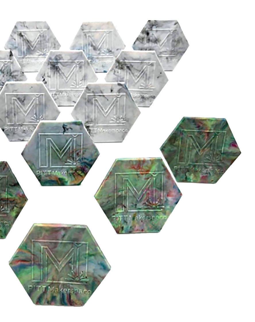
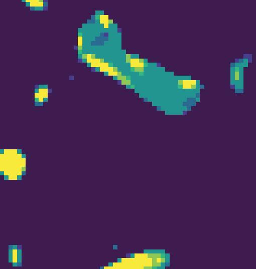
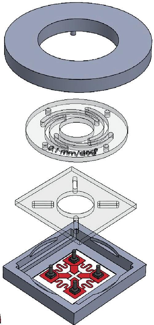
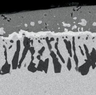
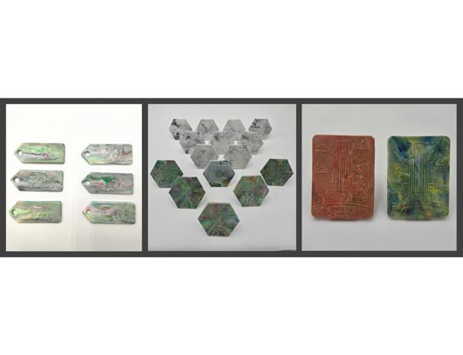
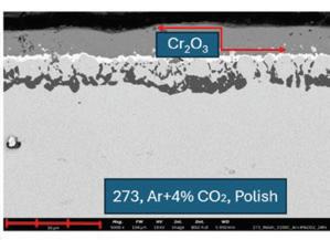
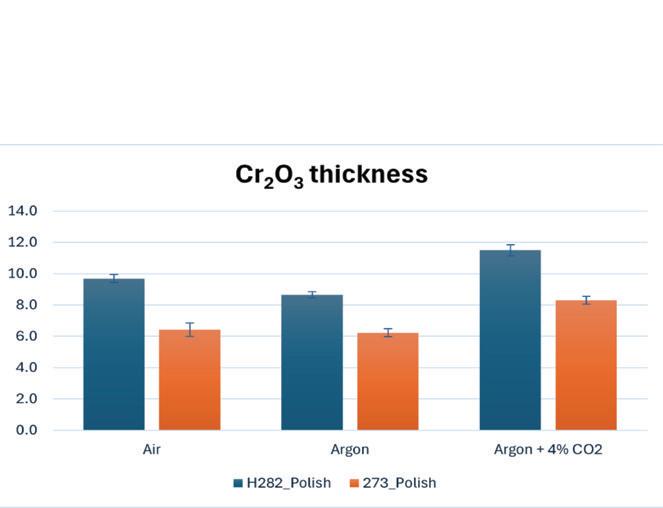
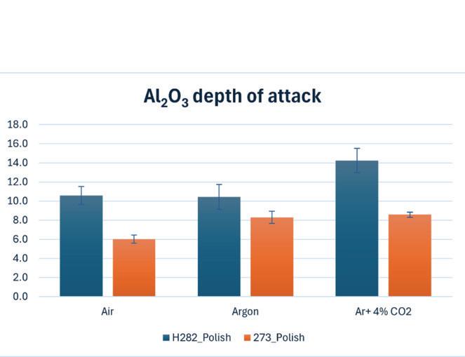
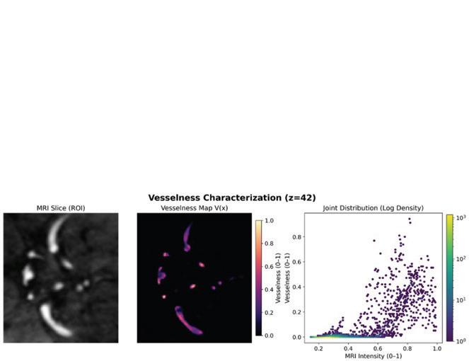
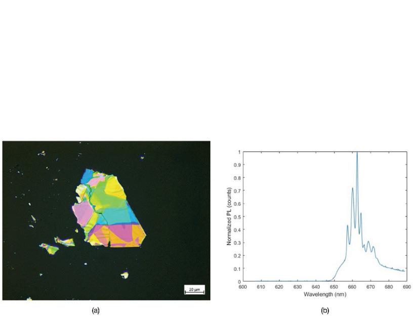
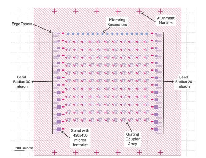
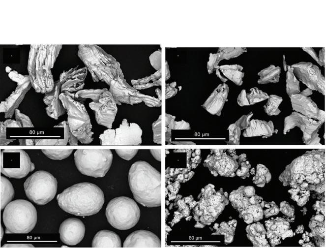
Cover images from left to right, top half then bottom half: Hexagonal injection-molded tiles produced from recycled PLA plastic (See page 8 by Brenna M. Baker, Ethan J. Bell, and Miles Rosas), MRI vesselness characterization map of cerebral vasculature (See page 48 by Isaiah Jefferson), an exploded CAD schematic of the EquuStretch biaxial tissue stretcher system (See page 57 by Carter Jones), SEM cross-sections of oxide scales formed on nickel-based high-temperature alloys (See page 23 by Snigdha Garud); and continuing left to right across the bottom half: an SLA-printed resin injection mold bearing an embossed Pittsburgh skyline design (See page 8 by Brenna M. Baker, Ethan J. Bell, and Miles Rosas), SEM micrographs of spherical copper powder morphology used in binder-jet printed filters (See page 70 by Amelia Morrison), the EquuStretch biaxial tissue stretcher cassette device (See page 57 by Carter Jones), a microscopy image of an exfoliated AgErP₂Se₆ flake for photonic chip integration (See page 61 by Shriya Krishnamurthy), and SEM micrographs of binder-jet printed copper filter cross-sections at varying powder morphologies (See page 70 by Amelia Morrison).
Please note that neither Ingenium nor the Swanson School of Engineering retains any copyright of the original work produced in this issue. However, the Swanson School does retain the right to nonexclusive use in print and electronic formats of all papers as published in Ingenium
TABLE OF CONTENTS
Message from Interim Associate Dean for Research and Facilities .................................. 5 Message from Co-Editors-in-Chief ...................... 6 Graduate Student Review Board — Ingenium 2026 ................................................. 7
BAKER, BRENNA
A Low-cost, Replicable Injection Molding System for Recycling PLA Waste in Engineering Makerspaces to Support Experiential Learning ............................. 8
Advisor: William Clark — Education Research
BARPANDE, JANHAVI
Linking Local Collagen Density to Mechanical Strength in Thoracic Aortic Aneurysms ....................................................... 12
Advisor: David Vorp — Experimental Research
CLASON, KAT
Evolution of Gap Formation in Achilles Tendon Repair .................................................. 18
Advisor: Patrick Smolinski — Experimental Research
GARUD, SNIGDHA
ATI 273T™ and Haynes® 282®: Environmental Testing for Two Nibased High-temperature Alloys to Analyze Corrosion Resistance Through the Formation of Oxide Scales .......................... 23
Advisor: Brian Gleeson — Experimental Research
GORDON, ALEX
Machine Learning Potentials for Chemical Defense ........................................ 29
Advisor: J. Karl Johnson — Computational Research
HAMILTON, REAGAN
Strategies for Enhancing Intact Solar Cell Harvesting Toward Reuse in Solar Photovoltaic Systems ....................................... 33
Advisor: Paul Leu — Experimental Research
HSIA, BELL
Optimizing Adaptive Smoothing in Hippocampal Place Cells ................................... 38
Advisor: Shih-Cheng Yen — Methods Paper
HUDEC, BROOKE
A Tamoxifen-induced XBP1 Deletion Model for Studying Dysregulation in 12-hour Ultradian Rhythms................................ 42
Advisor: Bokai Zhu — Experimental Research
ILAHI, TAIMUR
Using MATLAB to Implement Neural Network Simulation for Synaptic Routing Optimizations ...................................... 45
Advisor: Inhee Lee — Computational Research
JEFFERSON, ISAIAH
Optimizing Multi-Scale Vesselness for Segmenting Cerebral Vasculature in MRI .......... 48
Advisor: George Stetten — Experimental Research
JIN, ZHENGYANG
Assessing Energy Use for Titanium Powder Production by Intensified Hydride-Dehydride (HDH) Upcycling ................. 53
Advisor: Jörg Wiezorek — Experimental Research
JONES, CARTER
The EquuStretch: A Device for Applying Custom Biaxial Strain to Tissues and Cells with Simultaneous Microscopy ................................. 57
Advisor: Lance Davidson — Device Design
KRISHNAMURTHY, SHRIYA
Designing and Building a Photonic Chip for On-Chip Amplification .......................... 61
Advisor: Nathan Youngblood — Device Design
MARSH, CONNOR
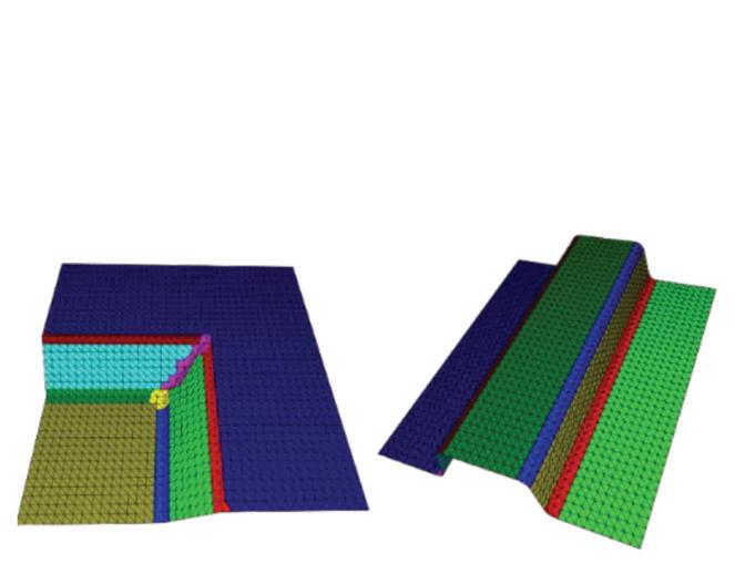
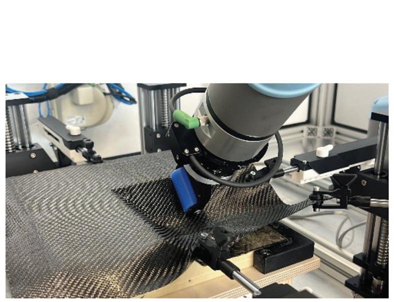
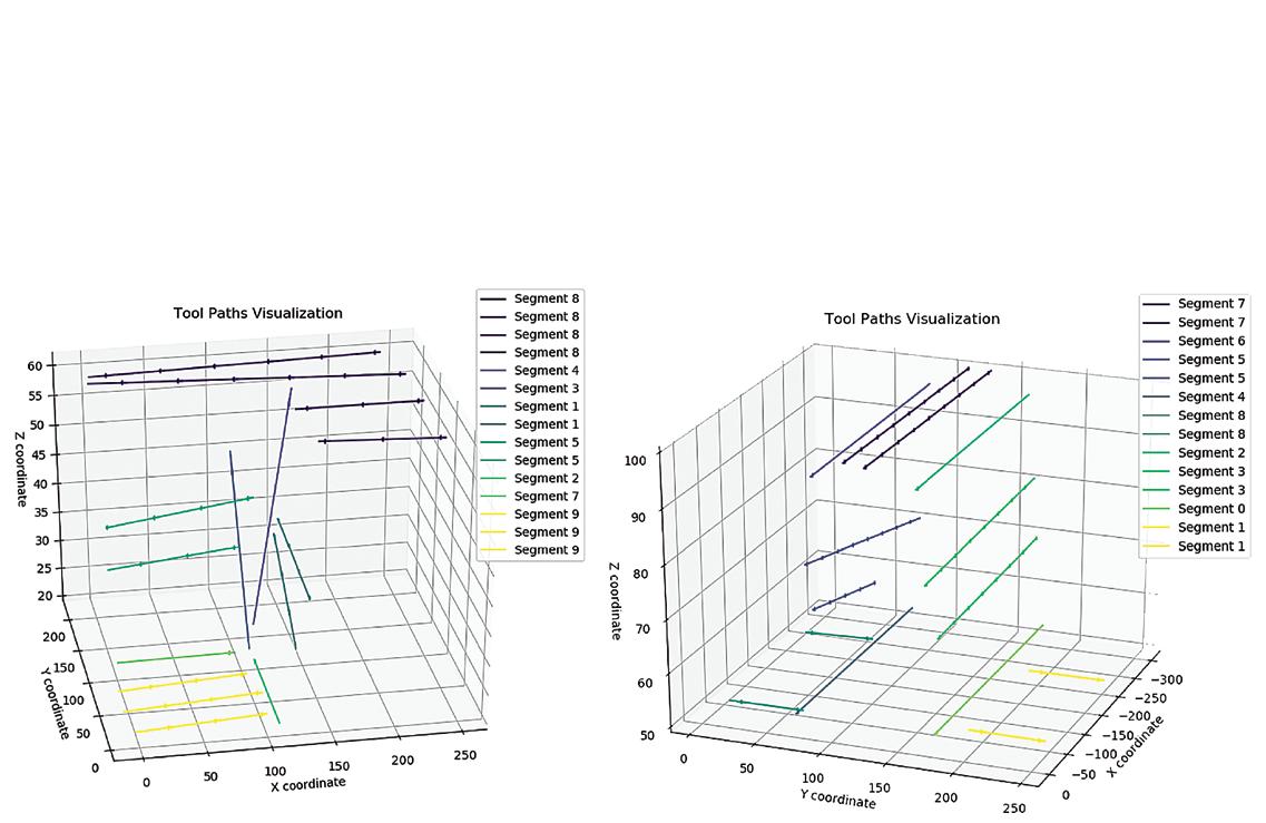
A Hybrid Trajectory Generation
Pipeline for Automated Composite Prepreg Layup using Genetic Algorithms and UV-Mapping ............................. 65
Advisor: Moritz Lennartz — Methods Paper
MORRISON, AMELIA
Optimizing Porosity as a Function of Powder Morphology in Binder-jet Printed Copper Filters ....................................... 70
Advisor: Markus Chmielus — Experimental Research
MURPHY, TRIN
Development of Small Diameter Vascular Grafts with Compliance Matching and Reduced Thrombogenicity ........... 74
Advisor: Jonathan Vande Geest — Experimental Research
NNEJI, THERESE
Comparison of Multi-scale Vesselness with Variance Wells for Segmentation of Brain Vasculature ......................................... 78
Advisor: George Stetten — Review Paper
REES, CONNOR
Mapping the Optic Nerve Connectome: A Multi-scale Imaging Approach ....................... 82
Advisor: Walter Schneider — Computational Research
SEXTON, KATHERINE
Exploring the Life Cycle Analysis of Additively Manufactured Copper Filters ............ 87
Advisor: Markus Chmielus — Review/Perspective Paper
SHAW, LOWELL
Light Management in Polymer-nanoparticle Composites .................... 91
Advisor: Jung-Kun Lee — Experimental Research
SPADAFORE, ANTHONY
Investigation on the Nonlinear Frequency-modulated Codedexcitation Pulse in Ultrasound Imaging ............. 95
Advisor: Kang Kim — Methods Paper
STONE, MADELEINE
Foundational Analysis for a Comparative LCA of PERC Monofacial vs Bifacial Solar Panels ................ 101
Advisor: Paul Leu — Computational Research
WILLIAMS, KIERSTEN
Advancing Neural Circuit Mapping: MicroCT Reveals Fasciculi and Extracellular Matrix in the Porcine Visual System .................................... 107
Advisor: Walter Schneider — Methods Paper
SWEENEY, BRYCE
Alterations in Stimulation-evoked Vascular Responses and Smooth Muscle Cell Calcium Dynamics Following Implantation of Microelectrodes in Mouse Visual Cortex .......................................112
Advisor: Takashi Kozai — Experimental Research
TRANSUE, AUDREY
Aging and Noise Exposure Interact to Cause Distinct Patterns of Cochlear Synaptopathy ................................117
Advisor: Aravind Parthasarathy — Experimental Research
WILLIAMS, ABIGAYLE
Soft Magnetic Nanocrystalline and Amorphous Alloys for Power
Electronics: Hole Defect and Thermodynamic Relationship ......................... 121
Advisor: Paul Ohodnicki — Experimental Research
WYSZYNSKI, JACKLYN
CACE Study: Harnessing
User-Input Data to Investigate Student Generative AI Usage ........................... 124
Advisor: Matthew Barry — Education Research
ZIMMERMANN, LYRIC
Harnessing 8-oxoguanine
DNA Glycosylase Activity for Mitochondrial Protection ................................. 128
Advisor: Brett Kaufman — Experimental Research
H eng Ban, PhD
A MESSAGE FROM THE INTERIM ASSOCIATE DEAN FOR RESEARCH & FACILITIES
“Ingenium” is a classical Latin noun describing a person’s innate talent and ability, particularly of the intellectual or creative variety. The naming of this publication celebrates that talent as it lives within the Swanson School, brought to life through undergraduate student research. The spark of drive and curiosity that compels young engineers to look beyond the classroom is exactly what you’ll find in the pages that follow.
On behalf of the Swanson School of Engineering and U.S. Steel Dean of Engineering Michele Manuel, I am proud to present the twelfth edition of Ingenium: Undergraduate Research at the Swanson School of Engineering. This issue showcases the accomplishments of exceptional undergraduate students through the research projects they completed during summer 2025.
As part of their undergraduate careers, students at the Swanson School may take advantage of opportunities to engage in research with a faculty mentor. Many do so through the annual Summer Undergraduate Research Internship, or “SURI” program, sponsored by the Office of Academic Affairs and the Office of the Provost. Working in labs alongside graduate students, PhD candidates, and post-doctoral scholars, they explore concepts encountered in the classroom, applying them to real-world problems and innovations. The results, represented in these pages, reflect not only technical skill, but the curiosity and persistence that define the next generation of engineers.
Upon completing their summer research, students are invited to submit a two-page abstract summarizing their results. After review and deliberation by the Graduate Student Review Board (GSRB), a select cohort is then invited to submit full manuscripts for publication. In this way, Ingenium serves as more than a record of research completed: it is also an exercise in the process of abstract submission, peer review, and scientific publication. For the graduate students who make up the review panel, Ingenium provides the opportunity to gain formal experience with the editorial process and the craft of peer review.
This edition would not have been possible without the hard work and dedication of many contributors. I would like to recognize this year’s Editors-in-Chief, Trevor Neece and May Pwint, who spent the year coordinating with the GSRB and undergraduate authors to ensure a fair, thorough, and efficient peer-review process. I am also grateful to the design team at AlphaGraphics, to Emily Huffman VonderPorten and Rose Gerber for their administrative support, and to the graduate students who committed to serve as reviewers and who are listed by name in this issue. Finally, I would like to thank the faculty mentors and coauthors whose guidance shaped the work presented here.
I hope you enjoy reading this edition of Ingenium, and that it offers you a glimpse of the future of engineering, already underway.
Hail to Pitt!
Heng Ban, PhD
Interim Associate Dean for Research & Facilities
Swanson School of Engineering University of Pittsburgh
MESSAGE FROM THE
CO-EDITORS-IN-CHIEF
Greetings!
We are excited to present the twelfth edition of Ingenium: Undergraduate Research at the Swanson School of Engineering (SSOE). Ingenium introduces undergraduate students to the scientific peer-review process, offering them the opportunity to enhance their research communication skills through the submission of written manuscripts. These manuscripts undergo review by Swanson School of Engineering (SSOE) graduate students, who volunteer to give comprehensive feedback. This process is mutually beneficial, allowing undergraduates to appreciate the reviewer’s viewpoint and gain insights into new subjects, while graduate students have the chance to impart their knowledge.
Moreover, Ingenium enables undergraduate students to engage deeply with established research methodologies through direct collaboration with PhD students and the guidance of faculty mentors. This invaluable experience prepares them for future professional endeavors, whether they aim to pursue further studies in graduate school or embark on a career in industry.
This volume features 28 articles from undergraduate students at the University of Pittsburgh’s SSOE, and students from other universities who participated in the SSOE summer undergraduate research internship program (SURI). This year’s articles show how the talents and hard work of these students provide new perspectives on relevant scientific topics being developed today. This year’s edition of Ingenium displays a sample of the diverse research that can be found in SSOE labs, and the opportunities undergraduate students are exposed to. We are so proud of all participating students for their creativity, critical thinking, hard work, and commitment to their research. We hope all authors, mentors, and reviewers share our excitement and pride and that you enjoy all the articles as much as we did!
We would like to thank everyone in the production team for this year’s Ingenium volume. We deeply thank Dr. Heng Ban, Interim Associate Dean for Research & Facilities, for his commitment to this publication. We are also extremely grateful to Emily VonderPorten and Rose Gerber, for their advice, guidance, and continued support throughout the entire year. We also deeply appreciate all the mentors who guided the students’ research and the graduate students on the GSRB, for dedicating so much of their not-so-free time and sharing their knowledge to advise the authors. Finally, we would like to thank everyone in the Office of the University Communiciations and Marketing and the AlphaGraphics team, especially Matt Miller and Mitchell Longstreth for their amazing work with the production and design of this Ingenium edition.
We have learned so much from everyone involved in this year’s Ingenium edition, and we are honored to have served as Co-Editors-in-Chief. It was truly a most rewarding experience to continue this Pitt SSOE tradition and to be part of a remarkable research community that invests in students and their academic and personal development. We hope that as you read this year’s articles, you let yourself be submerged in the wonderful research developments, as well as the passion and hard work shown by the authors.
38. Stricklin, Andrew — Mechanical Engineering & Materials Science
39. Thakkar, Shreya — Chemical Engineering
40. Twizerimana, Aime — Chemical Engineering
41. Vibhute, Chaitanya — Bioengineering
A low-cost, replicable injection molding system for recycling PLA waste in engineering makerspaces to support experiential learning
WILLIAM W. CLARK
William W. Clark, PhD is a professor of Mechanical Engineering and Materials Science where he teaches and carries out research in dynamic systems and controls. He is also the Director of the Innovation & Entrepreneurship Program in the Swanson School of Engineering that is responsible for building a community of innovation in the school.
Brenna M. Baker1†, Ethan J. Bell2†, Miles Rosas2†, William W. Clark 2
1Department of Bioengineering, University of Pittsburgh, Pittsburgh, PA
2Department of Mechanical Engineering and Materials Science, University of Pittsburgh, Pittsburgh, PA
†These authors contributed equally to this work and are considered co-first authors
BRENNA M. BAKER
Brenna Baker is an undergraduate student studying bioengineering with a focus on medical product engineering. She is currently working at a mechanical engineering co-op at MSA Safety and is pursuing the Innovation, Product Design, and Entrepreneurship Certificate. Brenna is also the Executive Secretary and CoFounder of the Injection Molding Club where she helps lead students in learning about sustainable manufacturing.
ETHAN J. BELL
Ethan Bell is a sophomore mechanical engineering student who is currently serving as an intern at the IDEA Lab, where he gains hands-on experience with design, prototyping, and manufacturing systems. He is also the President and Co-Founder of the Injection Molding Club, where he leads initiatives focused on recycling PLA waste from makerspaces into functional products through injection molding.
MILES ROSAS
Miles Rosas is a mechanical engineering student with interests in both rapid prototyping and machining skills. He is currently working as an intern at the IDEA Lab and as a student worker in the SCPI machine shop. Miles is also the Vice President and Co-Founder of the Injection Molding Club where he works to guide students through mold design and injection molding practices.
SIGNIFICANCE STATEMENT
Makerspaces often generate a significant amount of PLA (Polylactic acid) waste, but finding recycling solutions is challenging. We introduce an affordable method for transforming PLA waste into useful products using SLA (Stereolithography) printed injection molds while providing a system for sustainable education in an engineering context.
ABSTRACT
PLA is widely used in 3D printers due to its low printing temperature, biodegradability, accessibility, and ease of use. However, its popularity also means it is responsible for a large share of failed prints and waste in makerspaces. These failed parts often end up in landfills or contribute to microplastic pollution when not properly recycled. We sought to develop a sustainable method of reusing failed PLA prints using injection molding.
Conventional injection molding relies on expensive aluminum molds, making prototyping and customization inaccessible in student-led environments. To address this, we investigated the feasibility of SLA-printed resin molds. Over the course of this project, it was found that these molds can successfully be used in small-scale PLA injection molding and produce repeatable parts suitable for the creation of functional products. The goal was to reduce material waste while establishing a repeatable workflow that could be adopted in an educational setting for prototyping and sustainable manufacturing education.
Brenna M. Baker Ethan J. Bell Miles Rosas William W. Clark
1. INTRODUCTION
Globally, over 450 tons of plastic waste is produced every year, and, of that waste, almost a quarter is mismanaged [1]. That mismanaged plastic waste is not recycled and therefore ends up in landfills as environmental pollutants. University campuses produce many different types of plastic waste, and, because of this, are often looking for and finding new ways to reduce their environmental footprint. One campus location that produces significant plastic waste is makerspaces. Certain plastics are viewed as significant sources of waste in makerspaces, one main contributor being PLA. It is one of the most common materials used for prototyping and product development, particularly in 3D printing, because it is easily sourced, minimally expensive, and simple to use [2]. While convenient for rapid fabrication, unfortunately, PLA also constitutes one of the largest sources of makerspace waste. There are often cases of failed prints, unused parts, and removed support structures that all contribute to the quantity of discarded plastic. During the first semester of operation, in Benedum Hall’s makerspaces alone, the weight of discarded PLA totaled almost 20 kg. Currently, this waste is stored in large garbage bags within the workshop, consuming valuable space and leaving the material underutilized. Several ideas have been proposed to address the PLA waste in the makerspaces. Strategies included filament re-extrusion systems and centralized industrial composting programs, however, these require expensive specialized equipment, making them impractical for many student-run spaces. The objective of this project was to develop a repeatable process for reusing PLA scraps to create new, functional products while educating students about sustainable engineering practices. By implementing a structured recycling workflow, the project aimed to reduce waste and provide a model for sustainable material management. In doing so, the process was designed not only as a technical solution but also as an educational tool to provide students with resources to learn valuable engineering and manufacturing skills such as mold design and injection molding.
2. METHODS
Transforming PLA waste into new parts requires four main steps: material collection, material processing, mold design and fabrication, and injection molding.
2.1
Material Collection
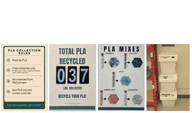
The first stage involved implementing a dedicated PLA collection system within the makerspace that would be intuitive and accessible to all who use it. Users in the space span undergraduate and graduate level students across disciplines, requiring signage to be concise and informational. The solution required a dedicated waste collection area including three stackable bins to allow PLA to be separated by color. In this area, clear instructional posters were installed, detailing what materials should be placed in the bins and how to remove any unwanted
contaminants. Additionally, highly visible signage was added in and around the collection and 3D printing area to encourage participation. These included arrows directing students to the location of the bins, a visual of different PLA shred color mixes along with their resulting injection molded part, and a modular sign showing the total quantity of PLA collected from the makerspace.
These allowed students to see where their recycled waste was going and started the conversation around the injection molding process. The implementation of the collection system formed the foundation of the material management model, ensuring consistent input for downstream processing.
2.2 Material Processing
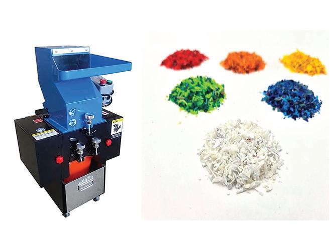
After PLA scraps were deposited in the collection bins, all material was inspected to confirm it was pure PLA and free of contaminants such as adhesives or other plastics. The verified PLA was weighed, with totals and color distribution recorded. This was a critical quality-control component in the modeled system, ensuring traceability for future optimization. The fully sorted and documented PLA was then ready to be processed into feedstock for injection molding. A plastic granulator was selected for its safety features, reliability, and ability to produce flakes approximately 5 mm in size, optimal for this project’s injection molding machine.
After one cycle of shredding, fragments were re-shredded until uniform in size and then stored according to color
Figure 1: Collection system posters and bins
Figure 2: Plastic granulator and resulting PLA shreds
category. The process was designed so future users could operate the granulator safely and easily, reinforcing the model’s focus on operational sustainability, long-term usability, and opportunity for widespread educational application.
2.3 Mold Design and Fabrication
Next, high-temperature resin molds were created using SLA printing, due to their low cost and short lead time. Approximately 3.5 molds can be produced from a single one-kilogram bottle of resin, which has a per unit cost of $60 [3]. This brings the cost per SLA-printed mold to approximately $17. Additionally, it only takes approximately 10-20 hours to print and post-process a resin mold. A standard mold is typically made of aluminum, can cost several thousand dollars, and can take weeks to be produced and shipped, as they require high-level skill and tooling that is not available at a student level [4]. This substantial cost and lead-time difference highlights the economic advantage of SLA-printed molds for rapid prototyping and low-volume production. Aluminum molds can withstand thousands of injection cycles, so mold durability of the SLA-printed molds was assessed by tracking the number of injection cycles until wear or defects appeared [2]. Mold durability testing showed that Phrozen TR300 molds maintained structural integrity for over 100 injection cycles before visible cracking or surface degradation occurred. In comparison, Siraya Tech Blu and Resione resins failed after approximately 35 and 60 cycles, respectively. These results validated the suitability of TR300 for repeated educational prototyping use. Throughout production, each molding attempt was logged, noting successful and defective parts and adjusting machine parameters to improve outcomes. These feedback loops within the process are an integral aspect of building a scalable and adaptable sustainable material management system that can effectively teach other students about the process of mold design and fabrication.
2.4 Injection Molding
Finally, the Morgan Press—a hydraulically powered injection molding machine manufactured in 1968—was used to convert PLA pellets into molded parts by clamping the mold in place and injecting molten plastic into the resin mold [5]. The goal was to produce small, durable items
suitable as gifts or promotional materials for the university, demonstrating the system’s potential to turn waste into valuable outputs. To achieve visually appealing results, shredded PLA of different colors was combined at varying ratios. Color-mixing trials were performed by molding different blends, eventually leading to a few chosen mixes including marble (black and white), Pitt (blue, yellow, and white), and confetti (multi-color and white). This process creates hands-on learning opportunities in material processing and manufacturing consistency.
3. RESULTS
With the new collection system and granulator successfully integrated into the Benedum Hall makerspace and a more thorough understanding of the injection molding process, molds were fabricated for multiple parts, including: a magnet featuring the Cathedral of Learning and the slogan “H2P”, a Pitt keychain, and a makerspacebranded tile.
Each mold produced parts with sharp details and minor post-processing needs [2]. Over a 14-week period, the 20 kg of PLA collected from the makerspace yielded roughly 1000 potential injection shots resulting in 200 functional parts. In the context of the modeled system, these outputs validated that the process could transform waste streams into desirable products, reinforcing the viability of sustainable material management on a smaller scale and the opportunity for experiential educational tools to be created. Despite some malfunctions of the Morgan Press, discussed further in Section 4, consistent functional parts were created that fully recycle PLA plastic from the makerspaces around the University of Pittsburgh.
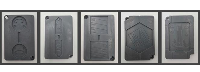
Figure 3: SLA-printed molds made from Phrozen TR300 (from left to right: pig, Pitt script keychain, IDEA Lab magnet, Makerspace magnet, and “H2P” Cathedral of Learning magnet)
Figure 4: Resulting injection molded parts made from scrap PLA (from left to right: Pitt script keychain, Makerspace magnet, and “H2P” Cathedral of Learning Magnet)
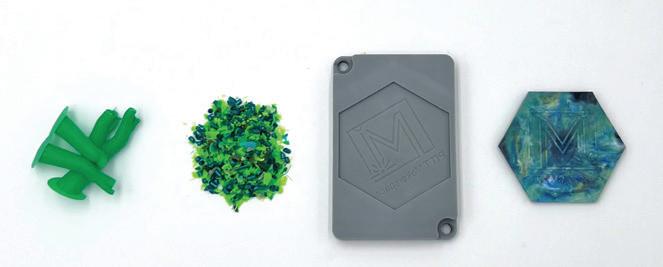
Figure 5: Four stages of PLA processing; starting with 3D print scrap and ending as an injection molded part
4. DISCUSSION
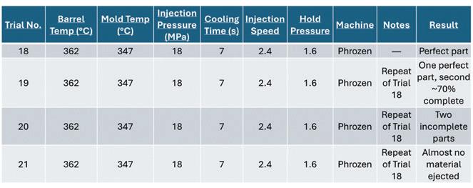
The feasibility of recycling PLA waste into functional products was established, however, key limitations arose, including the Morgan Press’s single-sided mold constraint, PLA’s potential degradation after repeated heating, and the inconsistency of the Morgan Press. While the Morgan Press successfully allowed for the recycling of PLA into functional products, the system’s ability to have broader educational impact was challenged by the machine’s inconsistent molding results. Using the same mold and settings produced a range of outcomes, including over shots, under shots, and occasional acceptable parts, which limited repeatability and increased waste.
Table 1: Results from repeated injection molding trials performed under identical processing parameters. Despite no changes to temperature, pressure, or timing settings, part quality varied significantly across trials.
Consultation with the manufacturer identified a defective timer valve and overall aging components as the cause of the machine’s inconsistency [3]. As a result, the project shifted focus toward evaluating modern desktop injection molding machines which will allow this system to have improved consistency and expanded educational use in the future.
Future work may explore two-sided molds, more durable mold resins, and purchasing an improved injection mold machine. With a new device, parts could be produced more efficiently compared to the Morgan Press results. Additionally, this improvement would make the system a stronger educational tool in classrooms around the Swanson School of Engineering because it would allow for higher-level student involvement in a process more reflective of industry standards. There is an opportunity for the practices implemented through this project to have an impact on a broader scale. Collaboration with other campus facilities or local makerspaces could further augment the system by providing resources, materials, and educational partnerships that would allow for growth outside of Benedum Hall. This modeled workflow potentially provides a pathway for other institutions to implement sustainable education-based material management practices.
5. CONCLUSIONS
This project successfully demonstrates the ability
to repeatably recycle PLA plastic in the University of Pittsburgh Makerspace by collecting, organizing, shredding, and injecting new and beneficial parts that are useful and to teach students valuable engineering practices. Implementation of this system diverted approximately 20 kg of PLA from waste streams in one semester and enabled production of over 100 functional parts. The use of SLA-printed molds made with Phrozen TR300 has proved to be a cost-effective alternative to aluminum molds. The molds can withstand many molding cycles while maintaining durability and surface quality, validating their suitability for educational prototyping. Beyond material reuse, this work highlights the educational value of integrating sustainable manufacturing practices into makerspaces. Over 50 students were directly exposed to core engineering concepts including material processing, mold design, and injection molding operations, reinforcing hands-on learning while addressing realworld sustainability challenges. Additionally, this system impacted more than 200 additional makerspace users through exposure to the recycling workflow and practices in sustainability. Overall, the developed system provides a scalable model for sustainable material management that can be readily adopted by other academic institutions seeking to reduce plastic waste while enhancing engineering education.
ACKNOWLDGEMENTS
The IDEA Lab staff, Brandon Barber, Daniel Yates, Amelia Gordon, Dr. Kevin Bell, and Dr. William Clark for their guidance and continued support throughout this project. Funding was provided by the Swanson School of Engineering and the Office of the Provost at the University of Pittsburgh.
REFERENCES
[1] H. Ritchie, V. Samborska, and M. Roser, “Plastic pollution,” Our World in Data, 2023. [Online]. Available: https://ourworldindata.org/plastic-pollution
[2] Ticona, “Designing with plastics: The fundamentals,” Scribd, n.d. [Online]. Available: https://www.scribd. com/document/253546376/Designing-With-PlasticsTicona
[5] Morgan Industries, Inc., “Morgan-Press main guide,” n.d. [Online]. Available: https://peoplevine.blob.core. windows.net/media/397/business/3624/Morgan_ Press_Main_Guide.pdf
Linking Local Collagen Density to Mechanical Strength in Thoracic Aortic Aneurysms
Janhavi M. Barpande1, Pete H. Gueldner1, Kumbakonam R. Rajagopal1,9 and David A. Vorp1-8
1Department of Bioengineering, University of Pittsburgh
2Department of Mechanical Engineering and Materials Science, University of Pittsburgh
3McGowan Institute for Regenerative Medicine, University of Pittsburgh
4Department of Surgery, University of Pittsburgh
5Department of Chemical and Petroleum Engineering, University of Pittsburgh
6Department of Cardiothoracic Surgery, University of Pittsburgh
7Clinical & Translational Sciences Institute, University of Pittsburgh
8Magee-Womens Research Institute, Pittsburgh, PA, USA
9Department of Mechanical Engineering, Texas A&M University, College Station, TX
JANHAVI BARPANDE
Janhavi Barpande is a senior undergraduate Bioengineering student at the University of Pittsburgh. Her area of focus is soft tissue biomechanics, specifically cardiovascular tissue. Currently, she works as a Research Assistant in the Vascular Bioengineering Lab with Dr. David Vorp (Swanson School of Engineering). Her project investigates how the structural makeup of the thoracic aortic wall impacts its strength and likelihood of rupture during an aneurysm. To test the effect of collagen content on the mechanical strength of the aortic wall, she designed a device that administers localized protease treatment on aortic tissue to artificially mimic the heterogeneity of collagen fibers along the aorta. Then, she subjected it to uniaxial tensile load to obtain the tissue’s mechanical strength. Her main interests are understanding tissue functions and changes in pathologies under different mechanical environments. In the long term, she wants to develop artificial tissues that mimic normal functions to treat or prevent diseases and improve patients’ quality of life.
Janhavi Barpande Pete Gueldner
David Vorp Kumbakonam Rajagopal
PETE GUELDNER
Pete Gueldner, PhD is a native of San Antonio, Texas; as an undergraduate, he received his B.S. from The University of Texas at San Antonio in Biomedical Engineering with a concentration in biomechanics. He graduated from the University of Pittsburgh in 2025 with his Ph.D. in Bioengineering (concentration in biomechanics). He is now a postdoctoral associate at Yale University. His research interests are related to vascular biomechanics and artificial intelligence, primarily investigating aortic aneurysms. He is developing a novel bubble inflation testing apparatus to mechanically characterize diseased aneurysmal tissue. More rigorous experimental testing tools can significantly improve computational models by more properly analyzing material properties and failure properties. In addition to his work in experimental mechanics, he is also interested in how artificial intelligence tools can aid with computational methods and clinical diagnosis/prognosis of aneurysms.
DAVID VORP
David Vorp, PhD is the Associate Dean for Research, Swanson School of Engineering, University of Pittsburgh. In addition, he is the John A. Swanson Professor of Bioengineering, with secondary appointments in the Departments of Cardiothoracic Surgery, Surgery, and the Clinical & Translational Sciences Institute at the University of Pittsburgh. He also serves as a Co-Director of the Center for Medical Innovation and the Director of the Vascular Bioengineering Laboratory.
The research in Dr. Vorp’s lab focuses on the biomechanics, “mechanopathobiology,” regenerative medicine, and tissue engineering of tubular tissues and organs, predominantly the vasculature. He is currently studying the biomechanical progression of aortic aneurysms by modeling the mechanical forces that act on the degenerating vessel wall.
He is developing a treatment strategy for abdominal aortic aneurysms by delivering adipose-derived mesenchymal stem cells to the periadventitial side of the aneurysm to inhibit the matrix degradation commonly seen in the disease progression and promote its regeneration. Lastly, he is designing a small diameter tissue-engineered vascular graft to treat cardiovascular diseases. Here he utilizes adipose-derived mesenchymal stem cells incorporated in a biodegradable polyurethane-based scaffold (produced by the Wagner Group) that undergoes substantial in vivo remodeling to develop a native-like blood vessel. Dr. Vorp’s research has been supported by over $10 million in funding as principal investigator, and an additional $4 million as collaborating investigator, from foundation and federal agencies, including the American Heart Association (AHA) and the National Institutes of Health (NIH). He has several patents in the field of vascular bioengineering and is a co-founder of the start-up Neograft Technologies, Inc., a company that applies technology developed in Dr. Vorp’s laboratory relating to biodegradable support for arterial vein grafts.
In 2011 Dr. Vorp was recognized with the Van C. Mow Medal from the American Society of Mechanical Engineers (ASME), was twice awarded a Pitt Innovator Award, and received the Carnegie Life Sciences Award in 2013. He served on the Executive Committee of the ASME Bioengineering Division (BED; 2006-2015), serving as ASME BED Chair from 2013-2014. Dr. Vorp was elected to the Board of Directors of the Biomedical Engineering Society (BMES) for two terms (2006-2009; 2009-2012), and served two terms as BMES Secretary (2012-2014; 20142016), an executive post. In 2012, Dr. Vorp became the first non-MD President of the International Society for Applied Cardiovascular Biology, and was re-elected for a second term in 2014. Dr. Vorp is a Fellow of ASME, BMES, and the American Institute of Medical and Biological Engineering.
KUMBAKONAM RAJAGOPAL
Kumbakonam Rajagopal, PhD joined Texas A&M in 1996, where he served as the J.M. Forsyth Chair Professor. At the time of his passing in March 2025, he was also the senior research fellow of the Texas Transportation Institute and a fellow of the Michael E. DeBakey Institute.
Dr. Rajagopal’s profound contributions to engineering science have left an enduring impact on the fields of nonlinear mechanics, material modeling, and fluid-structure interactions.
His influence extended across multiple disciplines, holding faculty appointments in mechanical engineering, biomedical engineering, chemical engineering, civil and environmental engineering, engineering technology and industrial distribution, multidisciplinary engineering, ocean engineering and mathematics.
Rajagopal was the editor-in-chief of the International Journal of Engineering Science for over 15 years, one of the
leading and top-ranked journals in the field, stepping down in December 2024. He also served on the editorial board of over 10 journals, further cementing his role as a thought leader in engineering and applied mechanics.
SIGNIFICANCE STATEMENT
Mechanical strength varies due to uneven distribution of collagen fibers in aortic tissue. The goal of this study is to understand how the amount of collagen content affects the mechanical strength of aortic tissue and link it to the likelihood of rupture in thoracic aortic aneurysms in areas with reduced collagen content.
ABSTRACT
Tissue strength can vary locally due to uneven collagen fiber distribution in TAAs. Areas with lower collagen content may be less able to withstand mechanical stress and more prone to failure. To test whether aortic mechanical strength depends on local collagen content, we treated defined tissue regions with collagenase or a sham solution to mimic the heterogeneity of the aorta tissue and link it to rupture risk in low-collagen areas. Tissue was looped through a watertight well plate exposing an isolated area to collagenase or PBS treatment. Each tissue sample underwent uniaxial tensile testing. Longitudinally, 10/15 collagenase-treated samples failed at the treatment location whereas 2/15 failures occurred in the treatment region of sham-treated samples, suggesting that collagenase had an observable effect on local tissue strength and failure. There was a decrease in tensile strength for collagenase treated samples and no difference in stiffness. Circumferentially, 4/15 failures occurred in the collagenase treatment location and 2/15 failures occurred in the treatment region of sham-treated samples, suggesting that collagenase had no effect on the circumferential tissue strength and failure point. In conclusion, varying collagen content along the aneurysm tissue creates local weaknesses leading to an increased likelihood of thoracic aortic aneurysm rupture.
TAAs are most prevalent in patients over the age of 65 [1]. TAAs are the 13th most common cause of death in the United States [1]. Most of the time, TAAs are asymptomatic and go undetected until they are discovered coincidentally or dissect/rupture. Dissection occurs when pressure-induced wall stress exceeds wall strength. Aortic aneurysms are a permanent enlargement of the aorta, usually coincident with a loss of structural integrity of the aortic wall. Specifically, thoracic aortic aneurysms (TAAs) occur in the thoracic region of the aorta, superior to the diaphragm. TAAs are classified as aneurysmal when the diameter permanently increases by 50% of the original size.
The aortic wall consists of 3 layers: the innermost is the intima, the middle layer is the media, and the outermost layer is the adventitia. One of the primary structural fiber proteins in the thoracic aorta is fibrillar collagen, which primarily provides strength. Collagen is abundant in the adventitia and present in the media, making the tissue stronger and stiffer. It has been shown that the aorta has a greater stiffness and strength in the circumferential direction than in the longitudinal direction [2]. This has to do with the direction that the collagen fibers are loaded and how that alters the tissue’s mechanical properties. Previously, our group treated longitudinally oriented samples homogeneously with either elastase, collagenase, or a sham solution (phosphate-buffered saline, PBS) to understand which protein contributes to tissue strength and stiffness relative to bulk material density. Each tissue sample was treated homogeneously with either protease solution. It was found that proteolytically degrading aortic tissue lowers the bulk density and overall strength of the tissue [3].
However, tissue strength can vary locally due to the uneven distribution of collagen fibers. Ruddy et al examined regional heterogeneity within the aorta and found that different regions of the aorta contain varying levels of collagen contributing to differences in stiffness and greater susceptibility to aneurysm formation [4]. This paper suggests that aneurysmal aortic tissue may contain local areas of low collagen fiber content. Such areas may be less able to withstand mechanical stress and be more prone to rupture in that region. In our study, we test this by treating predetermined regions of the intimal aortic tissue with collagenase or a sham solution to artificially mimic heterogeneous conditions in the aneurysm bulge. The collagenase enzyme solution will degrade the collagen fibers in the treated area only, reducing its collagen content from the rest of the tissue. This approach allows us to study whether failure is more likely to occur in areas with reduced collagen content and whether aneurysms are more likely to rupture in areas with reduced collagen content. We hypothesize that sections with lower collagen fiber density, induced from collagenase treatment, will fail in regions that were treated with collagenase and at lower stresses during
mechanical testing. We also hypothesize to see a higher overall strength and stiffness in circumferentially oriented tissue due to its anisotropic nature. This may result in fewer failures seen in the collagenase treatment region of circumferentially oriented tissue. If confirmed, this would suggest that the mechanical strength of aortic tissue depends primarily on local collagen fiber content and aortic aneurysms are more prone to rupture in areas with reduced collagen content.
2. METHODS
Porcine Aorta Collection and Preparation
15 porcine thoracic aortas were collected from a local abattoir (Thoma Meat Market, Saxonburg, PA) within 24 hours of sacrifice. All pigs were 6-9 months old male Yorkshires weighing around 300 pounds. The aortas were transported to the laboratory on ice to prevent degradation. Once ready for testing, the aorta was separated from the rest of the tissue and cut open longitudinally to expose the lumen. Excess fatty tissue was cleaned. A 3D printed (using Guider II printer (Flashforge, Zhejiang, China)) die stamp was used to cut out individual specimens [5]. Flexible barber blades (Derby Professional, Newton Center, MA) were clamped inside the stamp to cut dumbbell-shaped tissue sections. Each specimen had a 60 mm total length, 40 mm gauge length, 4 mm width in the central region, and 10 mm head width on either end. Specimen thickness varied from 1 to 2 mm. Each aorta was cut into two longitudinal and two circumferential sections from the same position, avoiding damaged areas or vertebral arteries. A notch was cut into the superior edge of the sample, in the right corner facing from the intimal side to establish orientation. Each specimen was stored in PBS overnight, for an average of 16 hours at room temperature to allow for tissue saturation. Then, each orientation was treated with either sham (negative control) or collagenase treatments to artificially reduce the collagen content and mimic the heterogeneity of the aorta tissue.
Administering Protease Treatments
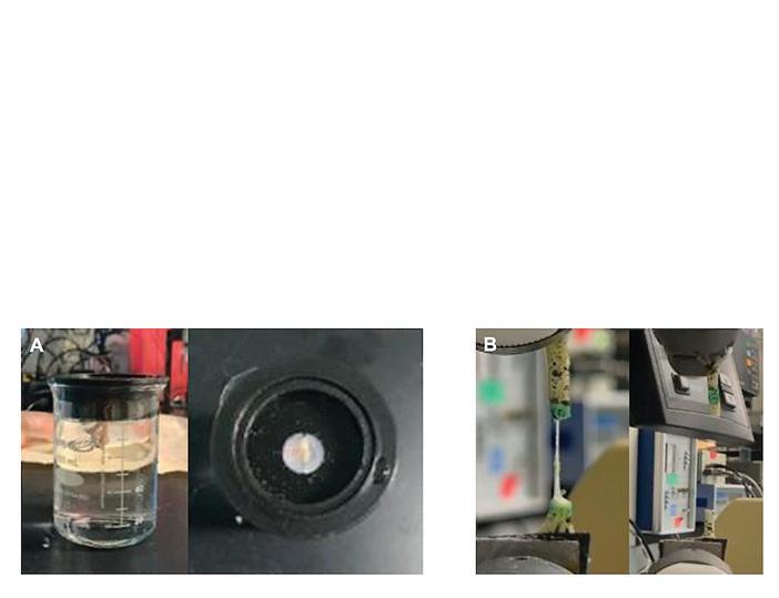
One sample from each orientation (circumferential and longitudinal) was subjected to collagenase treatment, while the other was subjected to sham (PBS) treatment. 20 mL of a 0.66 mg/mL type Ⅲ collagenase solution (Worthington, Columbus, OH) was prepared. An equal volume of PBS was measured in another beaker. Two drops of food coloring were added to both treatment solutions to stain the location of treatment on the tissue. To administer localized treatment, a well plate was designed and 3D printed (Guider II printer (Flashforge, Zhejiang, China)) with openings at the bottom through which the tissue could be looped. This raised the center of the tissue on a small bar, isolating it from the rest that hangs below in a beaker with PBS. The holes were made watertight with silicone flaps. One specimen from each orientation was looped into the well plate with the intimal
side up. The treatment solutions were poured into the well, exposing the center raised section of the tissue looped in
Experimental Set-up. A) Tissue looped through well-plate for administering localized protease treatment. B) Collagenase treated sample failed in treatment area (left) and sham treated sample failed in non-treatment area (right).
Mechanical Testing
Each sample was subjected to a uniaxial tensile test within 48 hours of harvest using an Instron uniaxial tensile tester (5543A, Norwood, MA). The Instron had a 25 N load cell with 0.01 mN resolution, and displacement was measured as grip-to-grip distance with a resolution of 0.02 mm. Each sample’s head region on either end was clamped, making sure only the center gauge length was subjected to tension. The gauge length and width, optically measured with an in-plane ruler, were 30 mm and 4 mm, respectively. Raw force vs. displacement data were collected at a constant displacement rate of 9 mm/ min until failure. The data was analyzed using a MATLAB (v R2022a, MathWorks, Natick, MA) script. Ultimate tensile strength was calculated as the maximum stress the tissue endured before failure. Stress was determined as the force recorded by the load cell divided by the tissue’s cross-sectional area determined by multiplying thickness and width in the MATLAB script. Tangent modulus was calculated as the slope of the high stretch region of the stress/strain curve before the peak or ultimate stretch. Strain was determined by the amount of stretch. Location of failure (whether it was in the treated region) was recorded (Fig. 1B). Failure location is the area at which the tissue was completely dissected during mechanical tests. Samples that failed at the clamps during uniaxial tensile testing were omitted from the study.
Statistical Analysis
Ultimate tensile strength and tangent modulus of collagenase-treated samples were compared to their adjacent sham-treated samples. Statistical analysis was
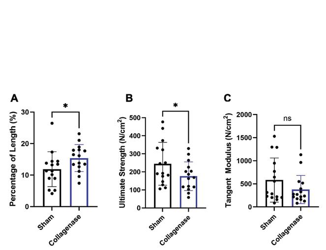
Figure 2: Tensile Test Data in the Longitudinal Orientation. A)
The percentage of length treated for each treatment (sham and collagenase) for longitudinally oriented samples. The values are statistically significant, meaning there is a change between both groups. B) The ultimate tensile strength of the tissue treated with either treatment (sham or collagenase) for longitudinally oriented samples. The values are statistically significant, meaning collagenase has an effect on tissue strength. C) The tangent modulus of the tissue treated with either treatment (sham or collagenase) for longitudinally oriented samples. The values are statistically insignificant meaning there is no major change between both groups. “*” indicates that p<0.05 and the data is statistically significant while “ns” indicates that it is not. Sample size for both groups was n=15.
performed in Prism (GraphPad, San Diego, CA) to test for normality and heteroskedasticity. Then, one-tailed t-tests were used to determine significance. The mean and standard deviation of all results were presented.
3. RESULTS
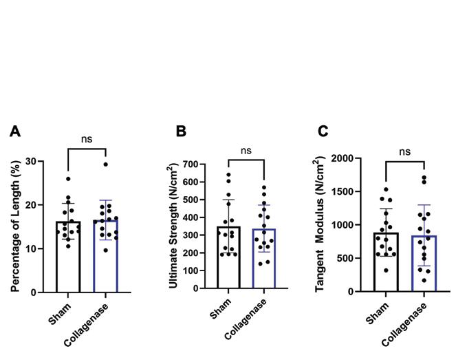
Figure 3: Tensile Test Data in the Circumferential Orientation. A)
The percentage of length treated for each treatment (sham and collagenase) for circumferentially oriented samples. The values are statistically insignificant, meaning there is no major change between both groups. B) The ultimate tensile strength of the tissue treated with either treatment (sham or collagenase) for circumferentially oriented samples. The values are statistically insignificant, meaning there is no major change between both groups. C) The tangent modulus of the tissue treated with either treatment (sham or collagenase) for circumferentially oriented samples. The values are statistically insignificant meaning there is no major change between both groups. “*” indicates that p<0.05 and the data is statistically significant while “ns” indicates that it is not. Sample size for both groups was n=15.
Figure 1:
Longitudinal Orientation:
Collagenase-treated samples had an average treatment area of 14.3±6.54 mm² (15.4±4.14% of the center surface), while sham-treated samples averaged 15.3±5.46 mm² (11.9±5.37%) (p = 0.034) (Fig. 2A). Of the collagenasetreated samples, 10 out of 15 failed at the treatment location. Two out of 15 failures occurred in the greenstained treatment region of the adjacent sham-treated samples, suggesting that the decrease in collagen fiber content due to the collagenase treatment had an observable effect on local tissue strength in contrast to samples treated only with PBS.
The ultimate tensile strength in collagenase-treated samples (175.9±76.76 N/cm2) was significantly lower than that of the sham-treated samples (244.8±114.7 N/cm2 , p = 0.036) (Fig. 2B). The tangent modulus did not significantly decrease in collagenase-treated samples (376.8±293.6 N/ cm2) compared to sham-treated samples (582.7±462.4 N/ cm2 , p = 0.08). (Fig. 2C).
Circumferential Orientation:
Collagenase-treated samples had an average treatment area of 16.0±6.07 mm² (16.6±4.37% of the center surface), while sham-treated samples averaged 17.0±5.34 mm² (16.3±3.95%) (p = 0.4) (Fig. 3A). Of the collagenase-treated samples, 4 out of 14 failed at the treatment location. Two out of 14 failures occurred in the green-stained treatment region of the adjacent sham-treated samples, suggesting that the decrease in collagen fiber content due to the collagenase treatment of circumferential samples did not have as significant of an observable effect on local tissue strength as longitudinal samples.
The ultimate tensile strength in collagenase-treated samples (349.6±144.8 N/cm2) was not significantly lower than that of the sham-treated samples (336.9±127.9 N/ cm2 , p = 0.4) (Fig. 3B). The tangent modulus was also not decreased significantly in collagenase-treated samples (884.3±345.3 N/cm2) compared to sham-treated samples (840.7±441.4 N/cm2 , p = 0.4). (Fig. 3C).
4. DISCUSSION
The longitudinally oriented samples failed at the collagenase treatment site more often (66% of the time) than those at the PBS treated site (13.3% of the time). This indicates that PBS had no effect on the tissue strength and failure point while collagenase did. Since the treated region was 11.88% of the total tissue area for PBS treated samples, statistically, we would see failure occur in the treated region at the same rate. Two out of 15 PBS treated samples broke in that area, which is 13.3%.
In the longitudinally oriented samples, the average ultimate tensile strength is significantly lower for those treated with collagenase than for those treated with PBS (Fig. 2B). In Gueldner et al., they showed a similar response where homogenously treating the tissue with collagenase reduced its ultimate tensile strength compared to tissue
treated with PBS [3]. This indicates that the collagenase treatment successfully degraded the collagen fibers, decreasing the amount of stress the tissue can sustain before failure. However, the average tangent modulus in collagenase-treated samples is not significantly lower than those treated with PBS (Fig. 2C), meaning the collagenase treatment does not have any effect on the tissue’s stiffness. We believe this is because the tissue was not treated entirely with the protease solution. Since only a small, localized area was treated, it is not large enough to cause alterations in the bulk stiffness of the tissue. Since only the collagen fibers in that area are degraded, the lower local tangent modulus made that area more prone to deformation and failure. We believe that is why there are more failures occurring in that region as that is where the failure is initiated.
We observe that longitudinally oriented collagen fibers exhibit a lower average ultimate tensile strength and tend to fail more at areas with reduced collagen content, in contrast to circumferentially oriented fibers (Fig 2B & 3B) [6]. The collagenase treated samples fail only 26.67% of the time and the sham treated samples fail 13.3% of the time in the treated area which suggests that there is not as significant of an effect on the location of tissue failure due to protease treatment. The average ultimate tensile strength and tangent modulus in the collagenase treated samples of the circumferential direction did not decrease as much as those in the longitudinal direction. This confirms the fact that circumferentially oriented tissue fibers are stronger and able to endure a greater amount of stress than longitudinally oriented tissue [2]. This is because the tissue is anisotropic, meaning the tissue properties are dependent on the direction of the tissue when the property was measured [7]. The direction of the collagen fibers changes when the orientation that the tissue is tested at changes because the fiber structure is a fixed material property in the tissue. The direction changes because the reference frames changes depending on how the sample is aligned with the loading direction. Due to its anisotropic behavior, collagen fibers are more likely to resist deformation when the sample is loaded in the circumferential direction [8]. In the future, we can test circumferentially oriented samples at a higher displacement rate.
Future directions are to change the location of treatment throughout the tissue. Currently, we only tested the center region; in the future we may test the tissue in the upper or lower quartile of the sample to see if location of failure is still associated with location of treatment. Another future direction is to test the tissue under biaxial conditions. Biaxial mechanical tests are more appropriate for multilayer, anisotropic tissue [9]. In this study, we treated the tissue as isotropic and conducted uniaxial tensile tests in both longitudinal and circumferential orientations separately. However, biaxial mechanical tests are a more accurate model of the aneurysmal environment, so we are subjecting both directions of the tissue to stress at the same time. We can combine biaxial mechanical
testing with digital image correlation to track the planar deformations throughout the tissue which can provide us with information on local stresses and strains [10].
5. CONCLUSION
This experiment exhibits that areas with reduced collagen content in an aneurysm are more prone to failure as they have a lower ultimate tensile strength compared to areas containing a normal amount of collagen (Fig. 2). It has been proven that collagen fibers contribute to tissue strength, so areas with fewer fibers or broken fibers are weaker. Reduced collagen content creates local areas that are unable to sustain greater amounts of stress and dissect easily. However, due to the tissue’s anisotropic nature, the properties differ based on the loading direction. We will need more data to draw conclusions about circumferentially oriented tissue.
As previously established, the aneurysmal aortic tissue is naturally heterogenous and contains areas of low collagen content which are weak and may initiate aneurysm rupture. We mimicked the heterogeneity in aortic tissue and artificially induced areas of lower collagen content by proteolytic degradation. An aortic aneurysm tissue may have such local weak points with reduced collagen content, creating regions that cannot withstand high levels of stress caused by physiological factors such as blood flow. This experiment supports the conclusion that such local regions are more susceptible to dissection, as shown by our results, and may cause sudden thoracic aortic aneurysm rupture.
ACKNOWLEDGEMENTS
We would like to acknowledge Swanson School of Engineering for funding this project through the Summer Undergraduate Research Internship. This work was supported by the American Heart Association under Grant No. 24PRE1195123 (P.H.G.) and National Institutes of Health under Grant No. R21HL181549 (D.A.V.).
REFERENCES
[1] M. A. Zafar, J. F. Chen, J. Wu, Y. Li, D. Papanikolaou, P. Charilaou, A. Elefteriades and the Yale Aortic Institute Natural History Investigators, “Natural history of descending thoracic and thoracoabdominal aortic aneurysms,” The Journal of Thoracic and Cardiovascular Surgery, vol. 161, no. 2, pp. 498–511, Feb. 2021.
[2] C. Noble, N. Smulders, N. H. Green, R. Lewis, M. J. Carré, S. E. Franklin, S. MacNeil, and Z. A. Taylor, “Creating a model of diseased artery damage and failure from healthy porcine aorta,” Journal of the Mechanical Behavior of Biomedical Materials, vol. 60, pp. 378–393, 2016.
[3] Pete H. Gueldner, Cyrus J. Darvish, Isabelle K.M. Chickanosky, Emma E. Ahlgren, Ronald Fortunato, Timothy K. Chung, Keshava Rajagopal, Chandler C. Benjamin, Spandan Maiti, Kumbakonam R. Rajagopal, and David A. Vorp, “Aortic tissue stiffness and tensile strength are correlated with density changes following proteolytic treatment,” Journal of Biomechanics, Volume 172, 2024.
[4] J. M. Ruddy, J. A. Jones, F. G. Spinale, and J. S. Ikonomidis, “Regional heterogeneity within the aorta: relevance to aneurysm disease,” The Journal of Thoracic and Cardiovascular Surgery, vol. 136, no. 5, pp. 1123–1130, Nov. 2008, doi:10.1016/j.jtcvs.2008.06.027.
[5] S.J. Nelson, J.J. Creechley, M.E. Wale, and T.J. Lujan, “Print-A-Punch: A 3D printed device to cut dumbbellshaped specimens from soft tissue for tensile testing,” J. Biomech., 112 (2020), Article 110011.
[6] G.V. Guinea, J.M. Atienza, F.J. Rojo, C.M. GarcíaHerrera, L. Yiqun, E. Claes, J.M. Goicolea, C. GarcíaMontero, R.L. Burgos, and F.J. Goicolea, “Factors influencing the mechanical behaviour of healthy human descending thoracic aorta,” Physiol. Meas , 31 (2010), p. 1553.
[7] Liu, L. Liang, F. Sulejmani, X. Lou, G. Iannucci, E. Chen, B. Leshnower, and W. Sun, “Identification of in vivo nonlinear anisotropic mechanical properties of ascending thoracic aortic aneurysm from patient-specific CT scans,” Sci. Rep., 9 (2019), p. 12983.
[8] X. Wang, H. J. Carpenter, M. H. Ghayesh, A. Kotousov, A. C. Zander, M. Amabili, and P. J. Psaltis, “A review on the biomechanical behaviour of the aorta,” J ournal of the Mechanical Behavior of Biomedical Materials, vol. 144, p. 105922, Aug. 2023, doi:10.1016/j. jmbbm.2023.105922.
[9] Jumpei Takada, Kohei Hamada, Xiaodong Zhu, Yusuke Tsuboko, and Kiyotaka Iwasaki, “Biaxial tensile testing system for measuring mechanical properties of both sides of biological tissues,” Journal of the Mechanical Behavior of Biomedical Materials, Volume 146, 2023.
[10] Hutomo Tanoto, Zhongxi Zhou, Kaijia Chen, Riuxin Qiu, Hanwen Fan, Jacob Zachary Chen, Ethan Milton, Yuxiao Zhou, and Minliang Liu, “Predicting biaxial failure strengths of aortic tissues using a dispersed fiber failure model,” Extreme Mechanics Letters, Volume 75, 2025, 102287.
Evolution of Gap Formation in Achilles Tendon Repair
Kat Clason1, Conor Fallon1, Shoichi Hattori2 , William Gamble1, Patrick Smolinski1 and Macalus Hogan2
1Department of Mechanical Engineering and Materials Science, University of Pittsburgh
2Department of Orthopedic Surgery, University of Pittsburgh
KAT CLASON
Kat Clason is from Orwell, OH, and is currently a BS degree student in the Department of Bioengineering, with a minor in Mechanical Engineering. She has an interest in orthopedic device development and design.
CONOR FALLON
Conor Fallon received his B.S. in Mechanical Engineering from the University of Pittsburgh. His interests include mechanical design and medical device technologies. He plans to pursue a career in intellectual property law, focusing on the protection and development of innovative technologies.
WILL GAMBLE
Will Gamble is a third year graduate student in the mechanical engineering and material science department. He received his bachelor’s degree in mechanical engineering from Pitt, and plans to pursue a PhD with a focus of biomechanics. Will’s research interests include the modeling strain lower limb joints and studying the mechanics of the legs.
PATRICK SMOLINSKI
Patrick Smolinski has a Ph.D. in Theoretical and Applied Mechanics from Northwestern University. His lab is interested in the joint injury mechanics, tissue mechanical properties and the mechanical evaluation of surgical treatments in orthopaedics and sports medicine.
SOICHI HATTORI
Soichi Hattori received his M.D. from the Keio University School of Medicine in Tokyo, where he also completed his residency in orthopaedic surgery. He performed a fellowship in foot and ankle surgery at the University of Pittsburgh Medical Center. His clinical and research interests include orthopaedic trauma, foot and ankle reconstruction, and sports medicine..
MACALUS V. HOGAN
MaCalus V. Hogan earned his M.D. from the Howard University College of Medicine and completed his residency in orthopaedic surgery at the University of Virginia Health System. He also completed a fellowship in foot and ankle surgery at the Hospital for Special Surgery. His clinical and research focus includes sports-related foot and
ankle injuries, dance medicine, and the development of regenerative medicine therapies for musculoskeletal health.
STATEMENT OF SIGNIFICANCE
The knowledge of how Achilles tendon repairs resist gap formation and growth under cyclic loading is not well known. This study will provide information that can help determine which repair best resists gapping which will allow better rehabilitation and healing.
ABSTRACT
Achilles tendon ruptures are a common injury, and surgical repair is typically recommended. Although multiple suture techniques exist, it remains unclear which method best resists gapping at the repair site. Identifying the most effective technique could improve healing outcomes and accelerate rehabilitation. This study compared 2-strand and 4-strand Krackow suture repair methods to determine which demonstrated superior performance under cyclic loading. Tendon gapping (mm) was measured after 100, 200, 300, 400, and 500 loading cycles using a MTI-5K (MTI, Inc.) testing machine. It was hypothesized that the 4-strand Krackow technique would exhibit significantly less gapping than the 2-strand Krackow technique. The results showed that the 4-strand repair had significantly less gapping at all measured cycles compared to the 2-strand repair, rejecting the null hypothesis. Clinically, these findings suggest that use of a 4-strand Krackow repair may better maintain tendon apposition during early rehabilitation loading.
Category: Experimental Research; Cadaveric Study; Literature Review
Keywords: Achilles tendon repair, cyclic loading, gap formation
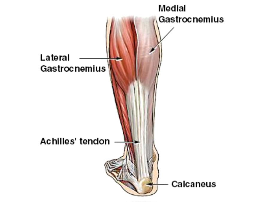
The Achilles tendon connects the soleus muscle and the medial and lateral gastrocnemius muscles to the calcaneus.
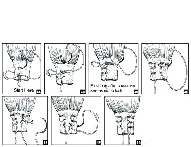
Many types of repair techniques exist; however, a common type of suture repair is the Krackow technique. The Krackow technique is a continuous locking loop suture technique that can involve a variable number of sutures (Figure 2) [6].
Figure 1: Location of the Achilles Tendon Schematic (specialtyorthony.com).
Although the Achilles tendon is the largest and longest tendon in the body, ruptures of the Achilles tendon are still common, with an incidence of approximately 18 per 100,000 people per year [1]. Surgery is typically recommended for Achilles tendon ruptures, as nonsurgical recovery is generally reserved for older populations and is associated with a longer recovery time and a greater risk of re-injury. There are multiple different techniques to repair an Achilles tendon injury, but the most common is to suture the rupture back together [1].
With repair, suture techniques can differ in their configurations, which may influence the biomechanical properties of the tendon after the repair, including strength and gap formation at the repair site [1,6]. Reducing tendon elongation and gap formation in early rehabilitation has been proven to improve patients’ Achilles Tendon Total Rupture Scores (ATRS), which is a patient-reported instrument for measuring the outcomes after treatment for Achilles tendon rupture [2]. Therefore, understanding the evolution of gap formation during early cyclic loading is critical for optimizing repair strategies. By evaluating how gap formation and elongation evolve under repetitive loading conditions, this study aims to provide insights into the comparative biomechanical performance of two repair techniques.
Studies of Achilles tendon repair techniques have shifted toward evaluating cyclic loading to better reflect early rehabilitation conditions. In 2006, Lee and colleagues compared a 4-strand Krackow, an augmented 4-strand Krackow, and a percutaneous [3]. Van Dyke et al. (2017) compared gapping between the Bunnell technique and the Giftbox repair [4]. Tian et al. (2019) compared LindholmModified Bunnell-Krackow (LMBK) and Giftbox repairs in bovine tendons across two staged loadings [5]. Comparing the findings from each of these studies highlight ongoing variability in repair performance and underscore the need for further comparative evaluation under cyclic loading conditions. Despite these findings, there remains limited comparative evidence specifically evaluating different Krackow configurations under cyclic loading.
The objective of this study is to quantify and compare gap formation after 100, 200, 300, 400, and 500 cycles of tensile loading in Achilles tendon repairs using both 2-strand and 4-strand Krackow suture configurations. The hypothesis is that the 4-strand suture will have a smaller gap formation than the 2-strand. To obtain precise measurements of the gap, digital image correlation (DIC) images will be captured at each interval to assess deformation. This analysis will provide data on the progression of gap formation under cyclic loading and help inform surgical technique selection for Achilles tendon repairs.
2. METHODS
Specimen Preparation
Prior approval was granted for this research study by the Committee for Oversight of Research and Clinical Training Involving Decedents (CORID #1186). The cadaveric specimens were procured from institutionally approved tissue suppliers. All specimens were stored in freezers at 0°F and thawed at room temperature for 24 hours before dissection. During dissection, the Achilles tendon
Figure 2: Krackow Repair Procedure [6].
was identified, checked for any injuries and severed 6 cm proximal from insertion in the calcaneus. The specimens were random assigned to either the 2-strand Krackow or the 4-strand Krackow repair group and the assigned repair was performed on the rupture. Seven specimens (55.1 ± 7.5 y) underwent 2-strand Krackow repair and 8 specimens (mean age: 63.3 ± 14.3 y) underwent 4-strand Krackow repair.
All repairs were performed by an orthopedic surgeon named Dr. Shoichi Hattori. Specimens were not paired which is a limitation of the study.
Once the repair was completed, the tendon was transected 14 cm proximal of insertion site, and a calcaneal bone block extracted distally to the insertion. The tendons were not dog-boned prior to testing.
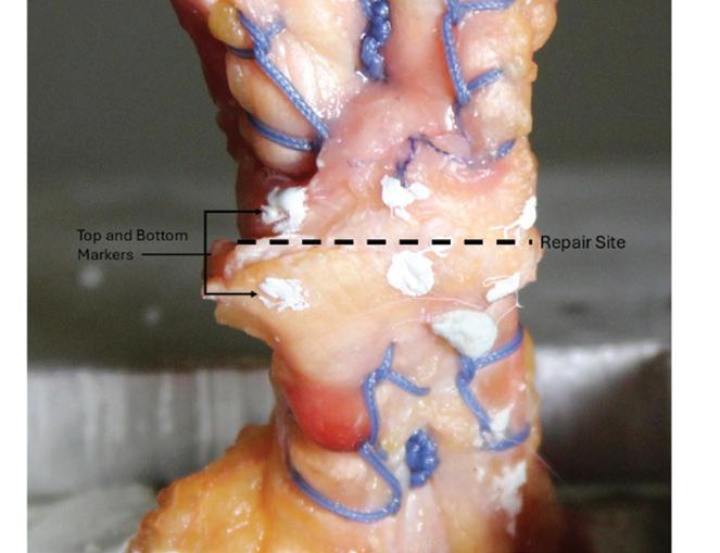
The calcaneal bone block was then potted in polymer resin while ensuring the tendon insertion was exposed. Six white dots were drawn on the tendon using paint both immediately above and below the repair site. The white dots were placed on the left edge, middle, and right edge of the repair, as close as possible to the rupture (figure 3).
This was done to freeze the tissue and prevent slip in the grip during loading. The distal resin bone block was rigidly clamped underneath a flat metal plate fixture.
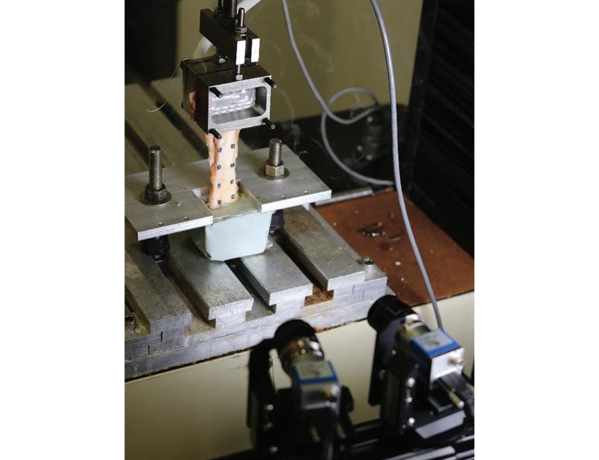
A digital image correlation (DIC) (Correlated Solution Inc.) optical tracking system was set up racing the specimen with clear view of the white dots. This system consisted of two cameras and a light used to capture a video of the specimen during loading (figure 5).
The video system (VIC-3D Digital Image Correlation) tracked the markers during loading to measure the separation of the tissue (gap) during testing.
Axial Loading
The tendon specimen was secured at both ends in the material testing machine (MTI-5K, MTI, Inc.) to apply uniaxial tensile loading. The proximal end of the tendon was clamped using a freeze-clamp cooled by liquid nitrogen repair (figure 4).
The cameras captured video at a frame rate of 250 ms. The camera system was calibrated prior to specimen loading.
All tendons underwent 500 cycles of loading ranging from 20 to 100 N at a rate of 2 Hz [4,5]. The video recorded during loading was uploaded and analyzed using the VIC3D (Correlated Solutions, Inc.) software to measure the
Figure 3: Close up of a repair Achilles tendon with the left, middle, and right white markers.
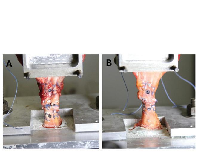
Figure 4: (A) 4-strand Krackow repair unloaded. (B) 2-strand Krackow repair mounted in testing system. The tissue is unloaded.
Figure 5: The testing set-up.
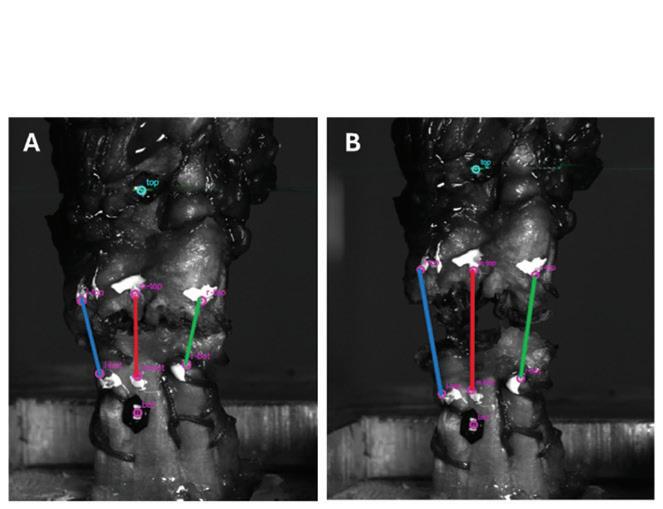
initial (without load) distance (L o) and loaded distance (L) between the markers. VIC-3D allows manual tracking of the location coordinates of the markers on every frame of the video.
These location values can then be exported to Microsoft Excel for calculation of the distance between the dots above and below the repair at each location. The difference in the distance between the markers from the unloaded state (L ) and loaded state (L) is defined as the gap. The gap was measured at the left, middle and right marker locations progressively at 100, 200, 300, 400 and 500 cycles. Since the first measurements were taken after 100 loading cycles, no preconditioning was deemed necessary as in a previous study [3],
Statistical analysis was performed to assess differences in data. A two-way Anova found there was no significant difference in gap location but there was a significant difference between repair method. The left, center, and right gaps were averaged to compute a mean gap at each cycle. The primary outcome measure was mean gap formation (mm) at each cycle interval (100, 200, 300, 400, and 500 cycles).
A one-sided t-test was performed at each cycle interval to compare mean gap formation between the two repair methods (2-strand vs. 4-strand), under the a priori assumption that the 4-strand Krackow repair would result in smaller gap formation than the 2-strand repair, consistent with the stated hypothesis. Significance was taken as p<0.05.
3. RESULTS
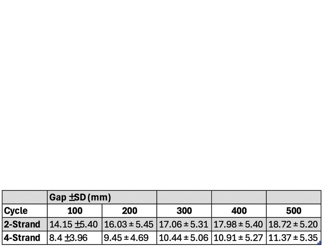
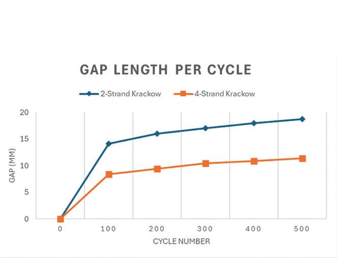
Figure 7 shows the mean of left, center, and right gaps for each of the two repair techniques. The mean gaps, average of the left, right, and middle gap measurements, at the different cycles for the two methods are given in Table 1. For both repair techniques, mean gaps increased progressively with the number of cycles. At every cycle, the 4-strand repair demonstrated significantly smaller gaps than the 2-strand repair (p<0.05).
For the 2-strand Krackow repair, the mean gap increased from 14.15 mm at 100 cycles to 16.03 mm at 200 cycles, 17.06 mm at 300 cycles, 17.98 mm at 400 cycles, and 18.72 mm at 500 cycles. In comparison, the 4-strand repair exhibited smaller mean gaps, increasing from 8.40 mm at 100 cycles to 9.45 mm at 200 cycles, 10.44 mm at 300 cycles, 10.91 mm at 400 cycles, and 11.37 mm at 500 cycles.
Figure 7: Comparison of the gap length (mm) between the 2-strand and 4-strand repairs at regular 100-cycle intervals.
Table 1: The average values of the gap measurements in mm of the two repair types at the 100th, 200th, 300th, 400th, and 500th cycle. All values of the two repair methods were significantly different at all cycles.
Figure 6: (A) Unloaded specimen and (B) Loaded specimen showing the initial distance between the markers at the left (blue), middle (red), and right (green).
4. DISCUSSION
The most important finding of this study was that the 4-strand suture Krackow repair developed significantly smaller gaps than the 2-strand suture Krackow repair under 500 loading cycle history. The one-sided t-test was applied after each 100 loading cycles to test the hypothesis that the 4-strand repair would have smaller gaps than the 2-strand repair, rather than comparing sequential cycles within a repair.
In the study conducted by Van Dyke, the gapping found after 500 cycles in the Giftbox and Bunnel repairs was smaller than in the Krackow repairs tested in this study [4]. Similarly, Tian et al., using bovine tendons, reported that the LBMK and Giftbox techniques demonstrated less gapping than Krackow repairs after 500 loading cycles [5]. Although these findings suggest that both the 4-strand and 2-strand Krackow repair methods may be inferior to alternative repair techniques, direct comparisons should be made with caution. Differences in loading protocols and gap measurement methods across studies may have influenced the reported results.
There are several limitations of this study. First, specimens were not paired, meaning donor-specific variability could influence the results, however, independent samples were assumed in the statistical analysis. Second, no dog-boning of the tissue was performed, meaning the test samples could have different cross-sectional areas. However, in creating the injury the tendon was fully transected and thus the specimen strength and stiffness was mainly a function of the sutures since no load could be transferred across the injury by the tissue. This approach preserves natural tendon geometry, better representing clinical repair conditions and has been used in the previous studies. Finally, the sample size was relatively small, although statistically significant differences were observed at all cycle intervals.
Future studies could examine additional suture configurations or explore variable rehabilitation loading protocols to optimize clinical recommendations. Investigating paired contralateral specimens or larger sample sizes would strengthen the statistical power and account for donor-specific variability.
5. CONCLUSION
This study quantified and compared gap formation in 2and 4-strand Krackow Achilles tendon repairs under cyclic loading. The major finding was that the 4-strand Krackow repair consistently exhibited significantly smaller gaps at all 100-cycle intervals (100-500 cycles), rejecting the null hypothesis.
This study shows that the additional supply and operating room costs for the 4-strand Krackow repair are justified by its improved load bearing performance. This may result in quicker recovery times, with fewer complications, thus improving patient outcomes.
Overall, this study supports the initial aim of determining which Krackow configuration better resists gapping and provides actionable guidance for surgical decision-making in Achilles tendon repair.
[2] Yassin, Mohamed et al. “Does size of tendon gap affect patient-reported outcome following Achilles tendon rupture treated with functional rehabilitation?.” The Bone & Joint Journal, vol. 102-B,11 (2020): 1535-1541. doi:10.1302/0301-620X.102B11. BJJ-2020-0908.R1
[3] Lee, Steven J et al. “Cyclic loading of 3 Achilles tendon repairs simulating early postoperative forces.” The American Journal of Sports Medicine, vol. 37,4 (2009): 786-90. doi:10.1177/0363546508328595
[4] Van Dyke, Rufus O et al. “Biomechanical Head-toHead Comparison of 2 Sutures and the Giftbox Versus Bunnell Techniques for Midsubstance Achilles Tendon Ruptures.” Orthopaedic Journal of Sports Medicine, vol. 5,5 2325967117707477. 30 May 2017, doi:10.1177/2325967117707477
[5] Tian, Jian et al. “Achilles tendon rupture repair: Biomechanical comparison of the locking block modified Krackow technique and the Giftbox technique.” Injury, vol. 51,2 (2020): 559-564. doi:10.1016/j.injury.2019.10.019
[6] Krackow, Kenneth A. “The Krackow suture: how, when, and why.” Orthopedics, vol. 31,9 (2008): 931-3. doi:10.3928/01477447-20080901-19
ATI
273 TM and
Haynes® 282®: Environmental testing for two Ni-based hightemperature alloys to analyze corrosion resistance through the formation of oxide scales
Snigdha Garud, Jonathan Locker, Brian Gleeson
Department of Mechanical Engineering and Materials Science, University of Pittsburgh
SNIGDHA GARUD
Snigdha Garud is a junior Materials Science and Engineering student at the University of Pittsburgh. Her research interests include additive manufacturing, high-temperature corrosion, and simulation design. After graduation, she plans to pursue a master’s degree in mechanical engineering and work in failure analysis.
BRIAN GLEESON
Brian Gleeson is currently the Harry S. Tack Chaired Professor of Materials Science in the Department of Mechanical Engineering and Materials Science at the University of Pittsburgh. He was the Chairman of this department from May 2014 to August 2025. Prior to taking the Chairman position in May 2014, he served as Director of the University of Pittsburgh’s Center for Energy (2008-2014). Dr. Gleeson received his degrees in materials science & engineering (MSE) from the University of Western Ontario, Canada (BE 1984; ME 1986) and the University of California at Los Angeles (PhD 1989). He was a postdoctoral fellow and then a faculty member in the MSE Department at the University of New South Wales, Australia, from 1990-1997. He moved to Iowa State University (ISU) in 1998, where, in 2006, he was appointed the Renken Professor of MSE. From 2001-2006 he also served as Director of the Materials & Engineering Physics Program at the U.S. Department of Energy’s Ames Laboratory, which is managed by ISU. In the fall of 2007, he moved to the University of Pittsburgh.
JONATHAN LOCKER
Jonathan Locker is a PhD candidate in the Department of Mechanical Engineering and Materials Science at the University of Pittsburgh, where his research focuses on how steam, CO2 , and oxygen affect the oxidation behavior of alumina and chromia forming nickel-based alloys. His work is relevant to high power generation systems such as hydrogen combustion engines which have reduced emissions compared to normal internal combustion engines which use hydrocarbon-based fuels. He has worked with GE Aerospace, Oak Ridge National Laboratory, and Brookhaven National Laboratory. From Raleigh, North Carolina, he completed his bachelor’s degree at the University of Pittsburgh and his master’s degree at Carnegie Mellon University prior to joining Dr. Brian Gleeson’s group as a PhD student.
SIGNIFICANCE STATEMENT
Above 1000°C, the corrosion resistance of ATI 273TM , a new nickel-based superalloy, is not as well-known as the state-of-the-art, nickel-based superalloy Haynes ® 282® This research will compare the behavior of ATI 273TM with the baseline provided by Haynes ® 282® at 1100°C through the analysis of protective oxide scale formation.
ABSTRACT
Over the past fifty years, traditional alloys have faced novel challenges. In today’s world, aerospace and power-generation processes happen at extremely high temperatures which corrode regular alloys. Hightemperature alloys, originally designed for strength, are now also optimized for oxidation resistance in extreme environments. Here, two superalloys come into the picture: ATI 273TM and Haynes ® 282®. Both form external Cr 2O3 oxide scales at high temperatures. However, Haynes ® 282®, the “workhorse” alloy used widely in industry, has a higher weight percentage of titanium than ATI 273TM , which reduces the former’s high-temperature corrosion resistance. ATI 273TM , a superalloy developed by ATI, contains intentional tantalum alloying to encourage formation of another oxide scale (Al2O3) which can offer effective resistance under extreme high-temperature conditions. In this project, both alloys were tested at 1100°C for 24 hours in three environments and with two surface finishes, using Haynes ® 282® as the comparison baseline. Characterization was done to identify oxide scales and their thicknesses. Unfortunately, after data
Snigdha Garud Jonathan Locker Brian Gleeson
analysis, it was determined that an external alumina scale did not form for any alloy, atmosphere, or surface condition. Possible causes include brief exposure and faster chromia formation over alumina due to competing oxidation kinetics. Nonetheless, when it came to overall corrosion resistance, ATI 273TM with a polished surface finish was the strongest contender based on Cr 2O3 scale thickness values and internal oxidation depth. Environmental data was inconclusive as it showed minimal statistical differences between two environments, so future work will focus on optimizing these along with promoting external alumina.
Oxide scale formation is the most important factor when it comes to analyzing corrosion resistance at high temperatures. In these extreme conditions, regular alloys rapidly degrade without forming any protective scales. High-temperature alloys are engineered to form a thin, stable oxide layer that is slow-growing, adherent, and protects the base metal with minimal alloy consumption [1]. As mentioned previously, ATI 273TM and Haynes ® 282® are two nickel-based, high-temperature alloys that form these protective scales. However, the effectiveness of the oxide scales formed by these alloys depends on thermodynamic and kinetic principles, as well as the scale thickness under high-temperature conditions.
Existing literature lists the nominal compositions of chromium and aluminum in Haynes ® 282® as 19 wt.% and 1.5 wt.%, respectively [2]. In ATI 273TM , the nominal compositions of Cr and Al are 19 wt.% and 2.2 wt.%, respectively [3]. Both alloys have the same weight percentage of chromium, but A273 has a higher weight percentage of aluminum than H282. At 1100°C, a Ni-CrAl ternary phase diagram shows that Al2O3 and Cr 2O3 are two protective oxide scales likely to form, based on the chromium and aluminum content in the alloys [4, 5]. Alumina scale formation is most likely to occur in A273, which lies at the border between II and III. This is due to its higher weight percentage of Al than H282.
Figure 1: Ternary phase diagram for a Ni-Cr-Al system from 1000°C to 1100°C. I: External NiO, internal Cr 2O3/Al2O3. II: External Cr 2O3, internal Al2O3. III: External Al2O3.
The Ellingham diagram in Figure 2 depicts the thermodynamic stability of various oxide scales [6]. Out of Al2O3 and Cr 2O3 , the former has a lower Gibbs free energy. This means that the reaction for an external alumina scale is more spontaneous, requiring less energy input and increasing the likelihood of the reaction proceeding to a stable state [7]. Thus, Al2O3 scale formation is more thermodynamically beneficial than Cr 2O3 at 1100°C.
Figure 2: Thermodynamic Ellingham diagram. At 1100°C (bottom axis), the Gibbs free energies (left axis) of two oxide scales are circled.
External Al2O3 formation is also kinetically advantageous. The Arrhenius plot in Figure 3 depicts the kinetic stability of various oxide scales [1]. Out of Al2O3 and Cr 2O3 , the former has a lower range of parabolic scaling constants, k p . Lower k p values correspond with slower oxidation kinetics, implying that an external alumina scale is slowergrowing and more stable than an external chromia scale.
2. METHODS
Figure 3: Kinetics - Arrhenius plot for various oxide scales. At 1100°C (top axis), the range of k p values for Cr 2O3 is highlighted in yellow and the range of k p values for Al2O3 is highlighted in red.
Since an external Al2O3 scale is more stable than Cr 2O3 , its formation is desirable. Alloy type, surface condition, and atmospheric factors influence alumina growth. Research shows adding 2.5 wt.% tantalum and keeping titanium below 1 wt.% in alloys improves environmental resistance by reducing oxide penetration [3]. Surface conditions can also make a difference. Compared to conventional polishing, grit-blasting increases defect density at the surface. Numerous defects could create more diffusion paths, accelerating aluminum, chromium, and oxygen movement to the surface and forming an external alumina scale [8]. Atmospheric conditions also play a key role: heating the alloy in a low-oxygen atmosphere like argon reduces oxygen influx but not aluminum outflux. This lowers O 2 activity at the alloy surface, decreases aluminum content, and could cause earlier external oxidation of alumina compared to environments like air or argon with 4% CO 2 [9]. Therefore, it is hypothesized that the presence of tantalum in ATI 273TM (over the lack thereof in Haynes ® 282®) along with grit-blasting and argon exposure will promote external alumina.
Six Haynes ® 282® and six ATI 273™ samples were sectioned into ~1.45 × 0.85 × 0.30 cm coupons. Three of each alloy (6 total) were polished to p1200, and six were gritblasted. Sample mass and dimensions were recorded prior to exposure. Samples were then evenly divided (Ex:- A273 Polish: Air, A273 Grit-Blast: Air, H282 Polish: Air, H282 Grit-Blast: Air) and exposed to air, argon, or argon + 4% CO₂ at 1100°C for 24 h, using a Mellen TC12.53X241Z furnace for air and a Lindberg/ Blue M STF54453C tube furnace for gaseous conditions. Furnaces were preheated overnight, and the hot zone was measured. Gas furnaces were also sealed and degassed overnight, with samples held in magnet-supported boats within glass tubes attached to the furnace. Once the furnace was at 1100°C and degassed the next day, samples were pushed into the hot zone using a magnet. The gaseous flow rate was a constant 42 mL/min. After 24 hours (and after the samples had cooled), post-exposure mass was measured for all twelve samples, followed by XRD analysis (Rigaku MiniFlex™, range: 20–70°, step size: 0.01°/step, scan speed: 2°/min). XRD was primarily aided with phase identification. Samples were then cold mounted in epoxy, cross-sectioned, polished to ¼ µm, and analyzed by SEM (Phenom G2 XL™, 10 kV) to analyze depth of oxide scale formation. Since each sample had a unique condition out of the combination of alloy, surface finish, and atmosphere, there was no sample replication or variability.
3. RESULTS
Surface Finish
When comparing the surface finish, Figure 4 shows XRD data for A273 – Air, Polish vs. Grit-blast. Regardless of environment, XRD analysis showed that Cr(Ti,Ta)O and Al were TiO of Ta and Ti in oxide development due to alloy chemistry.
Figure 4: XRD data — Surface finish comparison for A273 - Air. Multiple relative intensity peaks aligning with a particularly colored bar graph show that the corresponding phase was detected by surface-level XRD.
Figure 5 compares SEM images for A273 Polish vs. Gritblast, both exposed to argon. Since the alloy type and environment were identical in both images, surface finish was the only significant difference. Grit-blasted samples had more than double the Cr 2O3 scale thickness and internal Al2O3 attack depth as polished samples. Based on previous literature and XRD data, the tantalum addition in A273 resulted in a Cr(Ti,Ta)O6 scale underneath the chromia [3, 10].
Comparing H282 and A273, mass change data before and after furnace exposure showed that H282 experienced a greater mass gain than A273, suggesting thicker oxide scale formation post furnace exposure. Figure 6 shows this data for the six polished samples across all three atmospheric conditions.
6:
samples (not included) followed the same pattern with H282 exhibiting greater mass gain.
Figure 7 shows SEM comparison data for H282 vs. A273 under identical conditions, making alloy type the only notable difference. The difference in Cr 2O3 scale thickness and internal Al2O3 attack depth values between H282 and A273 was significant, with H282 having the worst corrosion resistance. The tantalum addition in A273 resulted in a protective Cr(Ti,Ta)O6 scale underneath the chromia while the increased titanium content in H282 resulted in a TiO 2 scale above the chromia, identified through XRD and prior literature [3, 10].
Figure 7: SEM data — Alloy comparison between H282 & A273 — Polish — Ar + 4% CO 2 . H282 - Cr 2O3 thickness: ≈ 10.9 μm, A273 - Cr 2O3: ≈ 7.58 μm, H282 - Internal Al2O3 depth: ≈ 15.2 μm, A273Internal Al2O3: ≈ 8.18 μm
Environment
Figure 8 shows three side-by-side SEM images of an A273 sample exposed to three different environments. The surface finish and alloy type were the same, so the only differences can be attributed to the environment.
Figure 8: SEM data — Environmental comparison for A273 — Polish, between air, argon, and argon with 4% CO 2 . Differences between argon and air were inconclusive, so further research is needed.
Figure
Mass change data for polished samples. Grit-blasted
Since any differences in thickness and depth were not immediately evident from qualitative SEM analysis between air and argon, quantitative analysis was done as seen in Figures 10 and 11. A273 Polish, Air had an average Cr 2O3 thickness of 6.43 ± 0.43 while A273, Polish, Ar had an average Cr 2O3 thickness of 6.22 ± 0.26. A273 Polish, Air had an average depth of Al2O3 attack of 6.00 ± 0.44 µm while A273, Polish, Ar had an average depth of Al2O3 attack of 8.29 ± 0.62 µm. H282 Polish, Air and H282 Polish, Ar followed a similar pattern.
Figure 9: Chromia scale thickness values from cross-sectional SEM analysis — 6 polished samples. In Image J, 22 Cr 2O3 scale thickness values were taken at equal intervals across the respective SEM images and averaged.
Figure 10: Alumina depth of attack values from cross-sectional SEM analysis — 6 polished samples. In Image J, 22 Al2O3 depth of attack values were taken at equal intervals across the respective SEM images and averaged.
4. DISCUSSION
The most important key takeaway is that no tested alloy, environment, or surface finish (nor the hypothesized combination) produced an external alumina layer, likely due to the slow growth rate of Al2O3 and short exposure time. At 1100°C, only a continuous Cr 2O3 scale formed, suggesting that its fast-growing nature kinetically inhibited alumina formation [1]. Internal alumina appeared as discontinuous spindles. Oxygen likely diffused inward faster than aluminum moved to the surface, and twentyfour hours were not enough for the spindles to coalesce into a uniform, external alumina layer. Longer exposure could have promoted external alumina, as seen in alloy 602 CA (24-26% Cr, 1.8-2.4% Al), which developed external alumina after 1200 hours at 1100°C, while alloy 617 (22% Cr, 1.2% Al) formed only external chromia and internal alumina after 1200 hours at 1100°C [1]. In comparison, A273 had similar aluminum content to the alumina-former (2.2 wt.%) but lower chromium compared to both (19 wt.%) [3]. Despite weight percent variability, the lack of an external alumina layer may be best explained by the brief exposure time (24 hours for A273 compared to 1200 hours for 602 CA and 617), even though conditions were otherwise suitable.
It is important to note that even though external alumina did not form, this research was significant in determining the winner of two out of the three categories when it came to corrosion resistance: alloy type and surface finish. A273 vastly outperformed H282, forming a chromia layer less than half as thick and experiencing over 50% less internal alumina depth of attack. In H282, increased titanium content (as compared to A273) led to a doping process demonstrated by Equation 1. [3, 13]:
In this equation, TiO 2 introduced into the chromia lattice led to Ti 4+ replacing Cr 3+. A -3 charged vacancy (VCr’’’) was created every time to balance charge. This increased vacancies, chromium diffusion, and oxide growth, but reduced corrosion resistance [3, 11]. Alloy-wise, in A273, tantalum stabilized titanium below the chromia as Cr(Ti,Ta)O6 , blocking titanium’s impact on chromia [3, 4, 12, 13]. Comparing surface finish, polished samples had superior corrosion resistance, likely because their smooth surfaces offered fewer nucleation sites for corrosion to occur. Environmentally, argon best controlled chromia thickness, while air curbed alumina attack. Argon with 4% CO 2 had the poorest corrosion resistance. Differences between air and argon, however, were minor, warranting future study.
5. CONCLUSION
Grit-blasted and polished samples of ATI 273TM and Haynes ® 282® were tested under three different environmental conditions—air, argon, and argon with 4% CO 2—at 1100°C for twenty-four hours with the goal of promoting external alumina. It was hypothesized that the grit-blasted sample of ATI 273 TM under argon exposure would satisfy this goal. However, external alumina did not form in accordance with the hypothesis, or any other conditions for that matter. Regardless, this research was significant in determining that ATI 273TM had better corrosion resistance than Haynes ® 282®, the widely used, state-of-the-art alloy. In addition, it was determined that polishing was more beneficial for corrosion resistance than grit-blasting. Environmental data was inconclusive. Future research will further investigate the corrosion resistance of polished ATI 273TM samples under various gases and extended exposure times like 1200 hours, possibly including cyclic testing. Throughout, the main objective will remain constant: promoting external alumina.
ACKNOWLEDGEMENTS
The author acknowledges Dr. Brian Gleeson, Jonathan Locker, Dr. Rafael Rodriguez de Vecchis, and Dr. Preston Nguyen for their guidance and support. Funding was provided by MEMS FIRE and the MEMS Department at the University of Pittsburgh, Swanson School of Engineering.
REFERENCES
[1] B. Gleeson, “High-Temperature Corrosion of Metallic Alloys and Coatings,” Materials Science and Technology, pp. 173–228, 2000, https://doi. org/10.1002/9783527619306.ch14.
[3] M. D. Bender, R. R. De Vecchis, and J. A. Jankowski, “A Novel Wrought Ni-Based Superalloy with HighTemperature Strength, Resistance to Creep Rupture, and Resistance to Oxidation,” in Cormier, J., et al. Superalloys 2024. ISS 2024. The Minerals, Metals & Materials Series. Springer, Cham. https://doi. org/10.1007/978-3-031-63937-1_10
[4] W. J. Nowak, B. Wierzba, and J. Sieniawski, “Effect of Ti and Ta on Oxidation Kinetic of Chromia Forming NiBase Superalloys in Ar–O 2 -Based Atmosphere,” High Temp. Mater. Process , vol. 37, no. 9–10, pp. 801–806, 2018, https://doi.org/10.1515/htmp-2017-0089
[5] C. S. Giggins and F. S. Pettit, “Oxidation of Ni–Cr–Al Alloys Between 1000° and 1200°C,”J. Electrochem. Soc., vol. 118, no. 11, pp. 1782-1790, 1971, https://doi. org/10.1149/1.2407837
[6] R. V. Kumar et. al., “Ellingham Diagrams” DoITPoMS TLP, Department of Materials Science and Metallurgy, University of Cambridge.
[7] B. Gleeson, “Thermodynamics and Theory of External and Internal Oxidation of Alloys”, in Richardson et al. (eds.) Shreir’s Corrosion, vol. 1, pp. 180-194, 2010, Amsterdam: Elsevier.
[8] H. Wang et. al., “Oxidation of Ni-based single crystal after grit-blasting during exposure at high temperature.” Materials at High Temperatures, 34(3), pp. 215–221, 2017, https://doi.org/10.1080/09603409. 2017.1281869
[9] R. A. Rapp, “The Transition From Internal To External Oxidation And The Formation Of Interruption Bands In Silver-Indium Alloys,” Acta Metallurgica, vol. 9, 730-741, 1961.
[10] R. Mani et al., “Dielectric properties of some MM’O4 and MTiM’O6 (M=Cr, Fe, Ga; M’=Nb, Ta, Sb) rutiletype oxides,” J. Solid State Chem., vol. 183, no. 6, pp. 1380–1387, 2010, https://www.sciencedirect.com/ science/article/abs/pii/S0022459610001696
[11] A. Naoumidis et al., “Phase Studies in the ChromiumManganese-Titanium Oxide System at Different Oxygen Partial Pressures,” J. Eur. Ceram. Soc., vol. 7, pp. 55–63, 1991, https://doi.org/10.1016/09552219(91)90054-4
[12] A. Jalowicka et al., “Effect of nickel base superalloy composition on oxidation resistance in SO 2 containing, high pO 2 environments,” Mater. Corros., vol. 65, no. 2, pp. 178–187, 2014, https://onlinelibrary.wiley.com/ doi/10.1002/maco.201307299
[13] A. N. Blacklocks et al., “An XAS study of the defect structure of Ti-doped α-Cr 2O3 ,” Solid State Ionics, vol. 177, no. 33–34, pp. 2939–2944, 2006, https://doi. org/10.1016/j.ssi.2006.08.028Figures
Machine learning potentials for chemical defense
Alex Y. Gordon, Chinmay V. Mhatre, Lakshmi Ananthabhotla, J. Karl Johnson
Department of Chemical Engineering, University of Pittsburgh
ALEX GORDON
ABSTRACT
Alex Gordon is a sophomore majoring in Chemical Engineering at the University of Pittsburgh. His work primarily focuses on developing MOFs through computational methods. He later plans to pursue a MS/PhD and continue researching in the chemical engineering field.
CHINMAY V. MHATRE, PHD
Chinmay recently graduated and received his PhD in Chemical Engineering at the University of Pittsburgh. He mainly does work with machine learning, modeling, and computational chemistry striving to come up with new efficient methods using these tools.
LAKSHMI ANANTHABHOTLA, PHD STUDENT
Lakshmi is currently finishing up her PhD in Chemical Engineering at the University of Pittsburgh. Her work focuses on deep learning potentials, molecular modeling, and computational chemistry. She plans to complete her PhD and pursue a career that continues her research.
J. KARL JOHNSON, PHD
Karl was a W.K. Whiteford Professor and the Co-director of the Center for Simulation and Modeling at the University of Pittsburgh but has recently retired to be an Emeritus Professor. He played a big role in the creation and development of the Center for Simulation and Modeling at Pitt. Over the years, he has done extensive research in catalysis, adsorption, computational chemistry, and more recently, machine learning. Now that he has retired, he is pursing his passion in helping those around the world by serving as a humanitarian missionary in Nepal.
SIGNIFICANCE STATEMENT
This work uses a technique called Reactive Active Learning to model reactions of metal organic frameworks and their degradation of dangerous chemical warfare agents. It was found that reactive active learning is a viable strategy that can be applied to these systems.
Metal-organic frameworks are promising materials for the capture and degradation of chemical warfare agents due to their vast tunability, high surface area, and catalytic potential. However, using conventional density functional theory calculations to explore metal organic framework functionalization and reaction mechanisms is challenging. Owing to the computational demand that density function theory requires, this study explores reactive active learning as a new technique that can be used to efficiently train machine learning interatomic potentials (MLIPs) to model chemical warfare agent degradation reactions with neardensity functional theory accuracy and significantly lower computational cost. Specifically, this work focuses on MOF-808-NH2 and its reactions with sarin and mustard gas. Reaction pathways were generated utilizing the single ended growing string method (SE-GSM) and were refined through an iterative MLIP training. It was found that using extended tight binding (XTB) as a calculator failed to describe zirconium coordination chemistry, with only 7 out of 43 potentials converging. The bootstrap MLIP generation substantially increased the number of converged reaction pathways to 29 of 43. It is evident that the implementation of MLIPs paired with reactive active learning is a viable intermediate between density functional theory accuracy and semiempirical efficiency. With continued refinement, the MLIPs will become more accurate, which enables robust mechanistic exploration and further functionalization optimization. Overall, this study establishes the use of reactive active learning as a practical strategy for accelerating the exploration of optimization of metal organic framework-based materials for chemical warfare agent capture and degradation.
Category: Computational Research
Keywords: Metal Organic Framework, Reactive Active Learning, Chemical Warfare Agent
Chinmay V. Mhatre Lakshmi Ananthabhotla J. Karl Johnson
Alex Gordon
1. INTRODUCTION
Although widely considered banned, some unscrupulous groups use chemical warfare agents in destructive ways. It has been shown that metal organic frameworks (MOF) can be used for the capture and degradation of chemical warfare agents [1]. MOFs are a class of crystalline porous materials composed of metal ions connected by organic linkers, and are known for their unmatched tunability, adsorption capacity, and high surface area.
Zhou et al., Mendonca et al., Wu et al., and Chen et al. have all done extensive work that supports using Zr-based MOFs for the degradation of chemical warfare agents and their simulants [2][3][4][5]. Specifically, they explored UiO66, NU-1000, and MOF-808 and their catalytic reactions with simulants like DMMP, CEES, and DMNP as well as chemical warfare agents like VX, sarin, and mustard gas. While these studies provide good background on Zr-MOFs catalytic potential, it is important to note that MOF’s tunability is what makes them so promising for the degradation of chemical warfare agents. Furthermore, the functionalization of MOFs is the key to obtaining the best MOF for each class of chemical warfare agent. Finding a way to efficiently explore these highly tunable species is critical to optimizing chemical warfare agent capture and destruction.
Since experimental optimization is time consuming and expensive, computational methods can be used to facilitate the exploration of using MOFs for chemical agent destruction. Owing to their high tunability, it would be beneficial to have an efficient way of monitoring how functional group changes in MOFs result in changes in their corresponding reactions.
In the exploration of MOFs tunability, Vo et al. revealed that using Zr-MOFs with adjacent missing linkers (defective) increased catalytic reactivity with chemical warfare simulant DMMP [6]. This is because defective MOFs have additional active sites for reactions with CWAs. Fossum et al. explored catalytic reaction mechanisms of MOF-808 with sarin [7]. However, the problem with using DFT calculations is that the computational demands are extremely high. As a result, the mechanistic exploration of MOFs is time consuming, and due to their vast tunability, there are many variations of MOFs that can be created. Each one of these MOFs can also be mechanistically explored, and with the computational demands of DFT it is impractical to explore them all individually.
Traditionally, DFT calculations are used to compute pathways and energetic barriers for chemical reactions. However, this method is impractical for exploring
many reactions of large systems due to the immense computational power requirement of DFT [8]. To work around this limitation, machine learning interatomic potentials (MLIPs) can be used. Luo et al. has already done work using machine learning to explore MOF synthesis, however, the vast functionalization of MOFs using machine learning can still be explored. MLIPs are computationally efficient, exhibit linear-scaling properties, and can capture reaction energies with near-DFT accuracy. The main issue in using this method is in the training of MLIPs to model chemical reactions accurately. This challenge can be addressed by implementing a new method developed by the Johnson Research Group, called reactive active learning. Reactive active learning is an iterative strategy that can be used to efficiently refine the MLIPs until the committee agrees according to the convergence criteria which will be discussed later. And the performance of each generation can be evaluated using a parity plot. The Johnson Group has already shown this strategy to be effective for simple reactions [10]. The aim of this project is to develop and utilize an efficient method of training MLIPs to account for chemical reactions of chemical warfare agents within MOFs.
2. METHODS
This study was conducted with a focus on MOF-808NH2 . MOF-808-NH2 is a zirconium-based MOF containing functionalized amine groups. Garibay et al. synthesized MOF-808-NH2 and found a very large surface area of 1,450 m2g -1. In addition, the MOF displayed extremely promising detoxification capabilities of dimethyl 4-nitrophenyl phosphate (a popular nerve agent simulant) [11].
Specifically, this study is focused on the exploration of the interactions of MOF-808-NH2 with sarin and mustard gas through reactive active learning. The overall workflow can be seen in Figure 1. This technique involves applying a query by committee scheme to transition state finding tools, which gives rise to greater accuracy and agreement of MLIPs in later generations. The initial training data were calculated using Vienna ab initio simulation package, and the configuration exploration tool utilized was molecular dynamics. Additionally, the transition state finding tool utilized to generate initial reactions to train bootstrap generation was the single ended growing string method (SE-GSM) using extended tight binding (XTB), a semiempirical quantum chemical method, as a calculator. XTB was chosen due to its reputation for bridging the gap between accurate but computationally demanding DFT and computationally efficient but inaccurate force fields.
3. RESULTS
To train the bootstrap MLIPs, sample reactions between the MOF and chemical warfare agents were needed. These reactions were generated through SE-GSM using XTB as a calculator. Unfortunately, the XTB calculator had trouble modeling these MOF system reactions, which resulted in many reactions not converging due to poor energy barriers. It was postulated that this outcome was a result of XTB failing to correctly capture the interactions of zirconium’s coordination bonds. To combat this, a bootstrap generation was constructed with reaction pathways that converged and all reactions were rerun using the bootstrap MLIP as a calculator in place of XTB.
The performance of the bootstrap MLIP can be seen in Figure 2 through a parity plot. The Y axis represents the predicted energy from the MLIP while the X axis represents the DFT energy. Another important metric to note is the root mean squared error which represents the average difference between the MLIP predicted energies and DFT predicted energies. While the root mean squared error is relatively high, 0.2440 eV/Atom, it is critical to understand that this is still the bootstrap generation, and accuracy should improve as more generations are created. Then all reactions were rerun using the bootstrap MLIP as a calculator. While not perfect, the reactions created were then used to train and refine the MLIP.
Figure 2: The performance of the bootstrap MLIP generation can be seen by the parity plot. With the line y=x representing absolute accuracy. Blue circles represent data points from the bootstrap dataset. The root means squared error for this plot is 0.2440 eV/ Atom.
Figure 1: Overall schematic of reactive active learning. Initial data are collected to generate bootstrap MLIPs, which are used to perform reaction exploration. This is accomplished through predicting products, transition state exploration setup, and SE-GSM reaction exploration. Explored images are filtered by the committee of MLIPs, relabeled, and inserted back into the data pool for the next iteration of reactive active learning. Purple arrows indicate active learning through machine learning to refine the MLIPs.
4. DISCUSSION
After running the SE-GSM calculations using XTB as the calculator and then with the MLIP as the calculator, it was found that out of 43 reactions run, just 7 converged with XTB and 29 converged with the MLIP. These results show that using the MLIP to calculate reaction mechanisms is a viable middle ground between DFT and XTB, owing to DFT’s computationally demanding and extremely accurate calculations, while on the other hand XTB’s computationally efficient but inaccurate calculations. To overcome these limitations, the MLIP can swiftly calculate reaction barriers while still maintaining near-DFT accuracy.
The current state of the MLIPs is not finished. There still is a need for further generations to be created by executing more cycles of reactive active learning which will refine the MLIPs. By doing this, each generation will become more accurate until a convergence criterion is achieved. The set convergence criterion is that 95% of reactions have less than 0.1 eV/Å max force deviation. With this, the MLIPs will have the ability to model reactions between mustard gas and sarin, which will be a huge aid in the development of MOF devices to capture and destroy chemical warfare agents. Furthermore, this study has shown the reactive active learning workflow to be a viable technique for training and refining MLIPs in complicated systems such
as MOFs. In the future, this strategy could be applied to countless other complex systems which can have a plethora of applications.
5. CONCLUSION
This study demonstrates the feasibility of applying reactive active learning to train MLIPs for modeling degradation reactions of CWAs using MOFs. Specifically, MOF-808-NH2 paired with sarin and mustard gas were the chosen systems. This work shows that MLIPs can provide a practical intermediate between the accurate but computationally demanding DFT calculations and the computationally efficient but unreliable XTB approach. It is important to note that it is critical to have sufficient training data for the bootstrap generation of the MLIP. In this study, generating this data proved to be a challenging task as using XTB as a calculator proved to be a bad fit for this system. Despite this, the bootstrap MLIP generation increased the number of converged reaction pathways, enabling more reliable exploration of reaction mechanisms in the system.
Although the bootstrap MLIP exhibits relatively high errors, with further refinement each additional generation should be more accurate than the last until the convergence criterion is met. Ultimately, this technique accelerates the mechanistic exploration of MOFs, and furthermore significantly advances the design of MOFs for chemical warfare agent destruction. Additionally, this approach can be applied to explore the functionalization of MOFs for a variety of industrial purposes.
ACKNOWLEDGEMENTS
Funding was provided by the Swanson School Department of Chemical Engineering and the Office of the Provost at the University of Pittsburgh. I would also like to thank Dr. Johnson for mentoring and working with me throughout this summer. This research was supported in part by the University of Pittsburgh Center for Research Computing and Data, RRID:SCR_022735, through the resources provided. Specifically, this work used the H2P cluster, which is supported by NSF award number OAC-2117681.
REFERENCES
[1] Islamoglu et al., “Metal–Organic Frameworks against Toxic Chemicals,” Chemical Reviews, vol. 120, pp. 8130–8160, 2020.
[2] H. Zhao et al., “Adsorption of chemical warfare agents and their simulants by metal–organic frameworks,” Sep. Purif. Technol., vol. 341, Art. no. 126871, 2024, ISSN: 1383-5866.
[3] M. Mendonca and R. Q. Snurr, “Computational Screening of Metal−Organic Framework-Supported Single-Atom Transition-Metal Catalysts for the GasPhase Hydrolysis of Nerve Agents,” ACS Catal., vol. 10, no. 2, pp. 1310–1323, 2020.
[4] S. Wu et al., “Toward practical application,” J. Chem. Res., vol. 46, no. 6, 2022.
[5] H. Chen et al., “Insights into Catalytic Hydrolysis of Organophosphate Warfare Agents by Metal−Organic Framework NU-1000,” J. Phys. Chem. C, vol. 122, no. 23, pp. 12362–12368, 2018.
[6] MN Vo et al., “Impact of defects on the decomposition of chemical warfare agent simulants in Zr-based metal organic frameworks,” AIChE J., vol. 67, Art. no. e17156, 2021.
[7] C. Fossum and D. Troya, “Mechanistic Diversity in the Hydrolysis of Sarin by Single Transition Metal Atoms on MOF-808,” J. Phys. Chem. C, vol. 128, no. 22, pp. 8983–8992, 2024.
[8] S. Achar et al., “Combined Deep Learning and Classical Potential Approach for Modeling Diffusion in UiO-66,” J. Phys. Chem. C, vol. 125, pp. 14874–14882, 2021.
[9] Y. Luo et al., “MOF Synthesis Prediction Enabled by Automatic Data Mining and Machine Learning,” Angewandte Chemie International Edition, vol. 61, Art. no. e202200242, 2022; Angewandte Chemie, vol. 134, Art. no. e202200242, 2022.
[10] S. Achar et al., J. Chem. Theory Comput., under review.
[11] S. Garibay et al., “Enhancement of catalytic hydrolysis activity for organophosphates by the metal–organic framework MOF-808-NH2 via post-synthetic modification,” J. Mater. Chem. A , vol. 11, pp. 13300–13308, 2023.
Strategies for enhancing intact solar cell harvesting toward reuse in solar photovoltaic systems
Reagan Hamilton1, Aliya Abildayeva1, Ruoyi Xu1, Yuankai Zhang1, and Paul W. Leu1
1Department of Industrial Engineering, University of Pittsburgh
REAGAN HAMILTON
Reagan Hamilton is a senior Biological Sciences student with a concentration in Ecology and Evolution, and minors in Chemistry and Environmental Engineering. Her research interests focus on sustainable technological and ecological solutions that promote environmental health, biodiversity conservation, and climate resilience. She has worked on projects involving photovoltaic recycling and evolutionary ecology, with particular interest in species interactions within aquatic ecosystems. Following graduation, she plans to pursue a career in environmental research and policy, aiming to develop science-based solutions to global sustainability challenges.
ALIYA ABILDAYEVA
Aliya Abildayeva is a junior at University of Pittsburgh majoring in Chemical Engineering with research experience in sustainable materials, recycled plastics, and manufacturing processes. Her interests focus on circular materials engineering and industrial sustainability.
RUOYI XU
Ruoyi Xu is a junior undergraduate chemical engineering student pursuing a nuclear engineering certificate at the University of Pittsburgh. She is interested in sustainable and renewable energy, aspiring to work in the nuclear energy field after graduation.
YUANKAI ZHANG
Yuankai Zhang is a senior Industrial Engineering student at the University of Pittsburgh, he is also obtaining a certificate in Engineering Data Analytics. His research interests are in photovoltaic technologies and the application of data science in production and manufacturing. He plans to continue his academic interests in graduate school.
PAUL W. LEU
Paul W. Leu received his PhD from Stanford University and worked as a postdoctoral fellow at the University of California, Berkeley before joining the University of Pittsburgh as faculty in 2010. He has over 70 research publications and has been recipient of the Oak Ridge Associated University Powe Junior Faculty Enhancement Award, UPS Minority Advancement Award, and the NSF CAREER Award. He is Site Director of the NSF Industry University Cooperative Research Center (mds-rely.org). His research has been showcased in Industrial Engineering magazine, Pittsburgh NPR, and Pittsburgh Magazine.
SIGNIFICANCE STATEMENT
Solar energy growth is increasing photovoltaic waste, creating sustainability challenges. Improving recycling practices that remanufacture as an alternative to disposal are required to maintain the sustainable aspect of solar energy. A thermal delamination process has been optimized to recover silicon wafers which can be applied across photovoltaic recycling systems.
ABSTRACT
Solar energy has become a favorable alternative to traditional energy sources as material costs decline and technology continues to advance. As solar panel use increases, new remanufacturing methods are required to counteract the surplus of end-of-life solar modules in landfills. In this paper, a silicon cell recovery method is demonstrated that utilizes a 500°C muffle furnace for thermal delamination. This separation process contains no crushing or milling steps which maximizes the amount of parts that can be reused. Intact silicon cells have been successfully harvested using this process, to be used in remanufacturing. The extracted cells exhibited efficiencies comparable to virgin cells, indicating that the harvested
Reagan Hamilton Aliya Abildayeva Ruoyi Xu
Yuankai Zhang Paul W. Leu
intact cells are both an economical and functionally viable option for remanufacturing. Overall, this work gives an environmentally beneficial alternative to standard disposal methods that follows a circular economic system.
Category: Experimental Research
Key Words: solar cells, thermal delamination, intact cell, recycling
1. INTRODUCTION
Global demand for solar energy systems has increased dramatically in recent years due to large cost reductions, improvements in efficiency, and growing concerns over climate change and carbon emissions [1]. In 2022, global photovoltaic (PV) capacity reached 1.18 TW and is predicted to increase to 14.5 TW by 2050 [2,3]. Solar panels typically have an operational lifetime of 25 to 30 years, after which efficiency degradation or weatherrelated damage typically lead them to be discarded or replaced [4]. Internal PV module components, such as silicon cells, often retain functional efficiency at end of life; however, recycling methods for extracting intact cells have not yet been optimized. Currently, nearly 90% of end-of-life solar panels are sent to landfills, posing serious environmental and safety risks due to hazardous elements such as lead and cadmium contained within the panels. [4,5]. PV module waste is anticipated to grow rapidly, reaching 1.7–8 million tons by 2030 and 60–78 million tons by 2050 [6]. Consequently, there is a crucial need to develop effective technologies for solar panel recycling.
Currently, solar panel recycling is limited by a lack of infrastructure, high transportation and production costs, and the difficulty of separating the layer components of PV modules [7]. The economic viability of solar remanufacturing relies on maintaining a cost advantage of recycled materials over virgin resources [8]. A typical bifacial solar panel module exhibits a sandwich-like configuration, as shown in Figure 1. Two anti-reflective glass sheets enclose the silicon cell using a polymer encapsulant, ethylene vinyl acetate (EVA). While EVA is essential for electrical insulation and mechanical integrity, it presents the most difficult step in recycling due to its strong adhesive properties [9]. Through lamination, EVA undergoes crosslinking of its carbon-carbon bonds, forming a covalently bonded network that is difficult to separate and cannot be readily reused [10].
Due to limitations in recycling and difficulty in separating the materials, current recycling efforts have focused on raw material recovery through incineration and solvent treatments. These processes extract raw materials for remanufacturing with the use of harsh chemicals at a high economic cost [11]. Xu et al. demonstrated a recycling technique that combines solvothermal swelling and thermal delamination to harvest silicon cells from monofacial panels [12]. Shin et al. focused on a thermal delamination process followed by chemical etching to extract intact silicon cells with an efficiency 30% lower than virgin cells [13]. Remanufacturing research is limited to a combination of thermal delamination and chemical processes and monofacial panels. Remanufacturing is a key component of a circular economy, reducing the need for new material acquisition by returning components from end-of-life PV modules into the manufacturing cycle. This paper focuses on optimizing the time and temperature of a thermal delamination process to extract silicon cells from bifacial panels without significantly affecting cell efficiency, enabling their reuse in remanufacturing.
2. METHODS
1.1
Sample Selection
End-of-life bifacial photovoltaic modules (Model:VSUN550-144BMH-DG manufactured by VSUN) were donated to the lab by EISSolar for experimental use. Modules were sectioned into smaller samples using a waterjet cutting system (Flow IFB 6012 87k) to produce pieces suitable for furnace processing. Each module was divided into individual cells, of either 1x1, 1x3, 2x2, or 2x3 sections to provide a variety of samples with different levels of exposure to the waterjet, as the cutting process is a potential factor in silicon breakage. The waterjet process leaves cracks in the cells due to the pressure of water required for separation. Lab scale experimentation requires module separation into manageable cell sizes, where industry scale recycling is simulated to bypass waterjet separation and use whole PV modules. Samples were chosen for delamination based on visual appearance, prioritizing cells with fewest visible cracks resulting from the water jetting cutting process. Figure 2 shows the initial
Figure 1: Main components of bifacial solar panel
panel prior to experimentation, a separated cell, and an intact extracted cell after thermal delamination.
1.2 Cell Treatment
Cell variations of 1x1, 1x3, 2x2, and 2x3 were selected for thermal delamination under atmospheric conditions. Samples measuring 1x3 and smaller were processed using a Carbolite 13-liter chamber furnace, while larger samples were treated in a Sentro Tech Corp. ST1500-121216 muffle furnace. The ramp rate was not modified and remained at the equipment’s default setting. Each furnace was heated to 500°C prior to cell insertion. The furnace door was briefly opened to insert the sample as efficiently as possible to minimize heat loss. Despite this, furnace temperature decreased by ~60-80°C and required ~20 minutes to return to 500°C. Once the target temperature was reached, samples were held at 500°C for 30 minutes.
After completion, the furnace door was opened, and the internal temperature was monitored until it cooled significantly for safe handling. The samples were removed and placed to cool on a flat surface. Glass from top and bottom of cell were manually separated carefully to prevent damage to the silicon. The copper tabbing wires connecting individual cells were removed and collected. Broken pieces of glass and copper were collected and sorted, and intact silicon cells were recovered without chipping and remained as a single, complete piece as seen in Figure 2. After extraction, silicon wafers had visual discoloration on the surface hypothesized to affect cell efficiency. Chemical cleaning tests were conducted to attempt to remove the discoloration. Extracted cells were placed in a pyrex dish filled with Acetone and heated to 50°C and soaked for 5 minutes. Samples were then transferred to methanol and allowed to air-dry. Additional thermal delamination of 5 minute hold times were also attempted to remove deposits after extraction.
To determine the composition of the dark deposits, energy-dispersive X-ray (EDX) analysis was performed on two regions: one with a visible deposit and one without. Samples were characterized using a Zeiss Sigma 500VP Analytical FE-SEM equipped with an Oxford Instruments EDS system. EDS analysis was performed at voltage of 3kV and a view of 50μm. Quantitative elemental analysis was performed using the instrument’s Oxford AZtec software. Electrical characterization was performed with a Sinton Instruments Suns-Voc MX system. After light cleaning with isopropyl alcohol, six I–V measurements were acquired at the center of each sample using a singlepoint probe and averaged.
3. RESULTS
All trials using a 30-minute hold at 500°C, with or without ramping and cooldown, achieved complete EVA removal and intact wafer recovery. Trials with a 20-minute hold period at 500°C led to incomplete EVA removal with polymer residue remaining on the glass and silicon after separation. Thermal delamination attempts using the 1x1 cells resulted in complete removal of the EVA polymer layer but intact silicon wafer recovery was unsuccessful with the most intact sample being ~96% recovered. 2x2 cell thermal delamination resulted in complete EVA removal but no intact recovery with the most successful cell yielding a cell that was ~ 97% recovered. Both 1x3 and 2x3 cell samples resulted in successful intact silicon wafer recovery and complete EVA removal. For the 1x3 configuration, one fully intact wafer was recovered (Figure 2), corresponding to the center cell. This cell had fewer edges exposed to waterjet cutting, resulting in minimal pre-existing cracks prior to delamination and separation. For the 2x3 samples, a maximum of two intact wafers were recovered per trial, originating from either center or edge positions. However, no trial produced more than one intact outer cell, and intact recovery never exceeded two
Figure 2: Recovery of solar cells from bifacial panels. (a) Initial bifacial panels (b) 1x3 cell resulting from waterjet separation (ii) intact silicon cell recovered from thermal delamination.
The resulting intact wafers had visual discoloration and deposits on the surface. These spots had a dark coloring and were typically on the back side of the wafer and towards the edges. Chemical soaking with both Acetone and Ethanol resulted in no change of surface color or texture with similar null results under all tested temperatures. Additional thermal delamination trials had no effect on removing the deposits on the surface of the cell. EDX analysis determined that the deposits sections had higher levels of carbon and oxygen than sections with no discoloration. Suns-Voc analysis showed that large sample pieces had average implied efficiencies of 20.2%. The half-cell reached an implied efficiency of 21.5%, matching the module’s rated efficiency. IV curve parameter results can be seen in Figure 3, where voltage and efficiency were compared to a range of cell shard areas.
4. DISCUSSION
Thermal delamination was optimal in removing the EVA polymer and separating the components of the solar cell. Trials with shorter hold times resulted in partial EVA removal, confirming incomplete crosslink breakdown with residual polymer on the wafer and glass surfaces. These observations reinforce the notion that the EVA crosslinking in bifacial modules requires a longer time for full thermal depolymerization. Larger samples tended to show higher recovery likely due to fewer cracks from the waterjet separation process. Samples containing a central cell were exposed on less sides to waterjet pressure and had less chance for chipped edges.
At the industrial scale, complete modules can be delaminated without cutting and intact wafer recovery is expected to be substantially higher, whereas full PV modules can be inserted into large scale furnaces and delamination can occur in a single process.
EDX mapping confirmed that these deposits are carbon rich. These surface defects were tested to see if the compounds were EVA and resulted in incomplete EVA removal. The carbon presence shows incomplete combustion or carbonaceous by-products from EVA decomposition. Suns-Voc analysis demonstrates that efficiency losses from extraction are minimal and do not preclude remanufacturing of the recovered cells. Significant IV parameters were taken even from small areas of the cell with the efficiency increasing as shard area increased and the cell was able to carry more voltage.
Recovery and remanufacturing using reclaimed silicon cells must be economically viable, and the recovery process must minimize the generation of environmentally harmful byproducts. The cell-harvesting method presented here satisfies both criteria, offering a promising alternative to conventional recycling approaches. This method relies on a simple thermal delamination process that uses heat alone to extract silicon wafers, without the need for harsh chemicals such as strong acids commonly employed in traditional recycling methods.
5. CONCLUSION
This study demonstrates that thermal delamination at 500°C is an effective method for recovering intact silicon wafers from end-of-life bifacial PV modules. Complete EVA removal and successful wafer recovery were achieved under optimized hold times, with larger sample configurations (1x3 and 2x3) yielding the highest intact recovery due to reduced cutting-induced damage. Electrical characterization confirmed that recovered wafers retained high implied efficiencies, with values up to 21.5%, comparable to the original module rating, indicating
Figure 3: IV curve parameters (Voc, efficiency) measured across a wide range of recovered silicon cell shard areas following thermal delamination.
The results highlight the importance of minimizing mechanical damage prior to delamination and suggest that intact recovery rates would be further improved at industrial scales where full modules could be processed without waterjet cutting. The implementation of this recycling method is effective in creating a circular economy, as a chemical-free and environmentally favorable alternative to conventional PV recycling.
The successful recovery of intact silicon wafers from bifacial solar panels represents a significant advancement for photovoltaic sustainability. This method offers a practical and potentially scalable strategy for managing the rapidly growing volume of global PV waste while preserving the environmental benefits of solar energy by reducing its overall carbon footprint.
ACKNOWLEDGEMENTS
Funding was provided by the Swanson School of Engineering, Mascaro Center for Sustainable Innovation, and the REMADE Institute.
REFERENCES
[1] A. O. M. Maka and J. M. Alabid, “Solar Energy Technology and Its Roles in Sustainable Development,” Clean Energy, vol. 6, no. 3, pp. 476–483, Jun. 2022, doi: https://doi.org/10.1093/ce/zkac023.
[2] B. Al Zaabi and A. Ghosh, “Managing photovoltaic Waste: Sustainable solutions and global challenges,” Solar Energy, vol. 283, p. 112985, Nov. 2024, doi: https://doi.org/10.1016/j. solener.2024.112985.
[3] IEA, “Net Zero by 2050,” International Energy Agency, May 2021. https://www.iea.org/reports/net-zeroby-2050
[4] H. K. Salim, R. A. Stewart, O. Sahin, and M. Dudley, “Drivers, barriers and enablers to end-of-life management of solar photovoltaic and battery energy storage systems: A systematic literature review,” Journal of Cleaner Production, vol. 211, pp. 537–554, Feb. 2019, doi: https://doi.org/10.1016/j. jclepro.2018.11.229.
[5] R. Singh and P. Mondal, “Insights into the recycling of discarded solar panels: Challenges and future outlook,” Sustainable Materials and Technologies, vol. 45, p. e01481, Jun. 2025, doi: https://doi.org/10.1016/j. susmat.2025.e01481.
[6] X. Wang, X. Tian, X. Chen, L. Ren, and C. Geng, “A review of end-of-life crystalline silicon solar photovoltaic panel recycling technology,” Solar Energy Materials and Solar Cells, vol. 248, p. 111976, Dec. 2022, doi: https://doi.org/10.1016/j. solmat.2022.111976.
[7] G. Badran and V. K. Lazarov, “From Waste to Resource: Exploring the Current Challenges and Future Directions of Photovoltic Solar Cell Recycling,” Solar, vol. 5, no. 1, pp. 4–4, Feb. 2025, doi: https://doi.org/10.3390/ solar5010004.
[8] R. Deng et al., “Remanufacturing end‐of‐life silicon photovoltaics: Feasibility and viability analysis,” Progress in Photovoltaics: Research and Applications, Dec. 2020, doi: https://doi.org/10.1002/ pip.3376.
[9] U. M. Casado, F. I. Altuna, and L. A. Miccio, “A Review on the Role of Crosslinked Polymers in Renewable Energy: Complex Network Analysis of Innovations in Sustainability,” Sustainability, vol. 17, no. 10, pp. 4736–4736, May 2025, doi: https://doi.org/10.3390/ su17104736.
[10] P. Dias, S. Javimczik, M. Benevit, and H. Veit, “Recycling WEEE: Polymer characterization and pyrolysis study for waste of crystalline silicon photovoltaic modules,” Waste Management, vol. 60, pp. 716–722, Feb. 2017, doi: https://doi.org/10.1016/j. wasman.2016.08.036.
[11] H. F. Yu, Md Hasanuzzaman, and N. A. Rahim, “Environmental impact of photovoltaic modules in Malaysia: Recycling versus landfilling,” Renewable and Sustainable Energy Reviews, vol. 210, pp. 115177–115177, Dec. 2024, doi: https://doi.org/10.1016/j. rser.2024.115177.
[12] X. Xu, D. Lai, G. Wang, and Y. Wang, “Nondestructive silicon wafer recovery by a novel method of solvothermal swelling coupled with thermal decomposition,” Chemical Engineering Journal, vol. 418, p. 129457, Aug. 2021, doi: https://doi. org/10.1016/j.cej.2021.129457.
[13] J. Shin, J. Park, and N. Park, “A method to recycle silicon wafer from end-of-life photovoltaic module and solar panels by using recycled silicon wafers,” Solar Energy Materials and Solar Cells, vol. 162, pp. 1–6, Apr. 2017, doi: https://doi.org/10.1016/j.solmat.2016.12.038
Optimizing adaptive smoothing in hippocampal place cells
Isabella Hsia1,2 , Roger Herikstad1, and Shih-Cheng Yen1
1N.1 Institute for Health, University of Singapore, Singapore
2Swanson School of Engineering, University of Pittsburgh
BELL HSIA
Bell Hsia is a senior bioengineer on the bioimaging and signals track. Her interests lie in basic and transactional neuroscience, probing the theoretical underpinnings of the more complex and cerebral facets of the brain. After graduation, she hopes to work in academia for some time before pursuing her PhD in brain science.
SHIH-CHENG YEN
Shih-Cheng Yen is the Director of the Engineering Design and Innovation Center in the College of Design and Engineering at the National University of Singapore. He is also the Deputy Director of the N.1 Institute for Health at the National University of Singapore. His research interests are in neural coding, systems neuroscience, neuroprosthetics, and tele-health.
ROGER HERIKSTAD
Roger Herikstad is a senior research fellow in the N.1 Institute for Health at the National University of Singapore. His main research focus is understanding how the brain, and particularly the Hippocampus, encodes spatial memories and how these are utilized when navigating familiar and unfamiliar environments.
SIGNIFICANCE STATEMENT
Recent breakthroughs in neuroscience have underscored the critical role of hippocampal place cells in encoding spatial memory. However, visualization of place cell content requires smoothing tailored to individual cells. We propose a framework to optimize the smoothing process, allowing for the robust and reliable identification of place fields.
ABSTRACT
The hippocampus is a structure within the temporal lobe widely recognized for its essential role in the formation and retrieval of spatial memory. Encoding of spatial memory happens primarily within hippocampal place cells. To enable meaningful interpretation of place cell content, generated spike maps must undergo a rigorous “smoothing” process modulated primarily by an arbitrary constant, alpha. An optimization script was developed in MATLAB to determine the best alpha value for the spatial smoothing of raw spike maps in hippocampal place cells. Analysis was performed on a dataset of over 600 cells recorded during virtual maze exploration in which a non-human primate was prompted to navigate to certain objectives. Of the 612 cells assessed, 243 met the criteria for an “optimal” alpha value, of which 200 cells were further identified as place cells based on their spatial information content scores. These results suggest that the faithful reconstruction of raw spike data, paired with a precise amount of smoothing, enables the robust detection of place sensitivity in hippocampal place cells.
Category: Methods Paper
Keywords: Hippocampal Place Cells, Adaptive Smoothing, Optimization
Abbreviations: Hippocampal Place Cells (HPCs), Spatial Information Content (SIC), Virtual Reality (VR)
Bell Hsia
Shih-Cheng Yen
Roger Herikstad
1. INTRODUCTION
In recent years, significant advances have been made in understanding how spatial memory is encoded on a physiological level, with particular focus on hippocampal place cells (HPCs) and the neural mechanisms underlying spatial navigation. A key development in this area has been the use of virtual reality (VR) to study the spatial coding properties of HPCs in non-human primates. Notably, Wirth et al. (2017) showed that spatial coding, or the process by which one’s location in space is stored in the brain, was a multidimensional process informed not only by position and orientation, but also, “a combination of visually derived information and task-related knowledge.” The study provided direct evidence that the primate hippocampus constructs dynamic, context-sensitive spatial maps that are at times anticipatory, highlighting the aptitude of VR for probing hippocampal function [1]. Research on freely moving macaques has converged on similar findings, i.e. that spatial selectivity is a function of more than just simple self-location, but also head direction and allocentric orientation. Mao et al. (2021) found that the macaque hippocampal formation represents 3D space using a multiplexed code, where head direction and eye movements strongly modulate neural activity across all hippocampal regions [2]. The present study builds on this foundation by investigating the construction of raw and smoothed spike maps from a population of HPCs in non-human primates tasked with virtual maze exploration. Specifically, the goal of the study was to optimize the smoothing process to allow for automation. Overly aggressive smoothing can obscure meaningful spatial features, while overly conservative smoothing can lead to noisy or visually incomprehensible representations. Given that place-like activity can be shaped by complex task structure, visual dynamics, and head direction, accurate raw map construction is essential for meaningful comparisons across smoothed and shuffled conditions.
2. METHODS
The optimization procedure was implemented in MATLAB (versions R2021a and R2024b) on a dataset comprised of 612 cells. Analogous to the literature mentioned in Section 1, experimental trials involved a non-human primate performing a goal-directed navigation task within a virtual maze. The primate’s eye position and head direction within the simulation were recorded, as well as spike activity from two cells within its hippocampus. Only cells from 2018 containing 10,000-100,000 spikes were processed. A significant number of cells lacked the requisite data necessary for map formulation and were thus excluded from consideration, making the total effective number of processed cells 328.
A place cell will be sensitive to specific areas within the maze due to any combination of factors—location, velocity, eye position, or head direction—and will be more active (fire, or “spike” in activity) in those areas, creating what are referred to as hotspots. A place cell’s firing activity
can thus be represented by a raw spike map (Fig. 1). The resolution of the map is constrained by its “bin size,” or size of each pixel.
Figure 1: Raw spike maps from three HPCs recorded across different sessions. These heatmaps plot firing rate as a function of the primate’s position within the maze. Colorbars provide the full range of firing intensity for each map, with bright yellow bins indicating the presence of a local hotspot, where the cell was at its most active.
2.1 Adaptive Smoothing
Skaggs’ adaptive smoothing algorithm, a spatial binning technique used to calculate the firing rate for each bin of a particular cell, is defined by Expression 1:
Expression 1: Skaggs’ adaptive smoothing algorithm. denotes the number of spikes fired in a bin, whereas denotes occupancy, the amount of time spent in that bin. is a variable parameter chosen by the experimenter, and functions as the independent variable for the purposes of this experiment. is the radius of the smoothing kernel, and serves as a measure of smoothing intensity—the larger the kernel, the more aggressive the smoothing. For each bin, the smoothing kernel was expanded around said bin until the inequality was satisfied [3]. As alpha increases, the smoothing increases in weight (Fig. 2).
Figure 2: A raw spike map smoothed at different weights (1, 100, and 10000). As the name suggests, smoothing transforms the discrete, “digital” appearance of raw spikes into a continuous, “blended” heat map of neural activity.
Though some degree of smoothing is required to enable meaningful analysis and visualization of a cell’s place field, smoothing must still preserve the geometry of the raw map. Smoothing “quality” was thus defined as the correlation between the smoothed map and the raw map. At a minimum, we expect the function to report an inverse relationship between similarity and smoothing weight— maps smoothed less aggressively bear more resemblance to the raw data, and vice versa.
2.2 Optimization
When a place object is created for a given cell, maps of three different types are generated: the raw map containing the neural spike data, a smoothed, “unshuffled” version of the raw map, and a number of smoothed, “shuffled” maps created by smoothing spike data binned completely at random. Cells were examined for both an optimal alpha and a valid place field. The “optimal” alpha for a cell was defined as the largest alpha for which the similarity between the unshuffled map and the raw map exceeded the 95th percentile of similarity scores across the shuffled maps. Four different alpha values were tested, starting at 10,000 and decreasing by an order of magnitude with each iteration. It is theoretically possible for a cell to have no optimal alpha if none of the tested values satisfy this condition. Similarly, a cell was considered to have a valid place field (i.e. is a place cell) if the spatial information content (SIC) score from the unshuffled map exceeded the 95th percentile of the shuffled SIC scores.
3. RESULTS
Of the 328 processed cells, over 2/3 of the cells assessed reported the default alpha of 10000 as their optimal smoothing value, while the remaining 1/3 reported 1000 or less. 85 cells had no optimal alpha. The remaining 243 valid cells were then assessed for a detectable place field, of which 200 were designated as place cells. The distribution of optimal alphas, as well as the place cell distributions within those alphas, is shown below (Fig. 3A, B).
To eliminate edge effects (as discussed later in the paper), a one-tailed threshold was applied to the raw data to exclude 5% of bins from the lower end of the occupancy matrix. The raw map, thresholded and unthresholded, is shown below (Fig. 4).
4. DISCUSSION
4.1 Adaptive Smoothing
Skaggs’s adaptive smoothing algorithm remains one of the most widely adopted mapping techniques, valued for its ability to reliably produce detailed, populated maps. In a quantitative comparison of mapping algorithms, Grieves (2023) demonstrated that adaptive smoothing compensates for low positional sampling most effectively while maintaining the smallest average map error [4]. Yet, despite its ubiquity, there remains a notable lack of literature focusing on the formal optimization of the algorithm’s parameters. Ultimately the challenge in optimizing Skaggs’ smoothing algorithm lies in the tradeoff between spatial resolution and sampling error. Resolution is limited and overly aggressive smoothing can result in loss of definition if not the loss of peaks in their entirety, which forms the basis for why optimization is necessary. It is thus preferable to smooth maps conservatively.
Whether or not an alpha is optimal may be informally validated via inspection. Shown below are a series of cells, smoothed with both the default alpha value of 10000 and their “optimal” value as chosen by the algorithm (Fig. 5).
Figure 3: Place cell analysis by smoothing quality and SIC score (N = 243). (A) Distribution of optimized smoothing weights (a). (B) Comparison of valid place fields (blue) vs. no valid field detected (red) across alpha levels.
Figure 4: The edge effects cell, properly thresholded before smoothing. Nothing changes noticeably about the smoothing progression except for the raw map.
Figure 5: Two example cells (top and bottom), smoothed first at their optimal alpha (1000) as selected by the algorithm, and second at the default alpha (10000). Notice how the optimal alpha preserves the localization of hotspots without neglecting activity elsewhere on the map.
Admittedly, 200 place cells out of a total 243 valid cells is an incredible proportion, and while this may be due to the optimization, it also lends itself to potential error within the study. One suggestion to increase selectivity is to increase the thresholds for both alpha and SIC.
4.2 Edge Effects
Due to the locations of objectives along the edges of the virtual maze, it is not uncommon for edge effects to influence map construction. An example of an “edge effects” cell is shown below (Fig. 6).
6: Raw (left) and smoothed (right) map for a cell that has two peaks along the rightmost edge of the map. Even a minimum amount of smoothing ( = 1) results in the removal of those two spikes.
This particular cell demonstrates a clear misalignment between its raw and smoothed spike maps, resulting in exceedingly low similarity scores. A smoothed spike map is derived from the raw spike map and should bear resemblance to it, especially when smoothed conservatively.
A closer look at the numerical content of each peak reveals a unique insight about the occupancy of this cell. The raw map is a graphical representation of a cell’s firing rate, and is calculated by dividing the number of spikes fired in each bin by the amount of time elapsed in each bin. While the spike counts at both peaks are relatively modest (2 and 4), the corresponding occupancy values were extremely small (~0.0362 and 0.0770), almost an order of magnitude lower than the surrounding bins, resulting in a
dramatic inflation of the firing rate within those bins.
As expected, applying a one-tailed threshold to the occupancy map eliminated the edge peaks, making the center peak more prominent (Fig. 5). The discrepancy, then, lies not in the smoothing process but in proper construction of the raw map. The raw map must faithfully represent the underlying data if we are to make any meaningful comparison between the two.
5. CONCLUSION
This study utilized an optimization script to compute the ideal alpha value for smoothing raw spike maps in HPCs. The proposed algorithm was able to successfully identify optimal alpha values for 243 cells, 200 of which were further validated as place cells. The results demonstrate that while a default alpha value of 10000 is safe to use for a majority of cells, conservative smoothing is preferable in situations where optimization cannot be used.
The proposed method competes with standard inspection-based techniques by providing a formal, data-driven threshold for “ideal.” Furthermore, this study revealed that discrepancies in raw map construction, particularly regarding low-occupancy bins at the edges, can significantly impact the reliability of similarity comparisons. Future work will require the use of higher selectivity thresholds to refine the identification of true place fields, as well as an overhaul on map correlation.
ACKNOWLEDGEMENTS
Funding was provided by the Swanson School of Engineering. My sincerest gratitude to Dr. Shih-Cheng Yen and Dr. Roger Herikstad for providing me with this once-ina-lifetime opportunity and being there for me every step of the way.
REFERENCES
[1] S. Wirth, P. Baraduc, A. Planté, S. Pinède, and J.-R. Duhamel, “Gaze-informed, task-situated representation of space in primate hippocampus during virtual navigation,” PLoS Biology, vol. 15, no. 2, p. e2001045, 2017. doi: 10.1371/journal.pbio.2001045.
[2] D. Mao et al., “Spatial modulation of hippocampal activity in freely moving macaques,” Neuron, vol. 109, no. 21, pp. 3521–3534, Nov. 2021, doi: 10.1016/j. neuron.2021.09.032.
[3] W. E. Skaggs, B. L. McNaughton, M. A. Wilson, and C. A. Barnes, “Theta phase precession in hippocampal neuronal populations and the compression of temporal sequences,” Hippocampus, vol. 6, no. 2, pp. 149–172, 1996. doi: 10.1002/(SICI)1098-1063(1996)6:2<149::AIDHIPO6>3.0.CO;2-K.
[4] R. M. Grieves, “Estimating neuronal firing density: A quantitative analysis of firing rate map algorithms,” PLoS Computational Biology, vol. 19, no. 12, p. e1011763, 2023. doi: 10.1371/journal.pcbi.1011763.
Figure
A tamoxifen-induced XBP1 deletion model for studying dysregulation in 12hour ultradian rhythms
Brooke Hudec1, Yu Bian2 , Bokai Zhu3
1 Department of Bioengineering, University of Pittsburgh
2 Department of Pathology, University of Pittsburgh
3 UPMC Aging Institute, Department of Medicine, University of Pittsburgh
BROOKE HUDEC
Brooke Hudec is a sophomore undergraduate student majoring in Bioengineering on the Cellular track. She is also obtaining a minor in Chemistry and a certificate in Conceptual Foundations of Medicine. Her research focuses on cellular processes related to aging. After graduation, Brooke intends to continue her education by attending medical school.
YU BIAN
Yu Bian received a BS in Veterinary Medicine from Northeast Agriculture University and an MS in Biology from New York University, where she studied protein degradation and developed an auxininducible degron system for reversible protein depletion. She is currently a PhD student in Pathology at the University of Pittsburgh, with research experience in cancer signaling, tumor immunology, and ER stress biology. Her current work focuses on 12-hour ultradian rhythms, unfolded protein response dynamics, and their roles in aging and inflammaging.
BOKAI ZHU
Bokai Zhu, a native of Beijing, China, earned his BS from Peking University and his PhD from Pennsylvania State University, followed by postdoctoral training with Dr. Bert W. O’Malley at Baylor College of Medicine, where he was promoted to instructor. His research has focused on the molecular regulation of biological rhythms and their links to cellular metabolism. He discovered a novel mammalian 12-hour clock that functions independently of the circadian rhythm and cell cycle to coordinate cellular stress responses with metabolism. In 2018, he joined the Aging Institute at the University of Pittsburgh School of Medicine to establish his laboratory, where he studies the role of the 12-hour oscillator in proteostasis, aging, and metabolism. Bokai has received several prestigious awards for his work
on the 12-hour oscillator in aging and metabolism, including the NIH Director’s New Innovator Award in 2020 and the Hevolution/AFAR New Investigator Award in Aging Biology and Geroscience in 2024.
SIGNIFICANCE STATEMENT
12-hour ultradian rhythms regulate stress response and proteostasis, but collapse under XBP1 loss, contributing to inflammation and aging. We created a tamoxifen-inducible MEF deletion model enabling temporal XBP1 deletion, providing a tool to study rhythmic dysregulation and develop strategies to restore homeostasis in age-related diseases.
ABSTRACT
Biological rhythms preserve cellular equilibrium and metabolic timing. While circadian rhythms are well characterized, 12-hour ultradian oscillations remain less understood despite regulating proteostasis, endoplasmic reticulum (ER) function, and mitochondrial activity. These rhythms are transcriptionally controlled by XBP1s, the spliced and active form of XBP1. Loss of XBP1 disrupts rhythmic stability and induces inflammatory signaling and cellular senescence.
Previous models relied on constitutive liver knockouts in which XBP1 deletion occurs during development, making it difficult to control the timing of gene loss. Here, we developed a tamoxifen-inducible Xbp1^L/L Rosa26CreERT2 mouse embryonic fibroblasts (MEF) system to achieve controlled XBP1 deletion. MEFs were treated with 1–5 μM tamoxifen for up to seven days, followed by genomic PCR, RT-qPCR, and western blot validation.
Five μM tamoxifen for seven days produced maximal deletion efficiency, evidenced by loss of floxed allele signal, reduced XBP1s protein, and downregulation of rhythmic targets (Hspa5, Hyou1, Sec23b, Herpud1, Dnajb9). Tunicamycin, an ER stress inducer that blocks N-linked glycosylation, failed to regulate unfolded protein response (UPR) gene activation in tamoxifen-induced cells, confirming functional loss of XBP1 activity.
Brooke Hudec Yu Bian Bokai Zhu
This inducible system enables controlled, time-specific XBP1 loss to study how disruption of 12-hour rhythms reshapes stress responses and inflammatory aging. This model can help define how loss of XBP1-driven ultradian rhythms contributes to aging. Future work will test whether rhythmic balance can be restored through XBP1 complementation or metabolic intervention.
Biological rhythms are essential for coordinating cellular function and maintaining physiological balance, and while 24-hour circadian rhythms are well studied, recent findings have revealed distinct and independent 12-hour ultradian rhythms which regulate key processes such as proteostasis, lipid metabolism, and mitochondrial activity [1]. These rhythms are transcriptionally driven by XBP1s, the active spliced form of the unfolded protein response (UPR) regulator XBP1, which acts as a central regulator of 12-hour gene expression [1]. XBP1s is a transcription factor activated by ER stress, which regulates genes involved in protein folding.
Loss of XBP1 function is known to disrupt these rhythms and has been linked to cellular senescence and inflammation [1]. Previous studies, including work by the Zhu lab, utilized liver-specific constitutive XBP1 knockout mouse models, where gene deletion occurs during development [2]. To complement these in vivo models, we developed a tamoxifen-inducible XBP1 deletion system in mouse embryonic fibroblasts (MEFs). We hypothesized that tamoxifen treatment would induce efficient and time-controlled deletion of XBP1, offering the advantage of temporal precision, enabling us to further examine the downstream consequences on 12-hour rhythms, inflammation, and cellular aging. Since aging is associated with inflammatory responses, understanding how XBP1dependent ultradian rhythms are dysregulated may clarify mechanisms linked to age-related dysfunction.
2. METHODS
We used Xbp1L/LRosa26 CreERT2 MEFs to establish a tamoxifen-inducible XBP1 deletion model. Tamoxifen was diluted from a 10 mM DMSO stock (Selleckchem) into complete DMEM media (ThermoFisher Scientific) to concentrations of 1 μM, 2 μM, 3 μM, and 5 μM. Cells were treated for up to 7 days to assess deletion efficiency and harvested for analysis. Genomic DNA was isolated from tamoxifen-treated MEFs using the ThermoFisher DNA Extraction and Purification kit. PCR was performed using
XBP1 specific primers and ran on a 2% agarose gel, then imaged with Bio-Rad ChemiDoc MP system.
Total RNA was extracted using the Fisher Scientific PureLink RNA Mini Kit by the manufacturer’s instructions. RNA concentration and purity was measured via NanoDrop. cDNA synthesis was performed using the New England Bio Labs cDNA Synthesis Kit. RT-qPCR was conducted with gene specific primers (Hspa5, Hyou1, Sec23b, Herpud1, Dnajb9, and XBP1). Cycling conditions followed Bio-Rad protocols, and data were analyzed with CFX Maestro Software.
Protein was isolated using Sigma Aldrich RIPA buffer with Thermo Scientific protease inhibitors. Protein concentration was determined using the Thermo Scientific Pierce BCA Kit. Proteins (26 μL/lane) were separated by SDS-PAGE and transferred to PVDF membranes. Membranes were blocked and incubated with primary antibodies against XBP1s (diluted 1:500), followed by HRP conjugated secondary antibodies (diluted 1:5000). Bands were visualized using Thermo Scientific Femto and imaged on a Bio-Rad ChemiDoc MP system. Protein expression was normalized to β actin and confirmed by Ponceau staining.
3. RESULTS
We evaluated tamoxifen concentration and exposure duration to determine efficient conditions for XBP1 deletion in MEFs.
Figure 1: A) PCR analysis of Xbp1 flox allele recombination in MEFs treated with tamoxifen for 3, 5, and 7 days, normalized with negative control. B) RT-qPCR analysis performed at different concentrations of Tamoxifen (Tamo) with DMSO or tunicamycin (Tu). Labeled in the graph is Hspa5, Hyou1, Sec23b, XBP1, Dnajb9, and Herpud1 compared to their relative expression.
As demonstrated in Figure 1A, PCR analysis revealed progressive reduction of the 183 bp Xbp1 floxed band with increasing tamoxifen exposure. The treatment for 7 days showed the most complete band loss, indicating optimal deletion efficiency.
As shown in Figure 1B, RT-qPCR displayed significant downregulation of XBP1, and several associated 12-hour rhythmic genes; Hspa5, Hyou1, Herpud1, Dnajb9, and Sec23b, following 7-day treatment with 5 μM tamoxifen, indicating efficient XBP1 deletion. These genes were selected because they are involved in ER proteostasis and secretory pathways, and their downregulation supports effective disruption.
Together, these results identify 5 μM tamoxifen for 7 days as the condition that produces the most robust XBP1 deletion at the DNA and transcription level.
As displayed in Figure 2, Western blot analysis supported these findings, demonstrating a marked decrease in XBP1s protein expression levels under the same conditions, while β-Actin levels remained stable as a loading control. To verify functional deletion, we stimulated the UPR with 500 ng/mL tunicamycin (Tu), a known ER stress inducer. XBP1-deleted cells failed to induce typical UPR target genes, further confirming loss of XBP1 activity. This data confirms that tamoxifen treatment reduces XBP1s protein expression.
Overall, these data establish that 5 μM tamoxifen for 7 days is optimal for robust XBP1 deletion in MEFs.
4. DISCUSSION
Ultimately, this work lays the foundation for identifying strategies to restore ultradian rhythms to mitigate ageassociated inflammation and diseases. Next steps include reintroducing XBP1s into knockout MEFs to assess whether 12-hour rhythmic gene expression can
5. CONCLUSION
We established and validated a tamoxifen-inducible XBP1 deletion system in MEFs. Optimizing XBP1 deletion in MEFs represents a critical step toward using this model as a powerful tool to further explore the interplay between stress responses, rhythmic shifts, and inflammaging (age-associated, chronic low-grade inflammation). This temporally controlled in vitro model enables future studies of how XBP1-dependent 12-hour ultradian rhythms contributes to stress responses and inflammaging. Given our prior findings that XBP1 deletion disrupts the period and structure of 12-hour rhythms, this in vitro model provides a promising approach to investigate how such dysregulation contributes to age-related diseases.
ACKNOWLEDGEMENTS
Dr. Bokai Zhu for project mentorship and support, Yu Bian for guidance. Funding was provided by the Swanson School of Engineering, Department of Bioengineering, and the Office of the Provost at the University of Pittsburgh, specifically for my Summer Undergraduate Research Internship (SURI).
REFERENCES
[1] J. Zhu, et al., “XBP1-dependent 12-hour ultradian rhythms in metabolism and protein homeostasis,” Nature Cell Biology, vol. 19, pp. 513–522, 2017.
[2] Y. Wang, et al., “XBP1 deletion disrupts rhythmic proteostasis and metabolic balance,” PLOS Biology, vol. 18, pp. 1–28, 2020.
[3] N. Wu, et al., “Ultradian rhythm remodeling in aging and stress response,” Nature Communications, vol. 12, pp. 1–14, 2021.
Figure 2: Western-Blot analyzing protein expression of XBP1s at different concentrations of Tamoxifen with DMSO or Tu, loading control normalized with β-Actin.
Using MATLAB to implement neural network simulation for synaptic routing optimizations
Taimur Ilahi, Inhee Lee
Department of Electrical and Computer Engineering, University of Pittsburgh
TAIMUR ILAHI
Taimur Ilahi is a senior undergraduate student majoring in Electrical Engineering. After graduating, he plans to pursue a master’s degree in Electrical and Computer Engineering, and subsequently pursue a medical doctorate.
INHEE LEE
Inhee Lee received his BS and MS degrees in electrical and electronic engineering from Yonsei University, Seoul, Korea, in 2006 and 2008, respectively, and a PhD degree in electrical engineering from the University of Michigan, Ann Arbor, MI in 2014. From 2015 to 2019, he worked as an Assistant Research Scientist with the University of Michigan. Since 2019, he has been an Assistant Professor with the University of Pittsburgh, Pittsburgh, PA, USA, where he leads the PITT Circuit Laboratory. His research interests include the design of adaptive and energy-efficient analog, mixed-signal, and digital circuits and systems, with applications in machine learning accelerators, energy harvesters, power management circuits, sensor interfaces, and reference circuits.
SIGNIFICANCE STATEMENT
Neuromorphic integrated circuits have temporal and spatial restrictions with how synapses of the neurons are arranged. Various routing schemes in attempts to optimize synapses in neural networks have been proposed, and this work serves as a tool to assess the temporal performance of any synaptic routing arrangement.
ABSTRACT
Electronic neural processing units, which take great inspiration from naturally occurring neural processing units found in much of life, currently have shortcomings in function compared to their biological counterparts. One potential area of improvement addresses the efficiency of the routing between neurons. By constructing novel routing structures, the neural latency can be reduced. Routing schemes in need of evaluation would benefit greatly from a simulation tool. This research consists
of the construction and evaluation of such a simulator, programmed with MATLAB. The simulator accounted for neural weights, axonal delay, and the duration of travel for each neural spike. The Hierarchical Address Event Routing scheme, explored by Parker et al., was used to evaluate this tool. The simulator was fed a sample neural network and it induced neural pulses in the network to induce neural communication. The duration of neural spike travel from neuron to neuron for all neurons that fired was measured over an 8,000 cycle simulation. The program returned a graph showing the frequencies of neural latencies. About 50% of the latencies were a single cycle, and the other 50% were 6 or 11 cycles long. The simulator was able to reliably report all the latencies and their frequencies.
Neuromorphic chips contain neurons which must be routed to each other, creating a neural network. Due to space-related restrictions, the inefficiencies in linear neural routing leave much to be desired. Various alternatives have been proposed, including the Hierarchical Address Event Routing (HiAER) methodology, previously explored by Parker et al [1]. The HiAER routing scheme is also utilized in this work.
This project implements a MATLAB-created neural network, simulates neural communication, and reports on latencies from neuron to neuron. This project uses a synchronous digital system. Instead of measuring time in seconds or milliseconds, time is measured in number of cycles.
The goal of the simulation model is to use the results to ultimately understand how neurons can be routed most efficiently. MATLAB can be utilized to successfully simulate the HiAER system, the results of which can be used to evaluate the neural latencies of the system for the neural network fed into the simulator.
Taimur Ilahi Inhee Lee
2. METHODS
A MATLAB class defining the ‘Neuron’ object was created, making it possible to declare individual neurons and various properties within them. The more important properties include current, membrane voltage, a parameter indicating if a neuron is a relay neuron or not, received neural spike origin, neural state (firing or not firing), and probability of spontaneous current pulse generation.
Neural networks were implemented using synaptic routing tables (SRTs). For one simulation with one neural network, the SRT is a single 4 column array detailing (from left to right) presynaptic neuron, postsynaptic neuron, neural pathway weight, and axonal delay. The weight is a multiplying factor to give strength to a signal within a particular synapse.
The simulation itself consists of two MATLAB scripts. The first script defines the number of neurons total, defines their initial properties, and loads in the SRT from a prepared file. The second script is what runs the simulation based off the data loaded in.
When a neuron fires, the simulation is programmed to fire a current through the synapses to postsynaptic neurons. The receiving neurons accumulate potential this way. When a neuron’s voltage reaches a threshold value (4 volts), the neuron spikes (to 10 volts) and fires a current. A variation of the first derivative of the law of capacitance was employed, as shown in (1).
Current, voltage, and weight are represented by I, V, and w, respectively.
In order for neurons to accumulate any charge at all, each base level neuron is arbitrarily given a 2% probability that they will receive a spontaneous spike at any given cycle. There is no defined origin of this spike, but the membrane potential of the neuron increases accordingly.
To run the simulation over a period of time, the main
program is looped; each loop counts as one cycle.
One can use this program to simulate neural networks with any given SRT. While a more orthodox method for neural networks is linear routing, the method used in this project is the HiAER architecture. Instead of direct routing of neurons, which is inefficient, the HiAER protocol involves separating groups of neurons into bins. These neurons are considered the lowest level of the neural hierarchy. Neurons in different bins are linked through relay neurons in higher levels of hierarchy.
Therefore, the SRT prepared for this program is HiAER based. It was derived from Parker et al [1]. This is shown in Figure 1, and it serves as a digestible example of a HiAER implementation.
There were two additions made to this network. It was declared that any synapse with a post-synaptic connection to an L1 neuron would have a small weight of 0.5. This was arbitrarily chosen. Any synapse with a post-synaptic connection to an L2 or L3 neuron would have a large weight of 200. This was also arbitrarily chosen, but the large weight ensures that relay neurons fire immediately instead of trapping neural signals. The second addition was that any L1-to-L1 synapse had an axonal delay of 1 cycle, any synapse involving an L2 neuron had an axonal delay of 2 cycles, and any L3-to-L3 synapse had an axonal delay of 3 cycles.
Using results from large tables generated over the course of the simulation, a third MATLAB script can then determine latencies between neurons at the lowest level of hierarchy. These tables keep track of various values of neural properties, most notably membrane potential, for each neuron for all cycles run. Other tables keep track of neural fire, the boolean indicating if there’s been a change in voltage, and the neuron of origin in receiving neurons. The program determines latencies between non relay neurons using these tables. Specifically, when an L1 neuron spikes, the time of travel to the next L1 neuron to receive the spike is recorded.
3. RESULTS
With the SRT loaded in and with all L1 neurons set to a 2% chance of accumulating potential at any given cycle, the simulation was run over 8000 cycles. Figure 2 is the bar graph that resulted from the simulation, delineating the frequency distribution of all neural spike travel times. Figure 3 is the bar graph which shows the number of neural spikes that occurred over the course of the 8,000-cycle simulation.
Figure 2 shows that there have mostly been only 1-cycle latencies for spike travel to other L1 neurons. It also shows that the longest latency in neural travel was 11 cycles, and
Figure 1: Neural network example from Parker et al [1]. It has three levels of hierarchy. All those at the lowest level (L1) are the real neurons of interest. L2 and L3 neurons are just relay neurons, used solely for hierarchical routing.
that there were over 40 instances of 11-cycle latencies over the course of the 8,000-cycle simulation.
2: Simulation result, showing the count of instances of L1 spikes taking x cycles to reach other L1 destinations.
4. DISCUSSION
Due to the SRT being rather small and the declared rules of axonal delay for this SRT having little variety, only the latencies 1, 6, and 11 cycles resulted. Nonetheless, this demonstrates the program’s ability to yield useful results. Firstly, the fact that there are mostly 1-cycle latencies demonstrates that this neural network’s L1 neurons primarily have synapses within their own bins. Secondly, the fact that the longest latency recorded was 11 cycles shows that some spikes travel through both L2 and L3 relay neurons.
A user running a similar simulation can utilize these two results for optimizing neural pathways. The user can work on restructuring the neural network such that the longest latency would be less than 11 cycles. The user can also work on ways to mitigate the count for the 11 cycles mark and increase it on a lower mark. Every time an adjustment is made, the bar chart can be generated; it will show how the frequencies of the latencies have changed.
An important point on the interpretation of figure 2 is that the raw number of delays recorded in the figure do not hold significance on their own. If the simulation ran for 16,000 cycles instead of 8,000, the number of delays in Figure 2 would increase accordingly for all bars present. What holds weight is the proportion and distribution of the delay frequencies.
Furthermore, the neural spikes are relatively infrequent over the course of the simulation. Even with 8,000 cycles, the total number of delays recorded in Figure 2 is less
than 200. Some neural spikes are accounted for once, some are accounted for more than once, and some are not accounted for at all. The results of Figure 2 are dependent on the L1 neurons that spike and what their final destinations are, which could be one, multiple, or no destination for a given L1 neuron. In fact, 9 out of the 16 L1 neurons do not have any postsynaptic neurons. Their spikes are not accounted for at all in figure 2. Due to the lack of L1 neurons with postsynaptic connections and the infrequent spiking overall, there are not many delays recorded.
Apart from the utility of the results themselves, containing the simulation in MATLAB can be particularly helpful on its own. Testing neural routing systems like HiAER can be done effectively without the need for neuromorphic hardware on hand. This would allow for faster development of other neural routing designs.
5. CONCLUSIONS
This MATLAB-based simulator has proven useful for evaluating the temporal performance of neural networks. A HiAER-based SRT was used to test if the program can simulate neural spikes and travels within the network as well as track the delays in neural spike travel. A bar chart is produced at the output, showing a frequency distribution across different delay times. In the specific simulation case explored here, an 8,000-cycle simulation of the HiAER-based SRT as given in figure 1 yielded the bar graph in figure 2. This figure indicates the axonal delay performance of this HiAER network. This result is useful if one is interested in optimizing the neural network routing scheme, as any adjustments to the system of neural routing can yield different delay results. To optimize the routing scheme, one can look for relative decline in the longer delays when they modify the SRT accordingly. New practical routing schemes may be discovered this way and the process of such discovery can be more efficient with this tool as access to neuromorphic hardware is not necessary for this simulator.
ACKNOWLEDGEMENTS
The MATLAB license to generate this was provided by the Swanson School of Engineering.
REFERENCES
[1] Parker et al. “Hierarchical Address Event Routing for Reconfigurable Large-Scale Neuromorphic Systems.” IEEE, 2017.
Figure
Optimizing multiscale vesselness for segmenting cerebral vasculature in MRI
Isaiah Jefferson III1, Therese Nneji1, Satyaj Bhargava1, John Lorence1, Benjamin Cohen1, Anisha Virmani3, Minjie Wu1,2 , Howard Aizenstein1,2 , George Stetten1
1Department of Bioengineering, University of Pittsburgh
2Department of Psychiatry, University of Pittsburgh
3Department of Psychology, University of Pittsburgh
ISAIAH JEFFERSON III
Isaiah Jefferson III is a fourth-year engineering science student at the University of Pittsburgh’s Swanson School of Engineering. He serves as the Academic Excellence (AEX) Chair for the Pitt chapter of the National Society of Black Engineers, leading initiatives to support peer tutoring, mentorship, and academic development. Isaiah is also an undergraduate student researcher in the Visualization and Image Analysis Laboratory, developing advanced methods for automated segmentation of cerebral vasculature from 3D brain MRI. In addition, he contributes as a staff photographer for The Pitt News. His work spans engineering, neuroimaging research, and STEM outreach, reflecting a commitment to innovation, education, and impact.
THERESE NNEJI
Therese Nneji is a third-year bioengineering student at the University of Pittsburgh’s Swanson School of Engineering and Frederick Honors College, concentrating in medical product engineering with a minor in linguistics and a certificate in innovation, product, design, and entrepreneurship. She conducts imaging research as an undergraduate researcher in the Visualization and Image Analysis Laboratory, where she develops advanced methods to support medical and neuroimaging applications. Therese also serves as Programs Chair for the National Society of Black Engineers chapter at Pitt, leading initiatives that promote academic excellence and professional development. Her interests lie at the intersection of engineering, medicine, and translational research, with a long-term goal of creating innovative healthcare solutions that improve patient outcomes.
SATYAJ BHARGAVA
Satyaj Bhargava is a fourth-year bioengineering student at the University of Pittsburgh’s Swanson School of
Engineering and Frederick Honors College, studying biomechanics with a minor in chemistry. A Barry M. Goldwater Scholarship recipient, he is actively engaged in biomedical and orthopedic-related research spanning medical imaging, mechanobiology, and clinical outcomes. With a long-term goal of becoming an orthopedic surgeon, Satyaj is driven by the integration of engineering innovation, research, and hands-on patient care to advance the future of medicine.
JOHN LORENCE
John Lorence is a fourth-year bioengineering student at the University of Pittsburgh’s Swanson School of Engineering and currently works as a clinical research assistant supporting ongoing brain research. He is on the pre-medical track and is interested in the intersection of engineering, clinical research, and neuroscience, with a focus on translating scientific discovery into patient-centered care.
BENJAMIN COHEN, BS
Benjamin Cohen, BS earned a Bachelor of Science in Industrial Engineering from the University of Pittsburgh’s Swanson School of Engineering and currently serves as a Research Technician in the Department of Bioengineering at Pitt.
ANISHA VIRMANI
Anisha Virmani is a fourth-year psychology student at the University of Pittsburgh’s Dietrich School of Arts and Sciences with a minor in neuroscience and a certificate in the conceptual foundations of medicine. She works as an undergraduate researcher in both the Visualization and Image Analysis Laboratory and the Psychiatry and Neuroscience Laboratory, where she applies advanced neuroimaging and sleep study techniques to investigate brain function and neurovascular health. She is also a co-founder and Fundraising Chair for the Shanti Bhavan Student Alliance, mentors for the Pitt Psychology Club, and actively contributes to community engagement initiatives. Her interests lie at the intersection of psychology, neuroscience, and translational research, with a long-term goal of pursuing a PsyD and a career as a neuropsychologist.
MINJIE WU, PHD, MS
Minjie Wu, PhD, MS is an assistant professor in the Department of Psychiatry at the University of Pittsburgh School of Medicine. She earned her PhD in Bioengineering with a focus on biosignals and imaging from the University
Isaiah Jefferson III Therese Nneji Satyaj Bhargava
of Pittsburgh’s Swanson School of Engineering and holds an MS in Electrical Engineering from the same institution. She also completed postdoctoral research training in neurology at Northwestern University and has contributed to numerous high-impact publications examining topics such as amyloid deposition, hippocampal connectivity, and sex-dependent neural changes in aging. Her research is highly multidisciplinary, bridging engineering, psychiatry, and brain imaging science. Her current work contributes to a deeper understanding of brain aging and neurodevelopmental processes using both structural and functional MRI, with implications for aging-related cognitive decline and psychiatric conditions.
HOWARD J. AIZENSTEIN, MD, PHD
Howard J. Aizenstein, MD, PhD is the Charles F. Reynolds III and Ellen G. Detlefsen Endowed Chair in Geriatric Psychiatry and a professor at the University of Pittsburgh School of Medicine. He also serves as Director of the Geriatric Psychiatry Neuroimaging Laboratory and Co-Director of the Psychiatry Neuroimaging Program. Trained as both a physician and computer scientist, Dr. Aizenstein’s research focuses on the cognitive and affective neuroscience of aging, using advanced neuroimaging and computational methods to study late-life mood disorders, cognitive decline, and neurodegenerative disease, while leading nationally funded research and training programs at the intersection of psychiatry and neuroengineering.
GEORGE D. STETTEN, MD, PHD, MS, AB
George D. Stetten, MD, PhD, MS, AB is a professor of Bioengineering, University of Pittsburgh and Courtesy Research Professor, Robotics Institute, CMU. Stetten earned his MD at the State University of New York, Health Science Center at Syracuse, 1991; earned his PhD (Biomedical Engineering), at University of North Carolina at Chapel Hill, 1999. Dr. Stetten directs the Visualization and Image Analysis (VIA) Lab, which has developed technology for image-guided surgery, medical robotics, and to assist the visually impaired. Most recently, his lab is developing image analysis techniques for automated identification and measurement of anatomical structures, in particular vasculature in the brain. He has taught for 35 years. He was a founding member of the National Library of Medicine’s Insight Toolkit for image segmentation and registration and was elected a fellow in the American Institute of Medical and Biological Engineering.
SIGNIFICANCE STATEMENT
Reliable segmentation of cerebral vasculature from magnetic resonance angiography is often limited by sensitivity to global threshold selection and postprocessing parameters. This work presents an ensemblebased vessel segmentation framework that integrates complementary global thresholds through voxel-wise voting and explicit sensitivity analysis to improve segmentation stability and interpretability. By emphasizing robustness and transparency rather than single-parameter optimization, the proposed approach provides a reproducible foundation for neurovascular analysis.
ABSTRACT
Accurate segmentation of cerebral vasculature from threedimensional magnetic resonance angiography is essential for studying neurovascular anatomy, morphological variability, and hemodynamic behavior [1], [2]. Multiscale vesselness filters such as the Frangi filter are widely used to enhance tubular structures [3]. However, converting vesselness responses into stable binary segmentations remains challenging due to noise, intensity inhomogeneity, and variability in vesselness distributions across scans [4]. In practice, segmentation outcomes are often dominated by a single global threshold choice, which limits robustness and reproducibility.
This work presents an ensemble-based vessel segmentation framework that integrates complementary global thresholding strategies, voxel-wise voting, and postfiltering sensitivity analysis. Rather than relying on a single optimal cutoff, the proposed approach explicitly accounts for threshold variability and emphasizes transparent, reproducible decision making supported by interpretable intermediate representations. The proposed methodology provides a reliable foundation for downstream qualitative analysis and future quantitative validation.
Category: Experimental Research
Keywords: Cerebral vasculature segmentation; time-of-flight magnetic resonance angiography; vesselness filtering; Frangi filter; global thresholding; ensemble segmentation; voxelwise voting; connected component analysis; robustness analysis; neurovascular imaging
Abbreviations: N/A
John Lorence Benjamin Cohen
Anisha Virmani Minjie Wu
Howard J. Aizenstein
George D. Stetten
1. INTRODUCTION
Segmentation of cerebral blood vessels from magnetic resonance angiography is a foundational task for neurovascular research and clinical analysis [1]. Accurate vessel masks enable quantitative assessment of vascular morphology, connectivity, and topology, and support computational modeling of cerebral blood flow [2]. Among non-invasive imaging techniques, time-of-flight magnetic resonance angiography is widely used due to its sensitivity to flowing blood and its ability to visualize intracranial arteries without contrast agents [5].
Despite these advantages, automated vessel segmentation in time-of-flight magnetic resonance angiography remains challenging. Image intensity varies spatially due to coil sensitivity, inflow effects, and acquisition geometry, while background noise and partial volume effects obscure smaller vessels [6]. These factors complicate vessel delineation using purely intensity-based approaches.
Multiscale vesselness filters, particularly the Frangi filter, have been widely adopted to enhance tubular structures by analyzing second-order image derivatives [3]. Vesselness filtering improves vessel-to-background contrast but produces a continuous-valued response that must be thresholded to obtain a binary segmentation. In many workflows, a single global threshold is selected manually or heuristically [7]. Such thresholds are often fragile, as small changes in the cutoff can significantly alter segmentation topology, leading to vessel fragmentation or excessive false positives.
Local adaptive thresholding methods offer increased flexibility but frequently over-segment noise and reduce reproducibility across datasets [8]. As a result, threshold selection remains one of the least transparent and most subjective steps in vessel segmentation pipelines. This work is motivated by the observation that no single global threshold is universally optimal for vesselnessbased segmentation. Instead, combining multiple complementary global thresholds through an ensemble voting strategy can yield segmentation results that are more stable, interpretable, and reproducible than any individual threshold alone.
2. METHODS
The proposed framework consists of preprocessing, multiscale vesselness enhancement, global threshold ensemble generation, voxel-wise voting, post-filtering sensitivity analysis, and final visualization.
2.1 Preprocessing
Input time-of-flight magnetic resonance angiography volumes are restricted to a manually defined region of interest encompassing the Circle of Willis and surrounding proximal vessels. Preprocessing is intentionally minimal
to preserve native image structure while reducing extreme artifacts.
Voxel intensities are clipped at the 99.5 percentile to suppress outliers caused by noise spikes or flow artifacts, a commonly used strategy for stabilizing histogram-based methods [9]. The clipped volume is then normalized to the range 0–1 to ensure consistent parameterization of subsequent processing steps. Gaussian smoothing with a standard deviation of 1.2 voxels is applied to reduce highfrequency noise while preserving vessel boundaries [10]. Representative stages of the preprocessing pipeline are illustrated in Fig. 1.
2.2
Multiscale Vesselness Enhancement
Vessel enhancement is performed using the Frangi vesselness filter, which evaluates local image structure based on the eigenvalues of the Hessian matrix across multiple spatial scales [3]. For a voxel x, vesselness is defined as a function of blob-like (approximately spherical) and plate-like (approximately planar) response ratios derived from the Hessian eigenvalues, along with a measure of second-order structure strength.
To account for varying vessel diameters, vesselness is computed across scales corresponding to physical diameters of approximately 0.3 to 2.5 millimeters, converted to voxel units using image spacing [11].
The maximum vesselness response across scales is retained at each voxel. Resulting vesselness maps are normalized to the range 0–1, and non-finite values are explicitly suppressed to ensure numerical robustness. The relationship between vesselness responses and underlying image intensity is examined in Fig. 2.
Figure 1: Preprocessing stages applied to a TOF-MRA region of interest.
Rather than selecting a single threshold, multiple global threshold candidates are computed from the vesselness distribution. These include classical histogram-based methods such as Triangle, Otsu, Yen, and Li thresholding [12]–[15], as well as percentile-based thresholds at the 97
estimator is used to identify high-response vessel clusters in the distribution tail. The range of threshold values produced by the different global criteria is summarized in Fig. 3.
Each threshold produces a binary segmentation mask by comparing vesselness values to the corresponding threshold. The wide spread of threshold values highlights the ambiguity inherent in selecting a single cutoff and motivates the use of an ensemble-based strategy.
2.4 Voting-Based Consensus and Post-Filtering
Binary masks generated from individual thresholds are combined using voxel-wise voting. For N threshold masks, the vote count at each voxel is defined as the sum of binary responses across all masks. Consensus masks are generated by retaining voxels whose vote count exceeds a specified threshold K
Varying K exposes the tradeoff between sensitivity and stability, an approach that has been explored in ensemble segmentation contexts [16]. To suppress isolated noise detections, connected component filtering is applied to the consensus mask. Components smaller than a minimum voxel count are removed. Rather than fixing this parameter a priori, sensitivity to the minimum component size is explicitly evaluated to assess robustness.
3. RESULTS
Voting-based consensus masks demonstrate improved stability compared to individual threshold results. As the vote threshold progressively suppressed while high-agreement vascular structures are preserved. Vote stability trends indicate how retained segmentation volume varies with spatial distributions of vote strength reveal regions of consistent agreement across thresholds.
As the minimum connected component size increases, the number of retained components decreases rapidly, while total segmentation volume stabilizes beyond moderate thresholds. This behavior suggests that post-filtering parameters can be selected within a broad stable regime without significantly altering major vascular structures.
Final segmentation results are visualized using maximumintensity projection slabs with localized zoomed views to emphasize anatomically meaningful structures. These visualizations highlight coherent vascular topology and continuity in regions of high vote agreement.
Figure 3: Vesselness distribution with global threshold candidates.
Figure 4: Comparison of segmentation results from selected global thresholds.
Figure 5: Voting robustness shown by stability curves and spatial vote strength.
Figure 6: Effect of minimum component size on segmentation retention.
Figure 7: Final vessel segmentation shown using MIP with a zoomed callout.
4. DISCUSSION
The proposed framework reframes vessel segmentation as a problem of robustness and interpretability rather than single-parameter optimization. By explicitly exposing threshold variability and agreement, the method provides insight into segmentation confidence and structural stability.
Importantly, this work avoids claims of absolute accuracy in the absence of ground-truth annotations, a limitation noted in prior vessel segmentation studies [17]. Instead, the emphasis is placed on reproducibility, parameter sensitivity, and internal consistency, which are critical prerequisites for reliable downstream analysis.
While the present study focuses on global thresholding, the ensemble framework is modular and could incorporate learned or adaptive threshold predictors in future work. The voting and sensitivity analysis components are similarly applicable to other vessel enhancement techniques and imaging modalities.
5. CONCLUSION
This work presents a robust ensemble-based pipeline for cerebral vessel segmentation in time-of-flight magnetic resonance angiography. By integrating multiscale vesselness enhancement, complementary global thresholding strategies, voting-based consensus, and explicit sensitivity analysis, the framework produces stable and interpretable vessel masks. The proposed approach provides a transparent foundation for neurovascular segmentation and supports future quantitative validation and clinical translation.
ACKNOWLEDGEMENTS
This work was supported by a Summer Undergraduate Research Internship (SURI) fellowship and by the National Institutes of Health under Grants R01AG025516, R01MH111265, R01AG067018, and R01AG063525.
REFERENCES
[1] J. D. Mazziotta et al., “A probabilistic atlas of the human brain: Theory and rationale for its development,” NeuroImage, vol. 2, no. 2, pp. 89–101, 1995.
[2] D. A. Steinman, “Image-based computational fluid dynamics modeling in realistic arterial geometries,” Annals of Biomedical Engineering, vol. 30, no. 4, pp. 483–497, 2002.
[3] A. F. Frangi et al., “Multiscale vessel enhancement filtering,” Proc. MICCAI, pp. 130–137, 1998.
[4] M. W. K. Law and A. C. S. Chung, “Three-dimensional curvilinear structure detection using optimally oriented flux,” ECCV, pp. 368–382, 2008.
[5] J. L. Anderson, “Principles of magnetic resonance angiography,” Radiology, vol. 193, no. 2, pp. 297–307, 1994.
[6] D. B. V. de Rochefort et al., “Artifacts and pitfalls in time-of-flight magnetic resonance angiography,” MRI Clinics of North America, vol. 19, no. 1, pp. 63–76, 2011.
[7] R. Manniesing et al., “Vessel enhancing diffusion,” Medical Image Analysis, vol. 10, no. 6, pp. 815–825, 2006.
[8] S. Lesage et al., “A review of three-dimensional vessel lumen segmentation techniques,” Medical Image Analysis, vol. 13, no. 6, pp. 819–845, 2009.
[9] P. J. Huber, Robust Statistics. Wiley, 1981.
[10] J. Weickert, Anisotropic Diffusion in Image Processing Teubner Verlag, 1998.
[11] O. Friman et al., “Multiple hypothesis template tracking of small vessel structures,” Medical Image Analysis, vol. 14, no. 2, pp. 160–171, 2010.
[12] G. W. Zack et al., “Automatic measurement of sister chromatid exchange frequency,” Journal of Histochemistry and Cytochemistry, vol. 25, no. 7, pp. 741–753, 1977.
[13] N. Otsu, “A threshold selection method from gray level histograms,” IEEE Trans. Syst. Man Cybern., vol. 9, no. 1, pp. 62–66, 1979.
[14] J. C. Yen et al., “A new criterion for automatic multilevel thresholding,” IEEE Trans. Image Processing, vol. 4, no. 3, pp. 370–378, 1995.
[15] C. H. Li and C. K. Lee, “Minimum cross entropy thresholding,” Pattern Recognition, vol. 26, no. 4, pp. 617–625, 1993.
[16] J. Warfield et al., “Simultaneous truth and performance level estimation,” IEEE Trans. Medical Imaging , vol. 23, no. 7, pp. 903–921, 2004.
[17] T. Heimann and H. P. Meinzer, “Statistical shape models for three-dimensional medical image segmentation,” Medical Image Analysis, vol. 13, no. 4, pp. 543–563, 2009.
Assessing energy use for titanium powder production by intensified hydridedehydride (HDH) upcycling
Zhengyang Jin1, Jörg M. Wiezorek1
1Department of Mechanical Engineering & Materials Science, University of Pittsburgh
ZHENGYANG JIN
Zhengyang Jin is a senior undergraduate student majoring in Materials Science and Engineering at the University of Pittsburgh. His research interests are in sustainable metallurgy and manufacturing, with a focus on the kinetics and energy efficiency of titanium alloy upcycling via the intensified Hydride-Dehydride (HDH) process. After graduation, he plans to attend graduate school to further his research and knowledge in advanced materials processing and characterization.
JÖRG M. WIEZOREK
Jörg M. Wiezorek is a Professor in the Department of Mechanical Engineering and Materials Science at the University of Pittsburgh. His research expertise centers on the study of processing-structure-property relationships in advanced materials systems, with a focus on the role of microstructure evolution in metals and alloys. The research work includes the use of advanced micro-characterization methods, particularly transmission electron microscopy (TEM). His research interests include surface modification for harsh environments, ultrafast in-situ TEM of pulsedlaser-induced phase transformations, and the development of novel manufacturing methods for high-performance materials.
SIGNIFICANCE STATEMENT
This study quantifies the energy use of intensified-HDH, a room-temperature reactive-ball-milling process producing titanium powder from subtractive manufacturing waste. Ball-milling under optimal conditions at 450 RPM reduces energy consumption by 49% relative to current industry practice. This establishes the potential of intensifiedHDH for sustainable, low-cost powder preparation from secondary feedstock.
ABSTRACT
The energy-intensive nature of traditional Hydride-
Zhengyang Jin Jörg M. Wiezorek
Dehydride (HDH) processing, requiring 700°C isothermal treatment, limits the sustainable production of Ti64 powders for additive manufacturing. This study evaluates an intensified “dynamic hydride” process using planetary ball milling for near-ambient temperature hydrogenation. Power mapping for ball milling at milling speeds ranging from 300 to 550 RPM established a quadratic predictive model for the power as function of rotation speed. Ball mill operation at 450 RPM was identified to offer the optimal balance between rapid hydrogen absorption, associated powder creation and energy efficiency. Benchmarking via a heat balance model demonstrated an estimate for 49% reduced electrical energy use compared to furnacebased methods of current industry practice for recovery of secondary feedstocks of Ti64 into powder formats.
Category: Experimental Research
Keywords: Titanium upcycling; HDH process; Ball milling; Energy efficiency
1. INTRODUCTION
Ti64, an a-b titanium alloy stabilized by 6 wt.% aluminum and 4 wt.% vanadium, has wide applications in aerospace and medical fields [1]. In subtractive machining for the aerospace sector, the material-to-fly ratio can be quite large (5:1 to 10:1), turning as much as 90% of raw material into chips [1]. Titanium processing from ingot to finished components involves substantial energy, meaning machining scrap contains high embodied energy. Simply discarding these large volumes of potential secondary feedstock material represents a significant economic loss. The Hydride Dehydride (HDH) processing method provides a potential processing path in which titanium waste can be converted into a brittle hydride via the following reaction: Ti + H2 > TiH2 . Subsequently, this brittle hydride is converted into powder by mechanical attrition. However, current HDH practices exclude machining scrap use and involve long processing times (~week or more), elevated temperatures of ~700°C, and suffer from low powder yield, resulting in substantial energy cost [2]. Recently, J. M. Wiezorek and M. R. Shankar [3] have suggested a novel approach that combines multiple steps of the conventional HDH process and permits direct conversion
of machining scrap to hydride powder in a single step. In this method, planetary ball milling with high energy can be employed to establish fast hydrogen absorption at nearambient temperatures. Associated embrittlement of the Ti feedstocks creates powders in-situ during the ball milling. This research evaluates the energy performance impact of this intensified hydrogenation process based on a quantitative analysis of power consumptions over a range of rotational speeds. The study aims to identify a critical operational balance: while higher speeds accelerate hydrogenation rate, the electrical power draw increases with rotation speed. By correlating these power use characteristics with hydrogen uptake rates, a predictive framework can be derived to precisely define this optimal operating window where hydrogenation reaction rates are optimized, and electrical energy consumptions are kept to a minimum. The intensified process will then be compared to current best practices through a heat balance comparison model to evaluate its viability for sustainable titanium upcycling.
2. METHODS
2.1 Materials and Apparatus
The feedstock for this study consisted of Ti64 machining chips produced using standard milling and turning configurations under both roughing and finishing conditions to simulate representative secondary scrap material [3]. To achieve high-energy impacts, a Retsch PM 100 planetary ball mill was utilized, equipped with a 500 mL stainless steel milling jar. The grinding media comprised 10 mm diameter 316L stainless steel balls. For the hydrogenation experiments, a premixed gas consisting of 45% H2 and 55% Ar was employed, while pure Ar was used for system purging. To quantify the electrical energy demand, a digital power meter (Model 6769N11, McMaster-Carr) was integrated into the system, enabling real-time monitoring of the power draw.
2.2 Power Consumption Mapping (Task 1)
To establish an empirical model for power demand, 30 g of Ti64 chips and 300 g of grinding balls were loaded into the jar. The jar was sealed using an O-ring lightly greased with vacuum glue to ensure airtight integrity. Air was removed through five vacuum purge cycles, alternating between a 55 kPa base pressure and a 300 kPa peak pressure of Ar. Following purging, the jar was pressurized to 400 kPa with the H2 /Ar mixture.
The mill was operated at selected rotational speeds of 300, 350, 400, 450, and 550 RPM. Tests were conducted for durations ranging from 2 to 10 minutes, controlled by a programmable timer. Electrical power drawing was recorded at a sampling frequency of 2 Hz using with the power meter.
2.3 Hydrogen Uptake Kinetics (Task 2)
The loading and purging procedures described in Section 2.2 were repeated for the hydrogenation kinetics tests at speeds from 300 to 500 RPM. Each milling session was maintained for 10 minutes while internal pressure and temperature were continuously monitored. The moment of hydrogen absorption was identified by the first rapid pressure drop, and the total uptake was calculated based on the pressure differential after the reaction reached completion.
2.4 Heat Balance Model (Task 3)
The conventional HDH process benchmark was modeled based on a standard industrial resistance-heated vacuum furnace cycle [4]. The model assumes a 316L stainless steel retort heated to 700°C from room temperature (25°C) and held for 2 hours. The total energy consumption estimates accounts for the thermal load of the feedstock, the retort vessel, and the process gas, as well as the system’s thermal losses.
The electrical-to-heat efficiency factor (h elec →heat) in Equation (1) represents the overall thermal efficiency of the furnace, accounting for resistive heating element efficiency, power supply losses, and heat dissipation through the furnace insulation. For this comparative study, a conservative industrial efficiency of 95% was assumed to align with standard furnace performance [4].
heating = (Q heat,load + Q heat,retort +
Thermophysical properties, such as specific heat capacities for Ti and 316L steel, were obtained from the ASM Handbook [5].
For the ball milling process, the energy was calculated by following formula:
E ball milling,Rev,t = P Rev × t × M / m × ƞ (7)
where P Rev is the power for sizing raw materials with mass of m, t is the time needed for sizing, M is the raw materials input for industrial production, and the factor ƞ accounts for the higher energy efficiency of industrial equipment compared to laboratory setups. This difference arises from better insulation and a more favorable surface-tovolume ratio in large-scale operations [6].
The specific thermophysical properties and process parameters used for the energy calculations in Equations (1) - (7) are summarized in Table 1.
3. RESULTS
3.1 Power Characterization and Empirical Modeling
Figure 1: (a) Time VS power plot at 500 rpm. The curve is partitioned into three stages: (I) warm-up (0-10s), (II) Acceleration (10-15s), and (III) Quasi steady (15s-end). (b) Steady-state power consumption vs. rotational speed with quadratic fitting. Each data point represents single runs.
The transient and steady-state electrical power consumption of the planetary ball mill was characterized across rotational speeds from 300 to 550 RPM. As illustrated in Figure 1a, the milling cycle consists of a warm-up stage, an acceleration stage and a quasi-steady stage, where the power draw stabilizes.
This steady-state portion was found to dominate the
overall energy usage, accounting for more than 90% of the total consumption. By extracting the average power from this stable regime across various speeds, a predictive energy model was established. As shown in Figure 1b, the steady-state power consumption exhibits a robust quadratic dependence on the rotational speed:
where W represents the steady-state electrical power consumption in Watts.
This quadratic trend aligns with the theoretical expectation that mechanical work in a centrifugal field scale with the square of the angular velocity. While initial transients and thermal losses contributed to minor experimental scatter, the predictive model remains highly accurate for steady-state operations.
3.2 Hydrogenation Kinetics and Optimal Speed Selection
The effectiveness of the dynamic hydride process was evaluated by monitoring the internal pressure decay at each milling speed. As summarized in Table 2, increasing RPM significantly accelerated reaction kinetics. Moving from 300 to 500 RPM reduced the hydrogenation onset time by over 80%, confirming the impact of higher impact energy on diffusion rates. However, total energy consumption does not decrease linearly with speed because power draw increases quadratically with RPM. Although 500 RPM offered the fastest kinetics, the total energy required (38,147 J) was notably higher than that at 450 RPM (32,065 J). Consequently, 450 RPM was the optimal processing window, providing the most efficient
Table 1: Parameters and properties used in the heat balance model.
Table 2: Hydrogen Uptake and Energy Consumption at Different Milling Speeds.
3.3 Comparative Energy Benchmark
The optimized 450 RPM parameters were used to conduct a comparative energy analysis against the conventional furnace-based HDH route, as detailed by the heat balance models in Eqs. (1) – (7) (Section 2.3). For a standard 10 kg batch of Ti64 chips, the traditional process consumes approximately 7.24 kWh. In contrast, the intensified planetary milling HDH method requires only 3.69 kWh. This represents approximately 49% savings in electrical energy and a corresponding decrease in direct cost.
4. DISCUSSION
4.1 Rationale for Kinetic Acceleration and Efficiency Trade-offs
The rapid hydrogenation from 450 to 550 RPM reflects the simultaneous action of the strong shear forces in terms of the constant mechanical disruption of the hydride layer to produce new surfaces of the ductile metal titanium, and the production of high-density dislocation arrays via the mechanism of Severe Plastic Deformation (SPD). Consistent with the proposals in [3], these defects provide the short-circuit diffusion pathway to overcome the usually slow lattice diffusion required for furnace heating at temperatures of 700°C. However, increasing speed to 500 RPM yielded diminishing returns, reducing reaction time by only 17% compared to 450 RPM against a 25% power surge driven by quadratic scaling. Consequently, 450 RPM provides the optimal balance between rapid kinetics and energy efficiency.
4.2 Economic and Environmental Impact
The intensified process lowers the energy requirement to 3.69 kWh for a 10 kg batch, thus reducing the carbon emissions and costs entailed in the conventional hydrogenation dehydrogenation (HDH) process by half. In eliminating the process of furnace soaking, the nearambient process thus offers better production rates and reduces the economic hurdles associated with the use of Ti64 powders in eco-friendly 3D printing.
5. CONCLUSION
This study provides compelling evidence that dynamic hydride formation via room-temperature ball-milling significantly reduces hydrogenation time and energy consumption compared to traditional HDH processes. The identified optimal ball-milling conditions (450 RPM) for converting machining scrap to high-value powder feedstock offered a 49% reduced energy consumption and associated cost savings. The novel processing approach offers potential for sustainable and cost-effective titanium powder production from amply available scrap and
warrants exploration for industrial adoption. The future work will also focus on the characterization of the phase evolution and the associated microstructural changes through X-ray diffraction and electron microscopy to understand the mechanisms of dynamic hydrogenation. Additionally, scaling up the experiments to pilot-scale volumes will be conducted to assess the commercial viability of the upcycling approach.
ACKNOWLEDGEMENTS
The authors gratefully acknowledge the support of the Swanson School of Engineering at the University of Pittsburgh.
REFERENCES
[1] D. P. Barbis, R. M. Gasior, G. P. Walker, J. A. Capone, and T. S. Schaeffer, “Titanium powders from the hydride–dehydride process,” Titanium Powder Metallurgy, pp. 101–116, 2015, doi: https://doi. org/10.1016/b978-0-12-800054-0.00007-1.
[2] X. Goso and A. Kale, “Production of titanium metal powder by the HDH process,” Journal of the Southern African Institute of Mining and Metallurgy, vol. 111, no. 3, pp. 203–210, Jan. 2011.
[3] J. Wiezorek and Ravi, “PA Manufacturing Fellows Initiative Technical Proposal Template Project Title: Spheroidal Ti-powder preparation by energy frugal upconverting of machining scrap secondary feedstock Principal Investigator.”
[4] W Trinks, Industrial furnaces. Hoboken, N.J.: J. Wiley, 2004.
[5] J. R. Davis, ASM International Handbook Committee, and et al., “Properties and selection: nonferrous alloys and special-purpose materials”. Metals Park, OH: ASM International, 2007.
[6] R. Boyer, E. W. Collings, and Gerhard Welsch, Materials properties handbook: titanium alloys. Materials Park, OH: ASM International, 2007.
The EquuStretch: a device for applying custom biaxial strain to tissues and cells with simultaneous microscopy
Carter B. Jones1, Jing Yang1, Lance A. Davidson1
1Department of Bioengineering, University of Pittsburgh
CARTER JONES
Carter Jones is a first-year master’s student in the Bioengineering Department at the University of Pittsburgh. He received a BS degree in Bioengineering from the University of Pittsburgh in December 2025. His research is focused on developing devices that can investigate cellular strain.
JING YANG
Jing Yang, PhD, is an Application Engineer at Element Solutions. She received her PhD in Bioengineering from the University of Pittsburgh in 2025 and her bachelor’s degree in Biomedical Engineering from Case Western Reserve University. Her doctoral research focused on developing microscale devices to study cellular and tissue mechanics under controlled mechanical strain, integrating device engineering, advanced microscopy, and quantitative image analysis. Jing continues to be interested in applying engineering principles to real-world technical challenges.
LANCE DAVIDSON
Lance Davidson is the William Kepler Whiteford Professor of Bioengineering at the University of Pittsburgh where he is the director of the Mechanics of Morphogenesis (MechMorpho) Laboratory. He received a BS degree in Physics from the University of Illinois at Urbana-Champaign and a MSc degree in Experimental Space Science at York University in Toronto, Canada. He earned his PhD in Biophysics at the University of California-Berkeley and completed a postdoctoral fellowship at the University of Virginia in Cell and Developmental Biology. Davidson seeks to understand how tissues and organs are shaped in the embryo and how principles of self-assembly can be applied to engineer tissues. His group’s experimental and theoretical approaches are multiscale, ranging from super-resolution imaging and simulation of intracellular effectors to mesoscale analysis of bulk movements and biomechanics. Such multiscale analyses are uncovering feedback circuits that make tissue assembly more robust even as structures become more complex.
SIGNIFICANCE STATEMENT
Stress and strain are mechanical properties that can act as biological cues in development. To study the effects of biomechanical strain we need a tool that can generate consistent and stable strain. Our proposed biaxial stretching device will help explore the mechanobiological effects of biaxial strains on live cells and tissues.
ABSTRACT
Tissue stretchers have been used to explore the mechanosensitive pathways of cells and tissues that determine cell behavior. We developed a novel biaxial tissue stretcher that can apply high rates of strain while imaging using high numerical aperture live-cell confocal microscopy. The stretcher system uses interchangeable, single-use cassettes to mount and stretch a sample with a custom cam to control the rate and type of strain. By using interchangeable cassettes and strain cams, a researcher can prepare multiple samples in advance and conduct experiments with multiple technical and biological replicates with moderate throughput.
To verify the performance of our device, we used multiple validation methods. We use a finite element model to predict the magnitude and pattern of strain within the device. To test these predictions, we carry out experiments by stretching a cassette coated with fluorescent beads. By tracking the position of fluorescent beads, we calculate the cumulative strain of the cassette and compare those strains to ones predicted by the finite element model. Our testing showed that our prototype biaxial stretcher can apply a consistent strain to stretch a sample, and we can quantitatively define the similarity between the experimental data and finite element model. This device will enable researchers to use strain as a variable and connect the mechanical properties of cellular development to genetic and chemical pathways for new discoveries and deeper understanding.
Category: Device Design
Keywords: Biaxial Strain, Microscopy, Tissue Stretchers, Embryonic Development
Stress, strain, and stiffness can provide cues to trigger crucial events in development and disease. Mechanical forces have been shown to be a factor in many biological processes, including embryogenesis, fluid-to-solid transitions in tissues, and organogenesis [1]. These processes are governed in vivo by global strain patterns. In Xenopus, strain is an important factor in determining the planar axis on which the embryo develops. By introducing an external strain, the axis of development can be manipulated [2]. Cells and tissues in vivo are subject to not only the effects of mechanical forces but also the effects of molecular signaling. To understand the roles that each variable has on each other and to the system, we need to precisely control each variable. Tissue stretchers have been developed as a tool that can generate consistent and stable strain within samples [3]. Our lab previously developed a successful uniaxial tissue stretcher, but to answer a wider range of questions we require a stretcher that can generate biaxial strain [3].
Existing biaxial stretchers have significant limitations including incompatibility with advanced high-numerical aperture microscopy, bulky design, and limited strain profiles [4-6]. Furthermore, any new system must be compatible with inverted confocal microscopes, be biocompatible, include an exchangeable cassette for high throughput experimental designs, enable accurate and repeatable strain application, and include the ability to apply different types of strain.
To meet our design criteria, we developed a biaxial stretcher system capable of applying high mechanical strain while the sample is live imaged using highresolution confocal microscopy. This device can be used to explore the mechanobiological effects of biaxial strains on cells and tissues by generating a defined strain pattern.
2. METHODS
The stretcher system has five main parts: a cross-shaped cassette (Fig. 1A), a motorized gear, a customized microscope stage, and strain-programmed cams (Fig. 1B). The system functions using an interchangeable strainprogrammed four-follower face cam mechanism to deform an easily swapped sample-carrying elastic cassette.
2.1 Fabrication
Cassette design and fabrication was adapted from a previous stretcher system, the TissueTractor, developed in the lab.[3] Cassettes are intended as flexure mounts for cell or tissue samples. Each cassette is a solid-component assembled from five pieces of polyester (PES) shim, a single piece of polydimethylsiloxane (PDMS) and four pegs, or abutment pieces. Shim and PDMS are custom cut on a vinyl cutter. The abutment pieces are fabricated by a 3D resin printer. Shim and PDMS pieces were then cleaned with acetone and ethanol before being bonded by ultraviolet (UV) activated glue. This glue is also used
to attach the abutment pieces to the cassette. After assembly, the whole cassette is cured under UV light and then cleaned again with acetone and ethanol. As assembled, each single-use cassette consists of a clean PDMS membrane sandwiched between two layers of PES for stability and four pegs glued to the top face. A cross-shape section of PDMS is exposed at the center of the cassette where samples can be mounted after additional preparation.
To stretch the cassettes, the cassette pegs are positioned within the slots of the cam mechanism. There are two strain-programmed cams which define the motion of each peg, the linear cam, and the strain cam. The strain cam is designed with four parametrically curved slots while the linear cam is designed to have four straight perpendicular slots. By aligning the four pegs into slots in the two cams stacked on top of each other, the strain cam is rotated to move the cassette peg at a rate defined by the curve of the slot. The linear cam is stationary and defines a linear path that constrains the motion of each peg. By stacking the cams and positioning the cassette pegs to fit through each of the cam slots, the rotation of the cam slot will determine the velocity of each peg, and the linear cam will determine the direction in which each peg moves. The two cams are cut out of an acrylic sheet using a CO2 laser and aligned within a 3D printed housing.
2.2 Finite Element Analysis
We developed a strain-predictive finite element model of the stretcher using Autodesk Fusion. The goal of
Figure 1: Configuration of EquuStretch. A) Top view of an acrylic strain cam disc in the 0.1 mm/deg configuration. B) Perspective view of a disposable biaxial cassette. C) An exploded view of the hand driven stretcher system.
our model is to develop a baseline that we can test the performance of our experiments against and identify any improvements that need to be made. We assume that pegs mounted to the cassette follow the linear trajectory defined by the cam mechanism. In addition, we assume limited out of plane motion and that all pieces are perfectly bonded together. Since we are using the model as a perfect representation of the cassette function with live samples, we anticipate that optimal strain fields would be centered on the PDMS. We analyzed simulated finite element model performance at the center point of the cassette.
2.3 Fluorescent Bead Validation
To validate the linearity of the strain field we track displacement of fluorescent beads bound to the PDMS surface of the cassette. To prepare bead-coated PDMS cassettes, we first activate the surface with oxygen plasma by placing cassettes into an oxygen plasma cleaner for 2 minutes. Immediately after removing the cassettes we add our desired coating. In the case of fluorescent beads, we apply 5 µL of a slurry made of one drop 10 µm fluorescent beads (Duke Scientific) and 1 mL ethanol. The bead-coated cassettes dried in a dust-free chamber.
To evaluate the performance of the cassettes, the cambased stretcher bead-coated regions on the cassette were stretched to radial displacements defined by the strain cam and imaged at regular intervals. Our goal was to stretch each cassette to a maximum displacement of 4.5 mm measured axially between each opposed pair of cassette pegs. To achieve this displacement, we constructed a cam that encoded a rotation of a 0.1 mm/ deg strain over a 45 degree rotation. The motor was paused every 3 degrees so that images could be collected with a fluorescence stereomicroscope. To automate the rotation and capture images, we used a custom MicroManager script to communicate with an Arduino Uno.
2.4 Image Analysis
The images collected from the fluorescent bead validation were analyzed using ImageJ. We used digital correlation microscopy using StrainMapperJ, a custom macro, that can track the fluorescent bead positions over time and calculate the 2D strain field, e.g., a strain map. [7] Before processing with StrainMapperJ, the images are cropped to a region of interest that represents a central region on the PDMS where we anticipate tracking biological samples. The images are then averaged and plotted to understand the relationship between cassette displacement and the sample strain.
3. RESULTS
The finite element model showed that an ideal cassette generates strain with a linear relationship to displacement. Using seven datapoints obtained from the finite element
Figure 2: Strain maps of the cassette sample region that were calculated using StrainMapper. The strain maps from left to right show the cumulative first principal strain of a cassette displaced 0.3, 1.8, and 4.5 mm, respectively.
model we were able to fit a linear curve to represent strain as a function of peg displacement.
To validate the device, we performed nine experiments with bead-coated cassettes and processed the images using StrainMapperJ. Each cassette was displaced from an original distance of 28.25 mm up to 32.75 mm measured axially between each opposed pair of cassette pegs. This achieved a maximum first principal strain of 0.83 at the sample region of the PDMS.
The linear curves defined by the finite element model were compared with the experimental data using root mean squared error (RMSE) [6]. We found that the RMSE value of the first principal strain is 0.15. The strain along the x and y axis yielded RMSE values of 0.27 and 0.29, respectively. Shear strain had the lowest RMSE value of 0.089.
4. DISCUSSION
Our experimental validation indicates that the strain generated at the center of each cassette is similar to the simulation. RSME is used to quantitatively determine the fitness of the data to the model. The goal for our system is to have an RSME value of less than 0.10 for each of the strain types. We found that while similar, the RSME values are higher than we would expect. This is an improvement from our initial experiments and suggests that our methods to create cassettes that can withstand large deformation are correct. The high error in the XX and YY strains are likely due to misalignment of the cassette axis to the image axis causing a lower measured strain. This would not apply to the first principal strain, which accumulates all the loading conditions into one maximum strain. The first principal strain error is potentially occurring because of the finite element model assumptions being too broad. Currently we are taking a single measurement at the center of the sample region on the PDMS. At this location the strain is assumed to be ideal. The simulation will be reevaluated to determine if taking the mean of a strain region similar to the methods of the image analysis is a more appropriate measurement.
Figure 3: Strain profiles at the sample region of the PDMS membrane. The image of the biaxial cassette with X/Y vectors indicate the coordinate system. Strain results were obtained using a custom ImageJ macro, StrainMapper, to isolate images of fluorescent beads and quantify the cumulative strain. ‘Sim’ results were obtained using an FEA simulation in Autodesk Fusion.
5. CONCLUSION
This work presents a biaxial tissue stretcher, the EquuStretch, that meets our specified design criteria. The device is compatible with both high resolution confocal and stereo microscopes. The stretcher is controlled via an external microprocessor (Arduino UNO) that can interface with open-source microscope control software (Micro-Manager) using serial communication. The validation methods were proven to be a useful measure of our system and will continue to be used to refine the performance. While our criteria for successful validation were not met, we believe that our device has the potential to be an effective research tool when investigating complex biomechanics. We hope to continue the work validating the device and begin experimenting with live cells and tissues.
ACKNOWLEDGEMENTS
The authors would like to thank the Swanson School of Engineering Summer Undergraduate Research Internship (SURI) and the Mechanics of Morphogenesis Laboratory for their support. This work was supported by the National Institutes of Health (R37 HD044750).
REFERENCES
[1] K. Goodwin and C. M. Nelson, “Mechanics of development,” Developmental cell, vol. 56, no. 2, pp. 240-250, 2021.
[2] Y.-H. Chien, R. Keller, C. Kintner, and D. R. Shook, “Mechanical strain determines the axis of planar polarity in ciliated epithelia,” Current Biology, vol. 25, no. 21, pp. 2774-2784, 2015.
[3] J. Yang et al., “The TissueTractor: A Device for Applying Large Strains to Tissues and Cells for Simultaneous High‐Resolution Live Cell Microscopy,” Small Methods, p. 2500136, 2025.
[4] J. Imsirovic, T. J. Wellman, J. R. Mondoñedo, E. Bartolák-Suki, and B. Suki, “Design of a novel equibiaxial stretcher for live cellular and subcellular imaging,” PLoS One, vol. 10, no. 10, p. e0140283, 2015.
[5] D. J. Shiwarski, J. W. Tashman, A. F. Eaton, G. Apodaca, and A. W. Feinberg, “3D printed biaxial stretcher compatible with live fluorescence microscopy,” HardwareX, vol. 7, p. e00095, 2020.
[6] H. Kamble et al., “An electromagnetically actuated double-sided cell-stretching device for mechanobiology research,” Micromachines, vol. 8, no. 8, p. 256, 2017.
[7] L.A. Davidson, S. Anjum, J. Yang, and G. Masak, (in review) “StrainMapperJ: an easy to use digital image correlation tool-kit for exploring and quantifying the mechanics of deforming tissues.”
Designing and building a photonic chip for on-chip amplification
Shriya Krishnamurthy and Nathan Youngblood
Department of Electrical and Computer Engineering, University of Pittsburgh
SHRIYA KRISHNAMURTHY
Shriya Krishnamurthy is a sophomore majoring in Electrical Engineering and minoring in Information Science at the University of Pittsburgh. Her primary research interests include photonic chip design and 2D materials. After graduation, she hopes to work in the optics and photonics industry or pursue graduate research in this area.
NATHAN YOUNGBLOOD
Nathan Youngblood is an Associate Professor of Electrical and Computer Engineering and William Kepler Whiteford Faculty Fellow. His research focuses on combining novel optical materials with integrated photonic circuits for applications in optical signal processing and computation.
SIGNIFICANCE STATEMENT
Photonic chips, while promising for improved communication, have a significant limitation: optical attenuation. Emerging two-dimensional materials have the potential to generate on-chip optical gain to address optical losses. Here, we develop a platform to enable future research into on-chip optical amplification using the newly discovered 2D material, AgErP 2 Se 6
ABSTRACT
The generation and amplification of light on-chip has been particularly challenging because of the disparate material growth requirements of low-loss materials for waveguides and high-gain materials for optical sources. We seek to improve the limitations of material integration. Recently, a new 2D material, AgErP 2 Se 6 , with the potential to both amplify and generate light has been synthesized [1]. This promising, erbium-based material has yet to be demonstrated when integrated with a functional device. Through literature-based research we designed optimal waveguides for 2D material integration, specifically for testing AgErP 2 Se 6 . By using tools like GDSFactory and KLayout, we visualized our design and modified it to fabrication requirements. Our findings informed the design decisions for developing this chip and presented us with
Shriya Krishnamurthy
Nathan Youngblood
other design possibilities for improved optical gain in the future. This paper examines literature that informed our chip design and elaborates on the specifications we integrated into our photonic chip.
A principal capability in optical communication and optics research is the ability to modulate light at high speeds, which allows for reliable high-data-rate communication and data transmission. In recent years, modulation of light has been achieved by integrating a wide variety of materials into waveguides, namely two-dimensional materials (e.g., graphene), electro-optic materials (e.g., lithium niobate), and electro-absorptive materials (e.g., silicon-germanium). The integration of these materials into photonic chips is difficult because of lattice mismatches. Lattice mismatches lead to defects which occur when attempting to grow III-V and II-IV materials directly on silicon. Defects result in poor optical performance, when these materials are integrated onto photonic chips. Twodimensional (2D) materials bypass the added complexity of lattice matching, as they can be exfoliated and transferred onto various substances.
In prior research, waveguiding materials have been doped with erbium, a rare-earth element that amplifies optical frequencies in the 1550 nm wavelength range. The 1550 nm range is ideal for telecommunications [2]. However, the doping process is typically limited to amorphous materials such as SiO 2 and Si3 N 4 . Recently, AgErP 2 Se 6 , an erbium-based 2D material, was developed. This material has high reported optical photoluminescence across a broad spectrum, from 350–1550 nm, showing a very similar optical response as Er-doped glass [1]. AgErP 2 Se 6 promises the unique properties of 2D materials, such as easy exfoliation and material transfer, with the amplification properties of erbium. Unlike other 2D materials, the optical spectral features appear to be independent of the thickness of the flake. This
independence makes it relatively simple to prepare the material for waveguide integration. Due to its recent development, AgErP 2 Se 6 has not yet been tested for optical amplification in conjunction with a functional photonic chip. The purpose of this study is to design a chip that can be used to close the gap in information regarding its uses in optical communication and integrated photonics.
2. METHODS
The constraints of our chip design were that the chip size was 1.5 cm x 1.5 cm that included an edge-coupled waveguide setup on silicon nitride (Si3 N 4). We chose Si3 N 4 as the substrate for future experiments with AgErP 2 Se 6 because other high-performing erbium-doped waveguide amplifiers (EDWAs) used Si3 N 4 as a substrate. The design had to be reproducible and include the requisite spacing for fabrication. We wanted to include not only waveguides, but also microring resonators to test for amplification at resonant wavelengths.
2.1 Waveguide Architecture
To determine the best waveguide structure for optical amplification, we looked at specific research around EDWAs. We investigated both Si3 N 4 and lithium niobate (LN) as substrates for these waveguides. However, because AgErP 2 Se 6 is a very new material and has yet to be integrated into a functional device, we had to extrapolate our findings from erbium-doped waveguide amplifiers to waveguides cladded with erbium-based 2D materials.
Since our eventual fabrication would be on Si3 N 4 , we made sure to specifically investigate EDWAs on Si was to determine the waveguide characteristics that would allow for maximum gain. Experiments by Liu et al. yielded a net gain of greater than 20 dB for an erbium-doped spiral waveguide with an erbium ion concentration of ~1.35 x 10 20 cm -3 [3]. Similarly, a study by Van Den Hoven et al. showed that a 4 cm spiral ridge waveguide resulted in a
2.3 dB gain. This group also hypothesized that a 15 cm spiral waveguide would result in an optical gain on the scale of 20 dB [4]. In experiments conducted by VázquezCórdova et al., a 24.5 cm spiral waveguide doped with an Er 3+ concentration of 0.95 x 10 20 cm -3 received a net gain of ~20 dB [5]. Bonneville et al. also found a high gain of over 30 dB in a 12.9 cm spiral waveguide amplifier [6]. We learned that there was a correlation between spiral waveguides and high gain.
Although we were going to fabricate our chip layout on Si3 N 4 , our group was also conducting research into LN as a potential substrate, so we investigated LN-based EDWAs as a potential avenue for reproducibility. From our Si3 N 4 research, we looked specifically into spiral waveguides on LN. A study conducted by Cai et al. tested three different spiral amplifier lengths and noted increasing gain with increasing length. The result had a total gain of 27.94 dB using a ridge waveguide [7]. Zhou et al. reviewed a 3.6 cm spiral waveguide with a resulting net gain of 18 dB [8]. The conclusion that we drew was that the spiral waveguides on Si3 N 4 made the best waveguide amplifiers for erbium doping. They were also geometrically compatible with exfoliated flakes of AgErP 2 Se 6 , which have limited extent, typically several tens to a few hundreds of microns in size (see Figure 1).
2.2 Design Tools and Implementation
The design for our photonic chip had to be reproducible and scriptable, allowing for easy modifications in the future. Toward these requirements, we decided to use GDSFactory as our scripting tool. GDSFactory is a Python extension that includes photonic components, such as waveguides and ring resonators. It is used to generate Computed Automated Design (CAD) models that can then be visualized using other software [9]. This software has been used for previous projects in the lab, including foundry-based projects, which confirms the reliability of the tool. For this project, we extensively used bends, tapers, grating couplers, and rings from the GDSFactory PDK (process development kit) [9]. We also used other elements of the PDK to design spiral waveguides
Figure 1: (a) Exfoliated flake of AgErP 2Se 6 . (b) Photoluminescence (PL) measurement of AgErP 2Se 6
optimized for maximum length in a specified space. To visualize the elements of the chip, we used a tool called KLayout. KLayout is compatible with GDSFactory and was used to visualize the GDS files that were generated from the Python script [10].
2.3 Fabrication Methodology
To meet fabrication standards, we had to include a 2 mm margin on each side of the chip, to ensure that electronbeam photolithography would work as intended. The fabrication process followed a typical cleanroom process. The silicon-on-insulator substrate was diced into a 1.5 x 1.5 cm2 square, and then the silicon was spin-coated with S1805 positive photoresist and patterned with the alignment markers using a maskless aligner. After development, the waveguides, grating couplers, and ring resonators were patterned onto the chip using electronbeam photolithography and etched with a fluorine dry etch.
3. RESULTS & DISCUSSION
Using GDSFactory, we implemented various photonic components onto an Si3 N 4 substrate. To reduce scattering and loss, our edge-coupled tapered waveguides were 200 mm long. We used inverted tapers, with the thinner end at the edge of the chip and the wider end connecting to the spiral waveguide itself. The taper width started at 0.6 mm and widened to either 1 mm or 1.2 mm , depending on the spiral waveguide width. The spiral waveguides widths alternated between 1 mm and 1.2 mm . All the waveguide widths were chosen to optimize light confinement. There were two sets of spiral waveguides that we designed, one with a bend radius of 30 mm and the other with a bend radius of 20 mm . The difference in bend radius allows for testing the efficacy of spirals that have loops closer together and farther apart. The lengths of the spirals also increased in each set, with the first two spirals having a maximum footprint of 150 x 150 mm2 , and the following footprints increasing by 50 mm, resulting in a footprint range of 150 x 150 mm2 to 450 x 450 mm2 . Increasing the lengths allowed us to sweep footprints and test different flake sizes of AgErP 2 Se 6
In addition to the spiral waveguides and edge-coupled tapers, we included a sweep of microring resonators, photonic components that can also produce light amplification at their resonance wavelengths when integrated with erbium. These ring resonators vary by waveguide width and ring radii. In our design, each component consisted of 20 concentric rings with radii decreasing from 100 mm to 10 mm in increments of 5 mm There was a total of 17 sets of concentric rings, spanning waveguide widths from 0.7 mm to 1.0 mm. We also included loopbacks to test for coupling losses of the tapers as well as a grating coupler array to sweep fill factor and grating period to find optimal grating coupler specifications for future projects (see Figure 2).
Figure 2: Final chip design as viewed in KLayout. Includes spiral waveguides, microring resonators, and a grating coupler array.
We were successfully able to fabricate the chip within the project timeline. The final design was completely produced with CMOS steps, which adds to its reproducibility. The varied sweeps of both the spiral waveguides and the microring resonators allow for comparison testing and the ability to determine which architecture will be most useful in future testing. The fabrication quality was high, as determined by visual inspection. The markers were clear, and there were no visible issues with waveguide fabrication. All our intended components were successfully integrated into the 1.5 x 1.5 cm (see Figure 3).
array are visible.
Although we reached the fabrication process despite machinery issues, we were unable to run any tests within the timeframe. Future research in this project will focus on integrating AgErP 2 Se 6 into the fabricated chip and testing the optical gain of a probe signal at 1550 nm when the AgErP 2 Se 6 is pumped with another laser at 980 nm. We expect that for high enough pump powers, optical
Figure 3: Fabricated photonic chip. Spiral waveguides, loopbacks, markers, and portions of the grating coupler
amplification due to stimulated emission will compensate for the on-chip optical loss of the probe, resulting in net gain. The reproducibility of our design due to the scripted functionality allows for modifications to be made in the type, number, and layout of the spiral waveguides. We did achieve our design goals, including the fabrication of multiple, varied spiral waveguides on one chip, as well as opening the possibility of testing microring resonators with AgErP 2 Se 6 . This single chip design tests multiple components and can be reworked to test other 2D materials on other substrates.
Our literature review opened the possibility of combining design aspects of our spiral waveguides with microdisk resonators. The Integrated Amplified Assisted Laser (IAL) uses an edge-coupled setup that couples light into a microdisk, which would amplify the light that would then be coupled into the spiral waveguide, adding a second level of amplification [11]. This setup would not only increase the length of the gain medium but also add another level of amplification. Furthermore, cascading this setup with multiple IALs could have an even greater amplification effect on a light signal.
5. CONCLUSION
This study examined the optimal design for a functional photonic chip intended for optical amplification. The material considered for this study was AgErP 2 Se 6 , a promising new 2D material for optical amplification. The final design was informed by various literature on EDWAs, and we concluded that spiral waveguides on Si3 N 4 , rather than on LN, were the best option for achieving high onchip optical amplification. By using GDSFactory to design the chip, we ensured that our design was scriptable and reproducible, which opens the possibility for future modifications. In future research, we may attempt to add IALs into the chip design to test the feasibility of combining microdisk resonators and spiral waveguides to boost amplification. This work provides a foundation for future research in designs for on-chip amplification with 2D materials.
ACKNOWLEDGEMENTS
Shriya would like to acknowledge Daniel Vaz and Chunchun Wu for their guidance and help in navigating fabrication limits and for providing experimental data supporting this work. Funding was provided by the Swanson School of Engineering and the Office of the Provost at the University of Pittsburgh.
REFERENCES
[1] R. Rao, E. Rowe, R. Siebenaller, J. T. Goldstein, A. Alfieri, B. Choi, R. Selhorst, A. N. Giordano, J. Jiang, C. E. Stevens, T. T. Mai, T. C. Back, R. Pachter, J. R. Hendrickson, D. Jariwala, and M. A. Susner, “Multiband luminescence from a rare earth-based twodimensional material,” Matter, 2 2025.
[2] T. J. Kippenberg, J. Kalkman, A. Polman, and K. J. Vahala, “Demonstration of an erbium-doped microdisk laser on a silicon chip,” Physical Review A - Atomic, Molecular, and Optical Physics, vol. 74, no. 5, 2006.
[3] Y. Liu, Z. Qiu, X. Ji, A. Lukashchuk, J. He, J. Riemensberger, M. Hafermann, R. N. Wang, J. Liu, C. Ronning, and T. J. Kippenberg, “A photonic integrated circuit-based erbium-doped amplifier,” Science, vol. 376, pp. 1309–1313, 2022.
[4] G. N. Van Den Hoven, R. J. Koper, A. Polman, C. Van Dam, J. W. Van Uffelen, and M. K. Smit, “Net optical gain at 1.53 μm in Er-doped Al2O3 waveguides on silicon,” Applied Physics Letters, vol. 68, no. 14, pp. 1886–1888, 1996.
[5] S. A. Vázquez-Córdova, M. Dijkstra, E. H. Bernhardi, F. Ay, K. Wörhoff, J. L. Herek, S. M. García-Blanco, and M. Pollnau, “Erbium-doped spiral amplifiers with 20 dB of net gain on silicon,” Optics Express, vol. 22, p. 25993, 10 2014.
[6] D. B. Bonneville, C. E. Osornio-Martinez, M. Dijkstra, and S. M. García-Blanco, “High on chip gain spiral Al2O3:Er 3 + waveguide amplifiers,” Optics Express, vol. 32, p. 15527, 4 2024.
[7] M. Cai, K. Wu, J. Xiang, and J. Chen, “Erbium-Doped Waveguide Amplifier on Lithium Niobate on Insulator with 27.94 dB Total Gain and 6.20 dB/cm Net Gain,” 2021 Opto-Electronics and Communications Conference (OECC), 8 2022.
[8] J. Zhou, Y. Liang, Z. Liu, W. Chu, H. Zhang, D. Yin, Z. Fang, R. Wu, J. Zhang, W. Chen, Z. Wang, Y. Zhou, M. Wang, and Y. Cheng, “On-Chip Integrated Waveguide Amplifiers on Erbium-Doped Thin-Film Lithium Niobate on Insulator,” Laser and Photonics Reviews, vol. 15, 8 2021.
[10] M. Köfferlein, “KLayout,” KLayout, 2006. Available: https://www.klayout.de/.
[11] J. Wu, X. Yan, X. Wang, T. Yuan, C. Chen, H. Li, Y. Chen, and X. Chen, “Efficient Integrated Amplifier-Assisted Laser on Erbium-Doped Lithium Niobate,” ACS Photonics, vol. 11, pp. 2114–2122, 5 2024.
A hybrid trajectory generation pipeline for automated composite prepreg layup using genetic algorithms and UV-mapping
Connor Marsh1,2 , Bernardo Nascimento1, Moritz Lennartz1, Thomas Gries1
1Institut für Textiltechnik, RWTH Aachen University, Aachen, Germany
2 Department of Electrical and Computer Engineering, University of Pittsburgh
CONNOR MARSH
Connor Marsh is an Honors Computer Engineering undergraduate at the University of Pittsburgh. He is the Vice-President of Pitt’s Robotics and Automation Society and leads the robotic arm project. Before his internship in Germany, he interned as a Software Engineer at Titan Robotics. He plans to continue doing robotics research in graduate school, focusing on manipulation, multi-agent systems, or other autonomy-related tasks.
BERNARDO NASCIMENTO
machinery engineering. He studied industrial engineering and received his PhD in 1995. Gries is a member of the Association of German Engineers and the German Trade Association and is involved in two associations as a group leader for specific topics. He is the coordinator of the international high-potential exchange program, Unitech.
SIGNIFICANCE STATEMENT
Manual composite layup is a costly, error-prone manufacturing bottleneck. We introduce a hybrid trajectory generation pipeline using genetic algorithms to automate path planning. By mapping complex surfaces into UV-space, the system generates optimized trajectories for novel geometries, providing a scalable framework for fully autonomous, high-precision manufacturing.
ABSTRACT
Bernardo Nascimento is an undergraduate Mechanical Engineering student at the University of Pennsylvania and an active member of multiple engineering organizations, including high-power rocketry, jet propulsion, and robotics teams. His interests center on hands-on design, experimentation, and the application of computational tools to complex mechanical systems.
MORITZ LENNARTZ
Moritz Lennartz is a PhD researcher at the Institute of Textile Technology in Aachen, Germany. He holds a master’s degree in industrial engineering with a focus on automotive engineering. His research focuses on the automated production of carbon components using intelligent learning algorithms and adaptive robot cells.
THOMAS GRIES
Thomas Gries is a professor at the Institute of Textile Technology in Aachen, Germany. He has been the institute’s director since 2001 and is responsible for the areas of composites, medical textiles, fiber production, and textile
Automated prepreg layup is essential for reducing the high labor costs and error rates associated with manual composite manufacturing. This paper presents a trajectory generation method within the larger IntelliDrape project, an end-to-end pipeline for automating layup of complex geometries using a robot arm. The proposed method classifies mold segments into geometric primitives—corners, edges, and surfaces—and applies specialized path-planning logic to each. For complex surfaces, we implement a 2D UV-mapping projection coupled with a genetic algorithm (GA) to optimize toolpath coverage while minimizing material creasing. Runtime can vary from 5-120 minutes depending on segment complexity, hyper-parameters, and computer hardware, but once trajectories are generated, they can be reused indefinitely. Results demonstrate that the system generates functional, non-deterministic (since the problem has an infinite solution space) trajectories that generalize effectively to novel mold geometries, providing a scalable solution for automated composite production.
Prepreg layup is a demonstration of the advancements achieved by material scientists and mechanical engineers. In it (as seen in Figure 1), sheets of carbon fiber reinforced material or other composites are pressed onto a mold and later cured to create a high-strength, lightweight material which is used anywhere from aerospace engineering, to wind turbines, to sports equipment [1, 2]. The global composites industry has almost doubled in the last 10 years, reaching an estimated $130 billion in 2024 [3]. Due to its importance, several attempts have been made to automate the industry at scale; the two main processes being automated tape layup and fiber placement. However, neither are cost-effective for every kind of geometry composites need to face, and very often human manual labor dominates production lines [4]. Human inefficiency and unreliability mean that in some cases, human labor accounts for around 60% of the production line’s costs [5]. Worse yet, even small imperfections like creases or air pockets threaten the integrity of the structure, meaning repeatability and reliability are a major demand of the industry [6].
As a result, there is major demand for a fully automated prepreg layup system which requires no human interference, a breakthrough which would reduce labor costs, minimize errors, and allow even more complex geometries to be explored. The objective of the IntelliDrape project is to do precisely that, by developing a fully automated Robot Operating System (ROS) pipeline which, given any mold, can output a series of paths for a robot arm to follow, performing the layup process. The ROS pipeline starts by getting the geometry of the mold, either from pre-existing CAD data or a 3D camera generating a point cloud. Then a transformer model will segment and label the point cloud and convert it into a mesh. The labeled mesh is processed to create robot tool paths; this step is the focus of this paper. Then the tool paths
are executed on a robotic arm which collaborates with an “octopus” holding device to apply tension to the prepreg. Robot tool path generation is divided into two steps: segment ordering and path generation within each segment. This paper focuses specifically on the path generation within each segment. We propose an approach that leverages Principal Component Analysis (PCA) of the segmented point clouds for covering edges and corners, and a GA-based optimization for surface coverage. By abstracting 3D surfaces into a 2D UV-coordinate space, the system maintains high-fidelity tool contact while adhering to the physical constraints required to prevent material imperfections.
2. METHODS
The where each segment is classified into one of 14 geometric types [7]. To streamline trajectory generation, these types are mapped into three functional categories: Corners, Edges, and Surfaces.
2.1 Corner and Edge Trajectories
Corner segments are the most straightforward geometric primitive. The trajectory is defined as a linear compression maneuver along the mean point of the corner segment. The tool approach vector is determined by the calculated segment normal, which is derived from the average normals of the three adjacent surface segments. Edge segments require a longitudinal traversal. To identify the optimal path in 3D space, the system performs a Principal Component Analysis (PCA) on the edge’s point cloud. The first principal axis defines the vector of travel. To ensure the tool remains within the physical bounds of the mold, the algorithm identifies the point cloud’s extreme points and projects them onto the principal axis. This determines the start and end coordinates of the trajectory.
2.2 Orientation and Tool Normal Calculation
For all primitives, the robot’s end-effector orientation is crucial for maintaining consistent pressure. The system calculates an orientation matrix based on three orthogonal axes:
Figure 1: Manual draping of the mold primarily used in our testing
Figure 2: Main mesh used during development (left) and alternate mesh used for testing (right)
Approach Axis (z): Set as the inverse of the segment normal (pointing “into” the mold).
Travel Axis (x): The normalized vector between sequential points in the generated path.
Cross Axis (y): The cross product of the approach and travel axes.
For edges and corners, the “normal” is calculated by averaging the normals of the 2 or 3 neighboring surfaces, respectively. This ensures the roller remains equidistant from the intersecting faces, preventing localized overcompression. During execution, each segment is acted upon separately, so discontinuities between them are not relevant.
2.3 Surface Projection and UV-Mapping
Complex surface segments are simplified by projecting the 3D point cloud into a 2D UV-coordinate space. In the current implementation, planar surfaces are projected using a RANSAC (Random Sample Consensus) algorithm to find the best-fit plane. The transformation defines U and V basis vectors, allowing the 3D surface to be treated as a 2D grid of cells for optimization. This abstraction removes the complexity of 3D curvature and allows the path-planning problem to be modeled as a Coverage Path Planning problem.
2.4 Genetic Algorithm (GA) for Path Optimization
To generate trajectories that maximize coverage while minimizing material defects, a Genetic Algorithm is utilized. Each “organism” in the population represents a set of tool “brushstrokes,” where each stroke is defined by a 2D starting coordinate and a direction vector.
2.4.1 Fitness Function and Constraints
The performance of an organism is evaluated through a multi-objective fitness function. The primary metric is Surface Coverage Percentage. Each stroke is simulated as a 2D rectangle (representing the roller) stepping across the grid. To prevent the tool from losing contact with the
material, a surface-contact threshold of 95% is enforced; a stroke is terminated once the tool’s area overlap with the segment falls below this heuristic value. To minimize creasing, two specific design constraints are integrated into the fitness function:
- Parallel Paths Reward: Organisms are rewarded for maintaining parallel alignment between neighboring strokes, which maximizes the efficiency of the roller’s width.
- Negative Divergence Penalty: Based on manual layup expertise, material must be draped “outward” from a central point. The GA penalizes organisms where stroke vectors point toward one another (negative divergence), as this configuration is the primary cause of material overlap and creasing.
2.4.2 Population Dynamics
The GA utilizes an Island Model to maintain genetic diversity. The population is divided into isolated subgroups, preventing the entire population from converging onto a sub-optimal local maximum too early. During testing we typically used 10 islands each with population of 100. Evolution continues until the highest fitness score plateaus, or a pre-defined coverage threshold (e.g., 98%) is achieved. The resulting 2D coordinates are then re-projected into 3D space to generate the final
Table 1: Results of layup of two different molds, performed by novice, expert, and robot.
Figure 3: Generations 1, 2, 20, and 100 of GA running on a complex surface segment. Red represents painted cells.
3. RESULTS
The SCHOEFER error index [8] was employed to analyze the achieved layup performance quality by a visual inspection, further referred to as error rate. This assessment methodology enables a quantitative evaluation of quality by relating the severity of defects (Gi), the frequency and size of defects (A i), and the distance of each defect from the component’s symmetry axis (ai) to the total component area (Ages) and the maximum possible distance from the symmetry axis (amax). Based on these parameters an error rate can be calculated using the following formula, where an error index of 0 represents perfect quality and if the error index is greater than 5, the component can no longer be used [8, 9]:
Within our study, each layup performed textile was photographed from the same perspective. The photos were then analyzed on a pixel-by-pixel basis using computer software by marking, measuring and evaluating the severity of errors that occurred. The mold geometry used in our testing was tested on 20 novice and 20 expert manual layup people. Our trajectories were tested on the automated system 36 times (seen in Figure 4). Results in Table 1.
Positioning inaccuracy is N/A for the robot because of the “octopus” holding device. Our system performed with a mean error rate (1.82), slightly below that of the experts (1.62), and well under the threshold of success (5.00). In our 36 tests, only 1 test failed, with an error rate of 17.08.
To test system versatility, the pipeline was deployed on a secondary, novel mold geometry (seen in Figure 2). The GA successfully generated executable trajectories on the first iteration without manual recalibration or software modification. Although we didn’t run the physical robot
on the second mold, we can tell the algorithm succeeded from the visualization of trajectories (seen in Figure 5) and our understanding of the layup process; it has all the tool paths diverging from a starting point, tool paths are parallel, and tool paths cover all surface area. This demonstrates the framework’s robust ability to generalize across diverse geometric primitives beyond the initial development environment.
4. DISCUSSION
While the current trajectory generation pipeline demonstrates high accuracy and adaptability, several areas for optimization and scaling remain. Future work will focus on three key areas:
• Performance: The current implementation uses single core execution but is highly parallelizable. Multiprocessing should achieve a significant speed up.
• Geometry Types: Our RANSAC-based projection only works for planar or near planar geometries. Upgrading this to use Conformal Mapping or Angle Based flattening would allow for UV-projection of all surface types.
• Hyper-Parameter Automation: Tool stroke-counts per segment were chosen manually before running the GA. Implementing a resolution-tiered search to automate stroke-count selection would make the process fully autonomous.
5. CONCLUSION
This research demonstrates a robust methodology for automating the tool-path generation phase of prepreg layup. By combining PCA-based edge detection with a Genetic Algorithm optimized for coverage and divergence, we have created a system that minimizes human
Figure 4: Robot during automated layup process, prepreg held by “octopus” holding device
5: Generated trajectories for original mold (left) and new testing mold (right)
intervention in composite manufacturing. The successful generalization of these algorithms to unseen molds proves that a projection-based optimization approach is a viable path toward fully autonomous industrial draping. Future work focusing on parallelization and manifold unwrapping will further enhance the scalability of the IntelliDrape system for complex aerospace and automotive applications.
ACKNOWLEDGEMENTS
The author would like to express sincere gratitude to Moritz Lennartz at RWTH Aachen University for his invaluable mentorship and for the development of the overarching IntelliDrape automation framework. His guidance in the areas of point cloud segmentation and system architecture provided the foundation for this research.
Special thanks are also extended to Bernardo Nascimento of the University of Pennsylvania. His work on the GNNbased segment ordering module was instrumental to the project’s success.
Das Projekt 01IF23806N wird durch das Bundesministerium für Wirtschaft und Energie aufgrund eines Beschlusses des deutschen Bundestages gefördert.
REFERENCES
[1] M. K. Gupta and V. Singhal, “Review on materials for making lightweight vehicles,” Materials Today: Proceedings, vol. 56, pp. 868–872, 2022, doi: https:// doi.org/10.1016/j.matpr.2022.02.517
[2] Hauke Lengsfeld, J. Lacalle, T. Neumeyer, and Volker Altstädt, Faserverbundwerkstoffe. 2020. doi: https:// doi.org/10.3139/9783446466036.
[3] “Automated planning for robotic layup of composite prepreg,” Robotics and Computer-Integrated Manufacturing , vol. 67, p. 102020, Feb. 2021, doi: https://doi.org/10.1016/j.rcim.2020.102020.
[4] A. Björnsson, M. Jonsson, D. Eklund, J. E. Lindbäck, and M. Björkman, “Getting to grips with automated prepreg handling,” Production Engineering, vol. 11, no. 4–5, pp. 445–453, Aug. 2017, doi: https://doi. org/10.1007/s11740-017-0763-2
[5] R. Kermenov, S. Foix, J. Borràs, V. Castorani, S. Longhi, and A. Bonci, “Automating the hand layup process: On the removal of protective films with collaborative robots,” Robotics and Computer-Integrated Manufacturing , vol. 93, p. 102899, Jun. 2025, doi: https://doi.org/10.1016/j.rcim.2024.102899
[6] C. Cherif, Textile Werkstoffe für den Leichtbau. 2011. doi: https://doi.org/10.1007/978-3-642-17992-1.
[7] “AI-Driven Robotic-Tool Selection for Draping Composite Preforms Based on a GeomeSAMPE,” Doi.org , 2025. https://doi.org/10.33599/ nasampe/s.24.0113 (accessed Dec. 21, 2025).
[8] S. Schöfer, T. Gries, and F. Henning, “Kraftgesteuerte Materialzuführung beim Drapierprozess in der automatisierten Herstellung von Faserverbundwerkstoffen,” Rwth-aachen.de, 2020, doi: https://doi.org/39054
[9] M. Thelen, Entwicklung eines roboterbasierten Drapiersystems für komplexe Leichtbaustrukturen aus kohlenstofffaserverstärktem Kunststoff, Thesis, Aachen, 2025.
Figure
Optimizing porosity as a function of powder morphology in binder-jet printed copper filters
Amelia Morrison1, Mahsa Beyk Khorasani1, Pierangeli Rodriguez De Vecchis1, Markus Chmielus1
1 Department of Mechanical Engineering and Materials Science, University of Pittsburgh
AMELIA MORRISON
Mechanical Engineering and Materials Science Department of the University of Pittsburgh. His areas of research focus on advanced manufacturing of metals, carbides, and functional magnetic materials. The combining umbrella of his research is quantitative, correlative characterization of microstructure, defects, mechanical, electrical, magnetic, and thermal properties over several length scales.
SIGNIFICANCE STATEMENT
Amelia Morrison is a junior undergraduate student majoring in Materials Science and Engineering. Her primary research interests are in additive manufacturing and polymer engineering, with a focus on biomedical applications. After graduation, she plans to pursue a PhD in Materials Science and Engineering in preparation for a career in research.
MAHSA BEYK KHORASANI
Mahsa is a PhD candidate in Mechanical Engineering and Materials Science at the University of Pittsburgh, where her research focuses on binder jet additive manufacturing of metallic systems, including copper and copper alloys, as well as functional and porous materials. She has published peer-reviewed work on optimizing binder jet printing parameters for non-spherical copper powders, sintering behavior, and process-microstructure-property relationships. Her recent projects include developing antibacterial copper filters for biomedical applications and development of high entropy carbides-Co compositions. Mahsa’s research aims to advance sustainable and highperformance manufacturing methods for critical materials, and her work has been presented at leading conferences such as TMS and MS&T and recognized with awards including the ASM Young Members.
PIERANGELI RODRIGUEZ DE VECCHIS
Pierangeli Rodriguez is a PhD student in Dr. Markus Chmielus’s lab in the Mechanical Engineering and Materials Science Department at the University of Pittsburgh. Her research interests focus on Binder Jet 3D printing and characterization of magnetic shape memory alloys and porous metal structures.
MARKUS CHMIELUS
Dr. Markus Chmielus is an Associate Professor and Materials Science and Engineering Program Director in the
Porous copper structures have extensive antimicrobial properties, but additive manufacturing methods struggle to achieve high porosity. Porosity in binder-jet printed (BJP) copper filters can be increased by using lower-sphericity powders, enabling optimization of porosity in filters and offering increased control over the microstructure of BJP parts.
ABSTRACT
Due to its strong antimicrobial properties, copper has the potential to be used as reusable air and water filters in clinical and industrial settings like wastewater treatment. Copper requires complex filter geometries with high surface areas for air filtration due to its density, making additive manufacturing an ideal route for producing highly porous copper filters. This study explores the potential of optimizing sintered porosity of binder-jet printed copper filters as a function of powder morphology. Copper filters using powders with varying sphericities were characterized, binder-jet printed, sintered, and analyzed through calculated porosity and image analysis. It was determined that decreased sphericity in copper powders increases porosity in binder-jet printed copper filters due to reduced green density and packing fraction, with a change between spherical and elongated morphology increasing porosity by up to an absolute percentage of 24.2% when sintered at 900°C.
Category: Experimental Research
Keywords: Additive Manufacturing, Powder morphology, Morphology-induced porosity, Porous metal filters
Amelia Morrison Mahsa Beyk Khorasani
Pierangeli Rodriguez De Vecchis
Markus Chmielus
1. INTRODUCTION
Porous copper structures have been studied for their antimicrobial properties, as pores allow air flow while maximizing surface area to filter out bacteria [1]. In past research regarding manufacturing porous metallic parts, the use of more traditional liquid- and solid-state manufacturing methods struggled to achieve high porosity, showed challenges with oxidation, and was limited to using nonreactive metals with low melting points [2]. These challenges are lessened in binder-jet printing (BJP), an additive manufacturing method that selectively ‘prints’ adhesive binder between layers of powdered material. Printed parts typically show green densities between 35 and 60% depending on powder morphology and powder packing fraction, but further densification and strengthening are achieved through sintering [3]. Sintering without melting the material constructs a porous microstructure and can incorporate a reducing gas to prevent defects from oxidation, making BJP ideal for manufacturing copper filters [3].
The porosity of sintered BJP parts is dependent on powder characteristics. The particle size distribution and morphology of powders influence the packing fraction of the powder bed, porosity, and packing density. A broader particle size distribution and more spherical particles (often manufactured through gas atomization) enable packing into tight, orderly structures, increasing powder bed density and resulting in higher packing density and higher printed density in green BJP parts [3]. In contrast, more irregular powders (often manufactured through water atomization or machining) have lower powder bed density and increased internal porosity, increasing total porosity in printed parts through both interparticle and intraparticle porosities [3].
Over the past decade, much research has been done to identify the impact of sintering time and temperature on the density and porosity of BJP samples. While scientists have explored the relationship between powder morphology and powder bed density, current research in this field is lacking in examining the direct impact and significance of powder morphology on the density of sintered BJP parts, as well as the application of BJP copper for reusable metal filters. This project analyzes the sintered microstructures of various copper powders to identify how powder morphology affects the porosity of BJP copper filters, providing further insight on the influence of powder morphology in BJP microstructure and enabling increased control over sintered porosity in BJP parts and copper filters. We expect that copper particles with lower sphericity will produce BJP filters with higher porosity due to reduced green density and densification during sintering.
2. METHODS
2.1 Powder Characterization and Binder-Jet
Printing of Samples
Four copper powders with different morphologies were
studied. Two feedstocks of composition C14500 supplied by Metal Powder Works (Clinton, PA, USA) had elongated and angular morphologies with respective average particle diameters of 14.96 μm and 14.80 μm. Spherical morphology (C2065) feedstock with an average diameter of 28.33 μm and irregular morphology (Cu278) powder with a porous, sponge-like structure and an average diameter of 9.84 μm from Royal Metal Powders Inc. (since acquired by Kymera International) (Maryville, TN, USA) were also analyzed.
Figure 1: SEM micrographs of tested copper powders with a) elongated, b) angular, c) spherical, and d) irregular morphologies
To measure the average sphericity of the particles, the powders were mounted in epoxy resin and ground with SiC paper between 600 grit (14.5 μm) and 1200 grit (5 μm). The samples were then polished with 3 μm DiaPro diamond solution (Struers, Ballerup, Denmark) and underwent Scanning Electron Microscopy (SEM) imaging at 600x and 2000x magnification. These images were analyzed through ImageJ to measure the sphericity and size of the particles, resulting in 2139, 1135, 3200, and 961 measured particles from the elongated, angular, irregular, and spherical powders (respectively). Once characterized, each powder was binder-jet printed into a cube in an ExOne Innovent binder-jet printer (ExOne, North Huntingdon, PA, USA) with an off-the-shelf water-based binder purchased from ExOne using a constant powder bed temperature of 30°C and following the printing parameters in Table 1.
Table 1: Print parameters of binder-jet printed filters
2.2 Density Measurements
After printing, the mass and dimensions of the cubes were measured to calculate relative green density as compared to the theoretical density of the bulk material. For sintering, the green cubes underwent solid-state
sintering in a TF1400 Tube Furnace (Across International, Livingston, NJ, USA). Each sample was held at 400°C for 2 h for debinding under air, after which Ar with 5% H2 was used as a reducing atmosphere. Samples were then held at 600°C for 1 h for the degassing of water vapor formed after the reaction between copper oxide and hydrogen. To assess the effect of sintering temperature, samples were sintered at two different sintering temperatures, 900°C and 950°C, for 2 h using a constant heating and cooling rate of 5°C/min. Sintered density was measured based on Archimedes method according to the ASTM B962 standard, using the masses of the as-sintered sample, the oil impregnated sample, and the immersed sample in water [4]. For oil impregnation, the cubes were placed in oil under vacuum overnight to evacuate air from pores and were left for 1 h to let the oil fill the pores after releasing the vacuum.
2.3 Imaging and Image Analysis
Once dried, the samples were cut in half and mounted in acrylic. Each sample underwent the aforementioned grinding and polishing process. Images of the polished samples (roughly 15 images per condition) were taken on a Zeiss Smartzoom 5 digital microscope (Carl Zeiss NTS Ltd., Oberkochen, Germany) and analyzed in ImageJ to measure porosity. Due to the reflection of light on the copper samples, the images showed large contrasts in shading. To minimize the negative effects of such shading in porosity measurements, analysis was completed by increasing the threshold to the highest level possible without causing copper-dense regions in shaded areas to be noticeably marked as porous regions.
diameter of BJP samples sintered at 900°C and 950°C versus sphericity of sampled powders using image analysis, showing an increased presence of interconnected pores in printed powders with decreased sphericity and lower sintering temperature
3. RESULTS
Powder sphericity, relative green density (RGD), porosity, and average interparticle pore area of samples sintered at 900°C and 950°C were calculated from image analysis of SEM images of the cross-sectioned powder particles, as shown in Table 2 below.
Based on the Archimedes density measurements, the filters sintered at 900°C and 950°C, respectively, from spherical powder had 39.93% and 38.00% porosity, the filters from irregular powder had 41.06% and 40.22% porosity, the filters from angular powder had 56.43% and 50.84% porosity, and the filters from elongated powder
The data in Figure 3 shows a trend of increasing pore size with decreasing sphericity. This indicates an increased interconnectivity of pores, facilitating the movement of water through the printed samples and therefore increasing their functionality as filters. Similarly, the porosity of the copper filters as calculated from Archimedes’ principle confirms our expectation that
Table 2: Sphericity and porosity values from image analysis
Figure 2: Micrographs of BJP copper filters sintered at i) 900°C and ii) 950°C with a) elongated, b) angular, c) spherical, and d) irregular powder morphologies
Figure 3: Average pore
Figure 4: Percent porosity of BJP filters sintered at 900°C and 950°C versus sphericity of sampled powders, showing decreasing porosity with increasing sphericity of powder particles and a relative plateau in porosity for sphericity values greater than 0.64
powders with low sphericity would result in increased porosity in sintered BJP filters. While the data from image analysis shows a similar trend, its inconsistency is likely due to the increased room for human error and inconsistency in ImageJ thresholding. As a result, the data found from Archimedes’ principle holds greater weight in this study and will be used as the primary indicator of porosity values and trends.
Although the direction of the predicted relationship between sphericity and porosity is confirmed by the data in Figure 4, the relationship itself shows an unexpected trend. For a 0.01 change in sphericity value, the data shows an average absolute decrease in porosity of 2.50%, 2.96%, and 0.24% in the respective sphericity ranges of 0.56—0.59, 0.59—0.64, and 0.64—0.81 in the samples sintered at 900°C. For the same ranges, the samples sintered at 950°C show an average absolute decrease in porosity per 0.01 change in sphericity value of 1.44%, 2.04%, and 0.38%. This highlights the unexpected plateau in porosity shown in Figure 4. One possible explanation for this phenomenon is that more spherical powders are known to pack into ordered structures, so small irregularities in mostly spherical particles may only slightly alter the ordered arrangement. In contrast, the packing structure of more irregular powders is less ordered, increasing the dependence of packing structure and density on changes in morphology. The measured changes in porosity are greatly dependent on sphericity values and sintering temperatures, with a smallest inbatch difference in porosity of 1.13% and 2.22% for 900°C and 950°C, respectively (between spherical and irregular powders) and a largest difference of 24.25% and 17.31% for 900°C and 950°C, respectively (between spherical and elongated powders).
The results from this study are consistent with noted trends in past research, as powders with more spherical morphology have higher powder bed density and can
therefore be expected to create denser BJP parts. While specific changes in porosity depend on powder characteristics and sintering settings, we can report that increasing sphericity in copper powders decreases porosity levels in sintered BJP filters and that the highest levels of porosity can be achieved using non-spherical powders with lower sintering temperature.
5. CONCLUSION
Powder morphology has a direct impact on the final sintered density of binder-jet printed copper filters. Our results suggest that binder-jet printing with less spherical powders will increase porosity in copper filters, while printing with more spherical powders will produce less porous copper filters. Similarly, printing with less spherical powders will increase both interparticle pore size and interconnectivity between pores. The change in relative density between copper filters is dependent on individual sphericity values, with the sampled filters showing a difference in porosity ranging from an absolute percentage of 1.13% to 24.24% between powders. A maximum porosity of 64.18% was achieved using an elongated powder sintered at 900°C. Future directions include further exploration of the form of the sphericityporosity relationship in binder-jet printing, as well as increasing accuracy in predicting final sintered porosity from powder characterization and process parameters.
ACKNOWLEDGEMENTS
Funding was provided by the Swanson School of Engineering Department of Mechanical Engineering and Materials Science, as well as the MEMS FIRE program. Thank you to Dr. Chmielus, Mahsa Beyk Khorasani, and Pierangeli Rodriguez De Vecchis for your mentorship and guidance in this experience.
REFERENCES
[1] J. Zhao, P. Yan, B. Snow, R.M. Santos, and Y.W. Chiang, “Micro-structured copper and nickel metal foams for wastewater disinfection: proof-of-concept and scaleup,” PSEP, vol. 142, pp. 191-202, Oct. 2020.
[2] H. Miyanaji, D. Ma, M.A. Atwater, K.A. Darling, V.H. Hammond, and C.B. Williams, “Binder jetting additive manufacturing of copper foam structures,” Addit. Manuf., vol. 32, Mar. 2020.
[3] A. Mostafaei, A.M. Elliott, J.E. Barnes, F. Li, W. Tan, C.L. Cramer, P. Nandwana, and M. Chmielus, “Binder jet 3D printing – Process parameters, materials, properties, modeling, and challenges,” Prog. Mater. Sci., vol. 119, June 2021.
[4] ASTM B962-23, “Standard Test Methods for Density of Compacted or Sintered Powder Metallurgy (PM) Products Using Archimedes’ Principle,” ASTM International, Sept. 2023.
Development of small diameter vascular grafts with compliance matching and reduced thrombogenicity
Trin R. Murphy1, David R. Maestas Jr.1, William R. Wagner1, Sang-Ho Ye1, Jonathan P. Vande Geest1†
1University of Pittsburgh Department of Bioengineering †McGowan Institute for Regenerative Medicine
TRIN R. MURPHY
Trin Murphy is a senior Bioengineering student on the cellular track at the University of Pittsburgh with an interest in tissue engineering. After graduating, Trin plans to pursue a career in research and development of tissue-engineered products.
DAVID R. MAESTAS JR., PHD
David R. Maestas Jr. is a recent doctoral graduate from Johns Hopkins University and is a postdoctoral associate working in the laboratory of Dr. Jonathan Vande Geest. His work is focused on the design of biomechanically compliance matched anti-thrombogenic vascular grafts capable of inducing neo-artery formation in pre-clinical animal models.
JONATHAN P. VANDE GEEST, PHD
Jonathan Vande Geest is a professor in the Department of Bioengineering, Mechanical Engineering and Materials Science, Department of Ophthalmology, the McGowan Institute for Regenerative Medicine, the Louis J. Fox Center for Vision Restoration, and the Vascular Institute at the University of Pittsburgh.
SIGNIFICANCE STATEMENT
To treat severe coronary heart disease, tissue engineered vascular graft patency may be enhanced by matching the biomechanical compliance of a graft to the host’s native arterial tissue. We demonstrate the ability to tune graft compliance using two electrospun elastomers and their respective antithrombogenic properties.
ABSTRACT
Heart disease remains the leading cause of mortality in the United States [1], being the cause of approximately 1 out of 5 deaths. One of the treatment options for coronary artery disease (CAD) is a coronary artery bypass graft (CABG), which unfortunately continues to have a high failure rate exceeding 40% [3]. Previous work has shown that providing a compliance matched small diameter tissue engineered vascular graft (TEVG), would result in better patient outcomes [4]. To manufacture compliance matching grafts, trilayered small diameter grafts were electrospun from biocompatible materials. Both grafts have identical middle and outer layers, and poly(lactideco-caprolactone) (PLCL) and gelatin hybrid was selected as the primary material due to its high elasticity and lack of toxic by products. One variant includes an antithrombogenic inner layer of poly(ester urethane) urea elastomer containing sulfobetaine (PESBUU-50) [6], whereas the other features an inner layer of PLCL. These were then mechanically tested to determine the compliance values of the grafts and compared to the compliance values of native rat aortas. The native rat aorta had compliances ranging from 0.008977 mmHg -1 to 0.001779 mmHg -1, while the compliance matched (CM) and hypocompliant PESBUU-50 designs had an average of 0.00118 mmHg -1 and 0.000666 mmHg -1. The CM and hypocompliant PLCL designs had an average of 0.00136 mmHg -1 and 0.000741 mmHg -1, demonstrating both PESBUU-50 and PLCL trilayers were able to be tuned to produce compliance matched TEVGs. The PESBUU-50 and PLCL CM graft designs were tested by perfusing whole citrated ovine blood through grafts, then conducting lactate dehydrogenase (LDH) assay. The PLCL design had a normalized absorbance of 1 ± 0.3 PESBUU-50 design had a decreased normalized absorbance of 0.2 ± 0.1. The significantly lower LDH values (80% decrease) can be considered low thrombotic deposition on CM PESBUU-50 design relative to PLCL control. Trilayered TEVGs composed of PESBUU-50, PLCL, and gelatin show promise for CABG design and production due to their ability to produce compliance matched, tunable, and blood biocompatible grafts.
Heart disease remains the leading cause of mortality in the United States, with coronary artery disease (CAD) resulting in 928,741 deaths in 2020 [1]. One of the treatment options for CAD is a coronary artery bypass graft (CABG). Approximately 400,000 patients receive a CABG each year [2], though these have a high failure rate, of 42.8% [3]. Current synthetic grafts used in these surgeries such as ePTFE (expanded polytetrafluoroethylene) and Dacron grafts are significantly stiffer than the coronary artery. It is hypothesized that the high failure rate of CABGs is due to a biomechanical compliance mismatch between the native blood vessel and the CABG, resulting in intimal hyperplasia and thrombosis [4]. In addition to this, thrombosis is the predominant mechanism of TEVG failure within the first month of CABG, making the thrombogenicity of the graft a key factor in success [5]. Grafts that are currently used clinically for addressing these challenges through the development of anti-thrombogenic compliant smalldiameter tissue-engineered vascular grafts (TEVGs) holds promise for significantly enhancing patient outcomes. In this work, we sought to develop two small diameter compliance matched (CM) TEVG designs which varied in thrombogenicity. To manufacture grafts, trilayered small diameter grafts were electrospun from biocompatible materials. One variant includes an anti-thrombogenic inner layer of poly(ester urethane)urea elastomer containing sulfobetaine (PESBUU-50) [6], whereas the other features an inner layer of PLCL. PLCL was selected as the primary material for both grafts due to its high elasticity and lack of toxic byproducts. Both grafts utilized a substantial proportion of gelatin in the outer layer to encourage cellular infiltration and remodeling. Cellular remodeling is vital to ensure long-term patency of TEVG designs. The goal is to create a graft that has enough mechanical support to be compliance matched while still encouraging cellular remodeling of the graft. When producing the grafts, the final design was achieved through an iterative parameter optimization of electrospinning volume to impact each layer’s resulting compliance. Once compliance matched grafts were created, a hypocompliant graft was produced by varying the amount of material dispensed into the inner two layers of the grafts during the electrospinning process. Using this method, four TEVG designs were created: CM and hypocompliant PESBUU-50 inner layer TEVGs, and CM and hypocompliant PLCL inner layer TEVGs. The characteristics of these grafts were then investigated through mechanics testing and examination of thrombotic deposition on inner surface of TEVGs.
2. METHODS
2.1 Graft Fabrication
Our chosen TEVG polymer mixtures were composed of gelatin isolated from porcine skin (MilliporeSigma), PESBUU-50, 60:40 PLCL (MilliporeSigma). PESBUU-50 inner layer trilayered grafts were fabricated by
electrospinning solutions of 12% PESBUU-50, 15% 80:20 PLCL:Gelatin, then 10% 40:60 PLCL:Gelatin. PLCL trilayered grafts were fabricated by electrospinning solutions of 12% PLCL, 15% 80:20 PLCL:Gelatin, then 10% 40:60 PLCL:Gelatin. The solutions were dissolved in 1,1,1,3,3,3-Hexafluoro-2-propanol (HFP). The PESBUU-50 solutions were electrospun at a voltage difference of +20 kV, and -4 kV, at a working distance of 17 cm. All other solutions were electrospun at a voltage difference of +14 kV and -4 kV. Solutions were dispensed onto a rotating target mandrel of 1.1 mm diameter. Grafts were then crosslinked for by submerging grafts in 0.5% genipin in 200 proof ethanol for 15 minutes then curing for 24 hours in a closed container over a water bath at 37°C. After crosslinking, the grafts were washed 3 times using 200 proof ethanol.
2.2 Biomechanical Testing
Four TEVG design groups were tested: CM and hypocompliant PESBUU-50 inner layer TEVGs, and CM and hypocompliant PLCL inner layer TEVGs. The grafts were then mechanically tested using a custom tubular biaxial mechanical testing device (CellScale) ( Figure 1) that pressurized the samples from 5 mmHg to 120 mmHg in a 37°C heated water bath across 10 cycles, imaging the TEVG outer diameters at a frequency of 5 Hz.
The images taken throughout the mechanical tests were used to track the outer diameter of the TEVG. The first 9 cycles of the testing were used to pre-condition the graft, and the 10 th cycle was the testing phase. Compliance was calculated using the outer diameters at 70 mmHg and 120 mmHg [4] ( Figure 2). Compliance values were evaluated in comparison with native rat aorta explants. Compliance matched values were those that fell within the range of the rat aortas. Grafts with values below this range were considered hypocompliant (stiff). Graft diameters and thicknesses were measured by cutting a cross section and measuring using an Olympus Surgical Microscope.
Figure 1: Custom tubular biaxial testing device with software image tracking of the TEVG outer diameter.
Figure 2: Equation used to calculate TEVG compliance with OD representing the outer diameter of the TEVG at each pressure.
2.3 Blood Contact Testing and Data Analysis
Lactate dehydrogenase (LDH) assay was performed to assess relative platelet deposition on the graft lumens after contact with fresh ovine blood [6]. Fresh citrated ovine blood was collected under IACUC-approved protocols and used within 1 hour of withdrawal. The citrated (0.106M/L) whole blood was perfused into the grafts maintained at 37°C at 10 mL/min for 90 minutes using a syringe pump. Following the blood exposure, grafts were gently washed in sterile PBS and sectioned. Segments were then incubated in 2% Triton X for 20 minutes, centrifuged at 250 × g for 10 minutes, and the supernatant was reacted with LDH reagent. Absorbance was measured at 490 nm. The measured absorbance values were normalized to the average of PLCL grafts. Statistical significances were assessed using ordinary one-way ANOVA with a post-hoc Tukey test for multiple comparisons.
3. RESULTS
The native rat aorta compliance ranged from 0.000896 mmHg -1 to 0.00178 mmHg -1. Both the PLCL and PESBUU-50 graft designs had a CM version, falling within this same range. Each graft hypocompliant design fell below this range ( Figure 3). There is a statistical difference (p < 0.05) in the compliance of the CM PLCL trilayer compared to the hypocompliant PLCL and to the hypocompliant PESBUU-50 grafts, in addition to a statistical difference (p < 0.05) between the CM PESBUU-50 graft and hypocompliant PESBUU-50 grafts ( Figure 3). All TEVG designs had a lower average wall thickness than native rat aortas. There was a statistical difference (p < 0.0001) between the native rat aorta wall
Figure 3: Compliance values of native rat aorta explants in comparison to trilayered TEVG designs n=3-5. Significance bars are read top to bottom, left to right, with p = 0.0391, 0.0393, 0.0105, and 0.0167.
thickness and the wall thickness of CM designs ( Table 1). The normalized absorbance CM PLCL design had a normalized absorbance of 1 ± 0.306. The normalized CM PESBUU-50 design had a decreased normalized absorbance of 0.221 ± 0.095 ( Figure 4).
4. DISCUSSION
In this study we sought to develop two varying thrombogenicity compliance matched TEVG designs and tune their mechanical properties. In addition to this, each of these grafts was adjusted by increasing the volume of material used during the electrospinning process to produce hypocompliant grafts. The difference in the average compliance values of the PESBUU-50 and PLCL trilayers demonstrates that by varying the electrospinning parameters, compliance can be modulated. All graft walls were thinner than the native rat aorta wall thickness, with CM design wall thicknesses being significantly thinner. The significantly lower LDH values (80% decrease) can be considered low thrombotic deposition on CM PESBUU-50 design relative to PLCL control, aligning with previous findings demonstrating its non-thrombogenic properties [6]. The compliance matching and hemocompatibility
Table 1: Average TEVG compliance and wall thickness measurements
Figure 4: Normalized absorbance obtained from LDH assay of CM PESBUU-50 and PLCL grafts normalized to the mean of PLCL group n=3, p < 0.05.
of these grafts are essential for improving graft patency rates. One limitation of this study is a lack of in vivo implantation, as the impact of hemodynamics of an implanted vessel are not accounted for using this method of blood contact testing.
5. CONCLUSIONS
These results showed that small diameter, biocompatible, compliance matched trilayered TEVGs can be fabricated using both PESBUU-50 or PLCL inner layers to modify graft thrombogenicity. Furthermore, these grafts compliance values can be modified by changing the volume dispensed in manufacturing. More volume dispensed yields a more hypocompliant graft. All graft walls were thinner than the native rat aorta wall thickness, with CM design wall thicknesses being significantly thinner. The significantly lower LDH values demonstrate the anti-thrombogenic properties of the PESBUU-50 graft relative to the PLCL graft. In the future, computational analysis can be utilized to quantify the relationship between volume dispensed, thickness, biomaterial mixture ratios, and compliance. Further mechanical characterization will be done to determine the burst strength, suture retention, and tensile strength. Trilayered TEVGs composed of PESBUU-50, PLCL, and gelatin show promise for CABG design and production due to their ability to produce compliance matched, tunable, and blood biocompatible grafts.
6. ACKNOWLEDGEMENTS
This research was funded by NIH award R01HL157017 to JPVG, accompanying Supplement Award R01HL15701703S1 to support DRM, and the SURI program at the Swanson School of Engineering and the Office of the Provost at the University of Pittsburgh.
REFERENCES
[1] C. W. Tsao, et al., “Heart Disease and Stroke Statistics – 2023 Update: A Report from the American Heart Association,” Circulation, vol. 147, January 2023, doi: 10.1161/CIR.0000000000001123. [Accessed Aug. 5, 2025].
[2] B. J. Bachar and B. Manna, “Coronary Artery Bypass Graft,” StatPearls, 2023. [Online]. Available: https:// pubmed.ncbi.nlm.nih.gov/29939613/. [Accessed Aug. 5, 2025].
[3] C. N. Hess and M. P. Bonaca, “Contemporary Review of Antithrombotic Therapy in Peripheral Artery Disease,” Circulation, vol. 13, 2020, doi: 10.1161/ CIRCINTERVENTIONS.120.009584. [Accessed Aug. 6, 2025].
[4] Y. Jeong, Y. Yao, and E. K. Yim, “Current Understanding of Intimal Hyperplasia and Effect of Compliance in Synthetic Small Diameter Vascular Grafts,” Biomaterials science, vol. 8, no. 16, pp. 4383-4395, 2020, doi: 10.1039/d0bm00226g. [Accessed Aug. 6, 2023].
[6] SH. Ye, Y. Hong, H. Sakaguchi, V. Shankarraman, S. Luketich, A. D’Amor, and W. R. Wagner, “Nonthrombogenic, biodegradable elastomeric polyurethanes with variable sulfobetaine content,” ACS Applied Materials & Interfaces, vol. 6, no. 24, pp. 796806, 2014, doi: 10.1021/am506998s. [Accessed Aug. 7, 2025].
Comparison of multiscale vesselness with variance wells for segmentation of brain vasculature
Therese Nneji1, Isaiah Jefferson III1, Satyaj Bhargava1, John Lorence1, Benjamin Cohen1, Anisha Virmani1,3, Minjie Wu1,2 , Howard Aizenstein1,2 , George Stetten1
1Department of Bioengineering, University of Pittsburgh
2Department of Psychiatry, University of Pittsburgh
3Department of Psychology, University of Pittsburgh
THERESE NNEJI
Therese Nneji is a third-year bioengineering student at the University of Pittsburgh’s Swanson School of Engineering and Frederick Honors College, concentrating in medical product engineering with a minor in linguistics and a certificate in innovation, product, design, and entrepreneurship. She conducts imaging research as an undergraduate researcher in the Visualization and Image Analysis Laboratory, where she develops advanced methods to support medical and neuroimaging applications. Therese also serves as Programs Chair for the National Society of Black Engineers chapter at Pitt, leading initiatives that promote academic excellence and professional development. Her interests lie at the intersection of engineering, medicine, and translational research, with a long-term goal of creating innovative healthcare solutions that improve patient outcomes.
ISAIAH JEFFERSON III
Isaiah Jefferson III is a fourth-year engineering science student at the University of Pittsburgh’s Swanson School of Engineering. He serves as the Academic Excellence (AEX) Chair for the Pitt chapter of the National Society of Black Engineers, leading initiatives to support peer tutoring, mentorship, and academic development. Isaiah is also an undergraduate student researcher in the Visualization and Image Analysis Laboratory, developing advanced methods for automated segmentation of cerebral vasculature from 3D brain MRI. In addition, he contributes as a staff photographer for The Pitt News. His work spans engineering, neuroimaging research, and STEM outreach, reflecting a commitment to innovation, education, and impact.
SATYAJ BHARGAVA
Satyaj Bhargava is a fourth-year bioengineering student at the University of Pittsburgh’s Swanson School of Engineering and Frederick Honors College, studying biomechanics with a minor in chemistry. A Barry M. Goldwater Scholarship recipient, he is actively engaged in biomedical and orthopedic-related research spanning medical imaging, mechanobiology, and clinical outcomes. With a long-term goal of becoming an orthopedic surgeon, Satyaj is driven by the integration of engineering innovation, research, and hands-on patient care to advance the future of medicine.
JOHN LORENCE
John Lorence is a fourth-year bioengineering student at the University of Pittsburgh’s Swanson School of Engineering and currently works as a clinical research assistant supporting ongoing brain research. He is on the pre-medical track and is interested in the intersection of engineering, clinical research, and neuroscience, with a focus on translating scientific discovery into patient-centered care.
BENJAMIN COHEN, BS
Benjamin Cohen, BS earned a Bachelor of Science in Industrial Engineering from the University of Pittsburgh’s Swanson School of Engineering and currently serves as a Research Technician in the Department of Bioengineering at Pitt.
ANISHA VIRMANI
Anisha Virmani is a fourth-year psychology student at the University of Pittsburgh’s Dietrich School of Arts and Sciences with a minor in neuroscience and a certificate in the conceptual foundations of medicine. She works as an undergraduate researcher in both the Visualization and Image Analysis Laboratory and the Psychiatry and Neuroscience Laboratory, where she applies advanced neuroimaging and sleep study techniques to investigate brain function and neurovascular health. She is also a co-founder and Fundraising Chair for the Shanti Bhavan Student Alliance, mentors for the Pitt Psychology Club, and actively contributes to community engagement initiatives. Her interests lie at the intersection of psychology, neuroscience, and translational research, with a long-term goal of pursuing a PsyD and a career as a neuropsychologist.
Isaiah Jefferson III
Therese Nneji
Satyaj Bhargava
MINJIE WU, PHD, MS
Minjie Wu, PhD, MS is an assistant professor in the Department of Psychiatry at the University of Pittsburgh School of Medicine. She earned her PhD in Bioengineering with a focus on biosignals and imaging from the University of Pittsburgh’s Swanson School of Engineering and holds an MS in Electrical Engineering from the same institution. She also completed postdoctoral research training in neurology at Northwestern University and has contributed to numerous high-impact publications examining topics such as amyloid deposition, hippocampal connectivity, and sex-dependent neural changes in aging. Her research is highly multidisciplinary, bridging engineering, psychiatry, and brain imaging science. Her current work contributes to a deeper understanding of brain aging and neurodevelopmental processes using both structural and functional MRI, with implications for aging-related cognitive decline and psychiatric conditions.
HOWARD J. AIZENSTEIN, MD, PHD
Howard J. Aizenstein, MD, PhD is the Charles F. Reynolds III and Ellen G. Detlefsen Endowed Chair in Geriatric Psychiatry and a professor at the University of Pittsburgh School of Medicine. He also serves as Director of the Geriatric Psychiatry Neuroimaging Laboratory and Co-Director of the Psychiatry Neuroimaging Program. Trained as both a physician and computer scientist, Dr. Aizenstein’s research focuses on the cognitive and affective neuroscience of aging, using advanced neuroimaging and computational methods to study late-life mood disorders, cognitive decline, and neurodegenerative disease, while leading nationally funded research and training programs at the intersection of psychiatry and neuroengineering.
GEORGE D. STETTEN, MD, PHD, MS, AB
George D. Stetten, MD, PhD, MS, AB is a professor of Bioengineering, University of Pittsburgh and Courtesy Research Professor, Robotics Institute, CMU. Stetten earned his MD at the State University of New York, Health Science Center at Syracuse, 1991; earned his PhD (Biomedical Engineering), at University of North Carolina at Chapel Hill, 1999. Dr. Stetten directs the Visualization and Image Analysis (VIA) Lab, which has developed technology for image-guided surgery, medical robotics, and to assist the visually impaired. Most recently, his lab is developing image analysis techniques for automated identification and measurement of anatomical structures, in particular vasculature in the brain. He has taught for 35 years. He was
a founding member of the National Library of Medicine’s Insight Toolkit for image segmentation and registration and was elected a fellow in the American Institute of Medical and Biological Engineering.
SIGNIFICANCE STATEMENT
Vessel segmentation is a persistent medical imaging challenge that affects vascular analysis and quality modeling. Accurate vascular segmentation is critical for downstream vascular modeling and quantitative analysis. We present a novel and accurate vessel segmentation algorithm with plans to automate it further using a dynamic Frangi-based approach. This provides an adaptable framework for vessel extraction across data sets.
ABSTRACT
A fundamental task in medical image analysis, quality vessel segmentation, directly impacts the state of assessment, trickling down to subsequent modeling methods. However, the challenge remains due to the inconsistencies in imaging, segmentation, processing, and morphology variability. In this work, we will discuss two complementary approaches that we aim to integrate, beginning with data pre-processing. The first relies on a new image analysis technique termed variance wells and a user-directed segmentation process. The second employs a Hessian matrix for vesselness scores followed by various segmentation thresholding methods. We then outline the overlaps and differences to show the benefit of combining the methods to work towards automation. We also discuss potential post-processing methods to smooth out the vessels. Overall, this proposed, combined framework provides a flexible foundation for vessel segmentation and vascular modeling in medical imaging applications.
Category: Review Paper
Keywords: Neuroimaging, Frangi vesselness, Image segmentation, Circle of Willis
Abbreviations: MRA – Magnetic Resonance Angiography
CoW – Circle of Willis vWells – Variance Wells
John Lorence Benjamin Cohen
Anisha Virmani Minjie Wu
Howard J. Aizenstein
George D. Stetten
1. INTRODUCTION
Image segmentation plays a critical role in medical diagnostics and anatomical visualization. As a part of ongoing research into Alzheimer’s disease, the University of Pittsburgh Department of Psychiatry has collected magnetic resonance angiography (MRA) datasets for segmentation of the Circle of Willis (CoW), a key arterial structure that facilitates cerebral blood flow between major arteries and the two hemispheres. Arterial pathologies, such as atherosclerosis, are linked to a higher risk of Alzheimer’s disease [1]. Within our laboratory, the current image segmentation process applied to these images involves a user-guided algorithm based on an automated pixel clustering method we call the variance well (vWell) [2].
While our current method has been reliably accurate for data collection, it suffers from two main drawbacks. Due to the level of human input required, it can be timecostly and prone to human variation and errors. On average, each person within our laboratory takes about 3 hours to fully segment one scan. This time varies based on the size of the cropped data as well as particular difficulties encountered in segmenting a given scan. This time becomes more significant given that hundreds of scans may be required to yield significant results from subsequent analysis of the segmentations. To avoid these drawbacks, we now propose an approach towards a more automated process. Our objective is to test our vWell segmentation method and further develop it with a thresholding model that minimizes user input.
2. METHODS
2.1 Pre-Processing
Once the MRA scans are received from the Department of Psychiatry, they are pre-processed with a cropping algorithm. At this point, any data without a fully visible Circle of Willis or too much noise is rejected, while the rest continue to be segmented. This crop is integral to the process to preclude the person doing the segmentation from spending too long on vessels outside the Circle of Willis.
2.2 Segmentation
The segmentation process begins with the variance well (vWell) formation algorithm on an MRA scan, grouping relatively homogeneous neighboring voxels [2]. The user is able to manually designate points along the vessel to initiate segmentation. With each new point, the algorithm used the vWells to compute the shortest path and regionfill to the boundaries of the vessel. This program includes various refinement tools, such as allowing addition and deletion of particular vWells. For our purposes, we focus on the CoW, typically cutting off the basilar artery and internal carotid arteries after the CoW is segmented.
To begin reducing user aid, we have developed a secondary program based on Frangi vesselness that uses
the Hessian matrix of intensity to assign a vesselness score to each voxel [3]. These scores are then thresholded to generate binary segmentations, which we then mapped into the same 3D space as the vWell segmentation to be able to properly compare the two methods. We compared the binary masks of the vesselness and vWell segmentations quantitatively, using the Dice and Jaccard similarity coefficients (see Fig. 1 and detailed view in Fig. 2).
2.3 Thresholding
As we continued working with these data, it became apparent that our thresholding methods needed to be more dynamic. The original was using seven thresholding methods (Otsu, Triangle, Li, Yin, 99th Percentile, RightMost, 98th Percentile) and then allowing the user to choose the one that looked the best. However, this choice left notable room for error. Therefore, we developed an algorithm to compare thresholds automatically to determine the one best suited to the scan.
Upon further inspection, it became clear that thresholding needed to be more dynamic even within a particular scan. We went on to add “local” segmentations, where the algorithm divided a particular scan into smaller regions and thresholded based in that area. This differed from “global” thresholding, where a singular threshold would be applied to an entire scan. Both methods are still performed using all thresholding techniques. This allows for the binary mask to better accommodate different vessel sizes within the Circle of Willis (i.e. post-anterior communication versus the basilar), while leaving room for simpler methods that are sufficient in certain cases.
Our main branch-off algorithm, called Min-Vox, is used as a post-processing tool to remove unwanted segments. This program works by allowing the user to set a fixed threshold to remove all rogue voxels from the boundaries of the vessels. This works to clean up each segmentation as the algorithm can sometimes miscalculate and allow for voxels to be wrongly segmented.
3. RESULTS
Within a one-month period, 27 Circle of Willis segmentations were completed using the vWell algorithm,
Figure 1: Left - vWell segmentation, Right - Frangi Vesselness segmentation
each based on an MRA scan from a different patient suffering from depression. Medial axis analysis enabled extraction of vessel-specific metrics such as curvature, diameter, and length, which were shared with the University of Pittsburgh Department of Psychology for further evaluation.
The vWell segmentations also served as benchmark data for the performance of an automated Frangi vesselness algorithm. Among several thresholding techniques tested, Otsu’s method was hardcoded for a focused comparison [4]. A custom Python script reported a Dice Coefficient of 0.6176 and a Jaccard Index of 0.4468 when comparing Frangi-based segmentation to vWell outputs, showing considerable spatial overlap. Dice and Jaccard coefficients quantify spatial overlap between two binary segmentations, with values of 1 indicating perfect agreement. The observed values indicate significant accuracy, especially considering that vWells were used to segment the Circle of Willis specifically, while the Frangi algorithm thresholded the entire scan and applied inherent smoothing to the vessel boundaries. This can be seen in Fig. 1 and Fig 2., where the image resulting from Frangi vesselness is much smoother and basically “predicts” areas where the vWell algorithm is better tuned to detail, leaving the surface rougher.
of Right Carotid Artery showcasing post-processing of vesselness-based segmentation.
4. DISCUSSION
The vWell method simplifies voxel selection by allowing grouped homogeneous voxel processing, reducing voxellevel decision making it user-friendly and effective for targeted vascular regions. It represents an interactive, user-friendly, and effective method for segmenting targeted vascular regions. The interactive interface enhances usability and accuracy for both novice and experienced users. In comparison, Frangi segmentation operates with less user input, performing global vessel detection more efficiently, but with less detailed segmentations. To address the thresholding dependency, we compared several techniques and chose one by visual inspection. Our findings suggest that thresholding techniques can be guided by vWell results to improve
the accuracy of Frangi-based automation. Future work will focus on integrating automated threshold selection models to streamline segmentation workflows and enable high-throughput analysis in clinical and research imaging settings. We aim to decrease the turnover time on these kinds of projects, speeding up analysis for research, and eventually clinical applications.
5. CONCLUSION
The vWell algorithm provides an efficient, semi-automated, user-guided approach to vascular segmentation, particularly in well-defined regions like the Circle of Willis. These extractions not only facilitated the study of the Circle of Willis through the generation of vessel metrics, but it also offered a baseline to evaluate segmentation accuracy for more automated methods, such as Frangi Vesselness thresholding. Although initial similarity scores are moderate, the integration of vWell-guided thresholding shows a potential path towards further automation with improved accuracy. These values serve as leverage towards revealing a pathway to automated threshold selection implementations.
6. ACKNOWLEDGEMENTS
Funding was provided by the Swanson School of Engineering, the Office of the Provost at the University of Pittsburgh, and NIH grants R01 AG025516, R01 MH111265, R01 AG067018, and R01 AG063525.
7. REFERENCES
[1] R. C. Thurston et al., “Posttraumatic Stress Disorder Symptoms and Cardiovascular and Brain Health in Women,” JAMA Network Open, vol. 6, no. 11, p. e2341388, Nov. 2023, doi: https://doi.org/10.1001/ jamanetworkopen.2023.41388.
[2] S. Bhargava, J. Lorence, B. Cohen, M. Wu, H. Aizenstein, and G. Stetten, “Segmenting Homogeneous Regions in Images using Variance Wells,” 2024. Accessed: Jul. 17, 2025. [Online]. Available: https://www.ri.cmu.edu/app/ uploads/2024/11/Satyaj_RI_TechReport_Final.pdf
[3] Arumugham Sukanya, Rajendran Rajeswari, and Kamatchigounder Subramaniam Murugan, “Region based coronary artery segmentation using modified Frangi’s vesselness measure,” International Journal of Imaging Systems and Technology, vol. 30, no. 3, pp. 716–730, Feb. 2020, doi: https://doi.org/10.1002/ ima.22412.
[4] Y. Feng, H. Zhao, X. Li, X. Zhang, and H. Li, “A multiscale 3D Otsu thresholding algorithm for medical image segmentation,” Digital Signal Processing, vol. 60, pp. 186–199, Jan. 2017, doi: https://doi. org/10.1016/j.dsp.2016.08.003
Figure 2: Left - vWell segmentation, Right - Frangi Vesselness segmentation; Detailed view
Mapping the optic nerve connectome: A multi-scale imaging approach
Connor Rees1, Devin R. Cortes1, Michael Sun1, Kiersten Williams1, Yijen Wu2 , Walter Schneider 3
1Department of Bioengineering, University of Pittsburgh,
2Department of Neurology, University of Pittsburgh Medical School
3Department of Psychology, University of Pittsburgh
CONNOR REES
Connor Rees is a senior Bioengineering major with a minor in Chemistry. His research interests focus on neuroscience, data-driven modeling, and the application of artificial intelligence to medical diagnostics and clinical decisionmaking. Connor intends to pursue medical school and a career that integrates engineering and patient-centered medicine.
DEVIN R. CORTES
Devin Raine E. Cortes is a PhD candidate in Bioengineering at the University of Pittsburgh and his research centers on advanced MRI methodology, medical image processing, and AI-driven analysis for neurological, cardiological, and developmental diseases. He leads projects developing novel fMRI and DCE-MRI acquisition and reconstruction techniques, including 4D OxyWavelet fMRI for time-resolved hemodynamic assessment and placental perfusion modeling to derive non-invasive biomarkers of maternal— fetal health. His broader experience spans connectome mapping with ultra-high-resolution MRI and histology, development of end-to-end analytical toolboxes, regulatorycompliant assay development in industry, and AI consulting, underpinned by strong proficiency in Python, MATLAB, and state-of-the-art machine learning frameworks. He is first author on peer-reviewed work in dynamic contrast MRI of placental perfusion and co-author on studies in diffusion MRI, radiation mitigation, and skeletal muscle regeneration.
MICHAEL SUN
Michael Sun is a senior Bioengineering student with a minor in Chemistry at the University of Pittsburgh. He is interested in bridging the gap between basic science research and clinical applications in the fields of neuroscience and orthopedics. Michael plans to continue his academic career in medical school.
KIERSTEN WILLIAMS
Kiersten Williams is a junior majoring in Bioengineering with minors in Mathematics and Chemistry at the University of Pittsburgh. Her passion lies in research that advances the field of medicine and translates scientific discoveries into clinical applications. She hopes to continue her academic career in medical school.
YIJEN L. WU, PHD
Yijen L. Wu is an Assistant Professor of Pediatrics in the Division of Neurology & Child Development at the University of Pittsburgh School of Medicine and an Assistant Professor of Bioengineering in the Swanson School of Engineering. She serves as Director of the Rangos Research Center Animal Imaging Core at UPMC Children’s Hospital of Pittsburgh. Dr. Wu is nationally and internationally recognized for her work creating advanced, noninvasive imaging methodologies to study mitochondrial involvement in neurological disease. Her research program, MuSIC 4 MIND (Multi-Systems Imaging Characterization for Mitochondrial Involvement in Neurological Disease), focuses on early detection, mechanistic insight, and imaging-based biomarkers across disorders, including epilepsy, traumatic brain injury, fetal and developmental neurological conditions, and neurodegenerative disease.
WALTER SCHNEIDER, PHD
Walter Schneider is a Professor of Psychology and Senior Scientist at the Learning Research and Development Center (LRDC) at the University of Pittsburgh, a Professor of Neurosurgery at the University of Pittsburgh Medical Center, and a member of the Executive Committee of the Center for the Neural Basis of Cognition (CNBC). Dr. Schneider has more than 30 years of research experience in attention, learning, and cognitive neuroscience. He has authored over
Connor Rees Devin R. Cortes
Michael Sun
Kiersten Williams Yijen L. Wu
Walter Schneider
100 publications, with more than 10,000 citations across psychology, training, and cognitive neuroscience literature. Dr. Schneider has made substantial computational and methodological contributions to the field, including the development of E-Prime, the dominant software system for computerized behavioral research used by over 10,000 researchers worldwide, and the first commercial fMRI brain imaging system (IFIS), now deployed in more than 150 imaging centers.
SIGNIFICANCE STATEMENT
Diffusion MRI tractography cannot resolve optic nerve fascicles or validate topographic accuracy in vivo. This work links MicroCT-derived structure to a controllable synthetic nerve model, showing close agreement in fascicle size and shape, and provides a tunable benchmark for testing and optimizing tractography pipelines in complex white-matter geometries.
ABSTRACT
The optic nerve contains tightly packed, twisting fascicles, which challenge diffusion MRI (dMRI) tractography, limiting validation of topographic accuracy. A micro–computed tomography (MicroCT) informed synthetic modeling framework was developed to generate anatomically plausible optic nerve phantoms for method evaluation. Optic nerves were stained with Phosphotungstic Acid, imaged with high-resolution MicroCT, and segmented to extract fascicle masks and centroids. Data guided a MATLAB-based pipeline that produces synthetic fascicle cross-sections via randomized curvilinear trajectories and morphological operations, which were extruded into an non-uniform 3D volume using a centroid-driven vector field. Quantitative comparison between synthetic and real cross-sections showed high similarity in normalized fascicle area and eccentricity, indicating accurate reproduction of fascicle size and shape. In contrast, the synthetic model exhibited higher fascicle density, greater centroid spread, reduced compactness, and lower connective tissue density. These discrepancies highlight current limitations in modeling boundary complexity and tissue composition yet demonstrating that the framework can systematically tune geometric difficulty for tractography. Resulting volumes provide ground-truth benchmarks and represent progress toward anatomically grounded, quantitatively characterized phantoms for assessing fiber tracking, segmentation, and interpolation algorithms in anatomically complex nerve bundles.
Abbreviations: Human Connectome Project (HCP), Diffusion magnetic resonance imaging (dMRI), Micro-computed tomography (MicroCT), Phosphotungstic Acid (PTA)
1. INTRODUCTION
The Human Connectome Project (HCP) has enabled significant advancements in mapping large-scale brain networks [1]. Currently, brain mapping accuracy is limited by voxel-level resolution constraints in complex white matter geometries, such as the optic nerve, where white matter tracts twist, branch, and reorganize [2,3]. The dominant tool for tractography is Diffusion MRI (dMRI) [4], which operates at a millimeter resolution, insufficient for resolving sub-voxel fascicular structure. Within a single voxel, multiple fibers may cross, overlap, or diverge, leading to partial-volume effects and reduced orientation specificity [5]. Thus, tractography is prone to errors (especially in crossing fiber regions) due to voxel-averaged orientation estimates, as illustrated by the crossing, kissing, parallel, and nonlinear fiber configurations in Figure 1 [6].
Figure 1: Configurations that challenge tractography. Fiber crossings (top left), parallel fibers (top middle), and kissing fibers (top right) depict linear bundles with distinct intersection, alignment, or near-contact patterns. Fiber curving (bottom left), branching points (bottom middle), and fiber tortuosity (bottom right) illustrate nonlinear geometries that increase ambiguity for diffusion MRI tractography within a single voxel.
Prior work has highlighted that fascicles, bundles of axons with shared origin, destination, and connective tissue boundaries, define topographic relationships from the retina to subcortical targets. But, their internal organization is challenging to resolve non-invasively. Higher angular resolution acquisitions and multi-fiber models partially mitigate crossing-fiber and partialvolume effects and struggle to capture fascicle number and spatial organization, lacking anatomically realistic benchmarks for validating optic nerve tractography [2,3].
To address this gap, this study introduces a computational simulation framework that models complex fascicular architecture in the optic nerve using fascicle centroids as stable references for deformation, which can be informed
and validated by Micro-Computed Tomography (MicroCT) imaging of stained optic nerves. This MicroCT-informed synthetic nerve model mitigates voxel-averaging issues, enables bundle-specific visualization at resolutions below the limits of dMRI, and provides a tunable benchmark for evaluating how tractography pipelines preserve topographic organization in anatomically complex regions, thereby supporting systematic, ground truth-based optimization of reconstruction algorithms and more clinically reliable connectome mapping tools.
2. METHODS
2.1
Sample Preparation and MicroCT Imaging
Optic nerve samples were obtained from pig heads preserved in 10.00% formalin for one month, then dissected to isolate 1.00 cm segments spanning from the eye to the lateral geniculate nucleus. Samples underwent clearing in xylene, dehydration via increasing ethanol gradient, and contrast enhancement with 1.00% Phosphotungstic Acid (PTA) for 72 hours, followed by storage in 100% ethanol. Samples were scanned on a Bruker Skyscan 1272 MicroCT at 2.00 μm voxel resolution (matrix: 4096×4096 pixels), with datasets reconstructed in NRecon software using standard smoothing, misalignment compensation, beam-hardening correction, and ring artifact reduction (Figure 2).
Connectivity corrections, including temporary bridging arcs for weakly resolved fascicles, allowed for centroid localization without geometric alteration.
2.3
Two-Dimensional Cross-Section Generation
Using MATLAB, a custom pipeline was built to generate synthetic 2D fascicle cross-sections within a 512×512 pixel circular domain, mimicking MicroCT patterns (Figure 3D). Randomized curvilinear path propagation created the foundation, followed by morphological operations: pixel bridging for continuity, skeletonization for medial axis representation, and boundary enforcement to constrain shapes. The masks were quantitatively compared to MicroCT-based measurements of fascicle size, eccentricity, and spatial distribution for validation.
Figure 3: Generation of synthetic optic nerve cross-sections from random curves. Random curved lines (A) are initialized within a circular domain, then cleaned with morphological operations (B) and grouped by connected component analysis (C) into individual fascicle candidates. Final binary masks (D) represent synthetic cross-sections, with white indicating fascicles and black indicating surrounding connective tissue and background.
MicroCT volumes were manually segmented to identify twisting, rotational drift, and discontinuities. Automated fascicle segmentation employed adaptive thresholding, morphological filtering, skeleton cleaning, and endpoint bridging via custom MATLAB scripts, yielding binary masks from which centroids were extracted slice-by-slice.
The 2D masks were then uniformly extruded along the z-axis to generate volumetric stacks, from which centroids were extracted on each slice after connectivity-based refinement. As shown in Figure 4, a centroid-guided vector field is constructed by assigning each centroid a random weight and depth and combining their contributions into a Gaussian-weighted displacement field; for any voxel location r = ( x, y, z) the net displacement vector is given by Equation 1.
Figure 2: MicroCT view of PTA-stained pig optic nerve. Reconstructed cross-sectional slice from a 1 cm optic nerve segment stained with PTA for 72 hours, scanned at 2.00 μm resolution (50 kV, 200 μA, 9100 ms exposure).
This displacement field was applied to the stack using interp3, a MATLAB function, preserving binary structure via nearest-neighbor interpolation. This framework models anatomically informed fascicle deformation and provides a platform for evaluating tractography in anatomically complex regions.
Figure 4: Centroid-guided 3D fascicle trajectories and deformation field. Left panel shows an example of 3D fascicle trajectories, each colored curve being a single centroid path through depth. Right panel is centroid-driven deformation field (red vectors) with colored points marking centroid z locations for a small sample.
Synthetic cross-sections (1024×1024 pixels) were quantitatively compared to MicroCT data (2332×2332 pixels) using MATLAB regionprops after area-based filtering to remove morphological noise. Agreement was quantified using a normalized similarity metric (Equation 2), where μ is the mean metric value.
3. RESULTS
The synthetic optic nerve model was validated against high-resolution MicroCT data by comparing crosssectional fascicle features. Normalizing by image area showed close matching of fascicle sizes (89.1% similarity in relative area) and eccentricity (99.6% similarity), indicating accurate capture of typical bundle geometry. However, simulated fascicles were more dispersed than biological counterparts (59.6% centroid spread similarity), with prominent discrepancies in density (170 vs. 81 fascicles), compactness (17.3% area/perimeter ratio), and tissue composition (27.4% connective density), yielding an overall validation score of 55.1%.
4. DISCUSSION
Currently, validation results indicate that the synthetic nerve accurately reproduces fascicle size and shape but diverges in several higher-order structural properties. Normalized fascicle area and eccentricity show high similarity to MicroCT data, but despite occupying a smaller total area, the simulated nerve contained over double the number of fascicles, reflecting an overestimation in fascicle density. Compactness was notably lower in the simulation, indicating a smoother and less intricate boundary than observed in real nerve tissue. The model
Figure 5: Size-corrected comparison of synthetic and real optic nerve fascicles. (a) Auto-segmented cross-section of preserved optic nerve. (b) Synthetic 3D fascicle volume. (c—d) Bar plots of normalized centroid spread and mean fascicle area for simulated and real nerves. (e—f) Histograms of fascicle area and shape (eccentricity) distributions for simulated and real nerves.
is better suited for probing tractography performance under challenging, densely packed geometries than for reproducing absolute fascicle counts or exact sheath morphology.
The 3D volume using a centroid-driven deformation field produced biologically plausible drift and reorganization across depth, enabling the simulation of complex fascicle trajectories that mirror longitudinal variation in real tissue. These volumetric datasets enable us to assess how fascicular organization deforms under translational or rotational perturbation features crucial for robust segmentation pipelines. Because every synthetic fascicle has a known identity and trajectory, these 3D models serve as a benchmark for assessing the fidelity of tracking methods, including AI-based segmentation, fiber orientation mapping, and structure-preserving interpolation algorithms.
Future work will focus on addressing the current limitations of excessive fascicle density, insufficient boundary complexity, and overly uniform spatial dispersion will require parameter optimization, spatial priors for fascicle clustering, and improved modeling of connective tissue irregularities. Morphologically, we will implement finer control over fascicle growth and shrinkage to better reflect developmental or pathological changes over time. Additional efforts toward automated, large-scale generation of synthetic nerves across parameter ranges will support systematic evaluation of diffusion modeling, fiber tracking, and anisotropy estimation pipelines.
This framework addresses the lack of anatomically grounded, quantitatively characterized phantoms for validating tractography in regions where in vivo ground truth is inaccessible. By coupling MicroCT-informed structure with controllable synthetic deformations, the approach provides a practical means to test how well current and future pipelines preserve topographic organization in the optic nerve, thereby advancing the reliability of connectome reconstructions.
5. CONCLUSIONS
The MicroCT-informed synthetic nerve model closely reproduces fascicle size and shape (55.1% overall validation score) revealing mismatches in density, spatial dispersion, and tissue composition relative to the real optic nerve. These results show that the framework already supports controlled testing of tractography under challenging geometries and can be refined to better match in vivo-like boundary and connective tissue characteristics. By providing anatomically accurate, ground-truth reference volumes, this approach offers a practical benchmark for optimizing tractography and related algorithms in the optic nerve.
ACKNOWLEDGEMENTS
Funding was provided through the Summer Undergraduate Research Internship (SURI) Program in the Swanson School of Engineering at the University of Pittsburgh. The authors thank Dr. Walter Schneider and Devin Cortes for their mentorship and guidance throughout this project and acknowledge the contributions of Michael Sun and Kiersten Williams to data collection, analysis, and discussion.
REFERENCES
[1] National Institute of Mental Health, “Human Connectome Project (HCP),” U.S. Department of Health and Human Services, Nov. 2022. Accessed: Nov. 2022. [Online]. Available: https://www.nimh.nih. gov/research/research-funded-by-nimh/researchinitiatives/human-connectome-project-hcp
[2] K. H. Maier-Hein et al., “The challenge of mapping the human connectome based on diffusion tractography,” Nature Communications, vol. 8, no. 1, Art. no. 1349, Nov. 2017, doi: 10.1038/s41467-017-01285-x.
[3] K. Schilling et al., “Can increased spatial resolution solve the crossing fiber problem for diffusion MRI?,” NMR in Biomedicine, vol. 30, no. 9, Art. no. e3787, Sep. 2017, doi: 10.1002/nbm.3787.
[4] K. Kamagata et al., “Advancements in diffusion MRI tractography for neurosurgery,” Investigative Radiology, vol. 59, no. 1, pp. 13–25, Jan. 2024, doi: 10.1097/ RLI.0000000000001015.
[5] K. Schilling et al., “Prevalence of white matter pathways coming into a single white matter voxel orientation: The bottleneck issue in tractography,” Human Brain Mapping, vol. 43, no. 4, pp. 1196–1213, Oct. 2021, doi: 10.1002/hbm.25697.
[6] C. Thomas et al., “Anatomical accuracy of brain connections derived from diffusion MRI tractography is inherently limited,” Proceedings of the National Academy of Sciences of the United States of America, vol. 111, no. 46, pp. 16574–16579, Nov. 2014, doi: 10.1073/pnas.1405672111.
Exploring the life cycle analysis of additively manufactured copper filters
Katherine Sexton, Pierangeli Rodriguez De Vecchis, Markus Chmielus
Department of Mechanical Engineering and Materials Science, University of Pittsburgh, PA, USA
KATHERINE SEXTON
Katherine Sexton is a junior studying materials science with a minor in mechanical engineering at the University of Pittsburgh. Her research interests include additive manufacturing and life cycle analysis. She hopes to pursue a career in biotechnology, working with prosthetics and implants, or renewable energy once she graduates.
PIERANGELI RODRIGUEZ
Pierangeli Rodriguez is a PhD student in Dr. Markus Chmielus’s lab in the Mechanical Engineering and Materials Science Department at the University of Pittsburgh. Her research interests focus on Binder Jet 3D printing and characterization of magnetic shape memory alloys and porous metal structures.
MARKUS CHMIELUS
Markus Chmielus is an Associate Professor and Materials Science and Engineering Program Director in the Mechanical Engineering and Materials Science Department of the University of Pittsburgh. His areas of research focus on advanced manufacturing of metals, carbides, and functional magnetic materials. The combining umbrella of his research is quantitative, correlative characterization of microstructure, defects, mechanical, electrical, magnetic, and thermal properties over several length scales.
SIGNIFICANCE STATEMENT
Current manufacturing techniques of metal filters have cleanliness concerns, which are detrimental in medical industries, and are high in energy, which have negative cost and environmental impacts. Binder jet printing produces anti-bacterial copper filters using less energy and materials compared to traditional methods, making it a sustainable production method.
ABSTRACT
Binder jet printing (BJP) is a specific type of additive manufacturing method that can be used to produce anti-bacterial copper filters. BJP can print parts with significantly less energy and material consumption compared to traditional methods as well as other additive manufacturing methods. Using the formulas from a previous study, a sustainability calculator was utilized to calculate energy and material consumption to print a 10x10x10 mm copper part. It was determined that most of the energy was used during the sintering process, and the height of the part controls the energy consumed during the actual printing process. BJP uses 20% less energy than laser-based direct energy deposit (DED), which is another common additive manufacturing method. It should also be noted that unlike laser DED, in BJP, the energy required to print more parts is equivalent to the energy required to print a single part. This means that more parts could fit into the print bed, using less energy per part. BJP has a promising future for producing sustainable copper filters. Life cycle analysis could be further researched to understand the full scope of before and after the printing process.
Category: Review/Perspective Paper
Keywords: Additive manufacturing, Binder jet printing, Life cycle analysis
Katherine Sexton
Markus Chmielus Pierangeli Rodriguez
1. INTRODUCTION
Additive manufacturing (AM) has become more popular in recent years due to its flexibility, precision, sustainability, etc., replacing traditional manufacturing methods. Binder jet printing (BJP) is a specific type of AM that could be used to produce porous anti-bacterial filters, made of copper or other anti-bacterial metals. These filters are often made of woven fiberglass, which have concerns regarding cleanliness and disposal. Binder jet printed filters can be used for a variety of applications to separate and purify fluids and gases. These are often used in medical devices due to the anti-bacterial properties that copper and other metals provide. As the image shows, during BJP, the print bed will move down one layer thickness as the feed bed moves up one layer thickness [1]. The roller will then spread the powder from the feed bed to the print bed. The print head will deposit a binder to form a pattern on the powder, followed by the infrared heater which will dry the binder. This process will repeat layer by layer until the part is complete. Unlike laser-direct energy deposition (DED) which is another AM technology that fuses metal powders together using a laser, binder
during BJP and postprocessing heat-treatments of curing, debinding, and sintering. The information from this study could serve as a foundation for future life cycle analysis (LCA) of binder jet printing studies.
Studies of LCA and general energy consumption of AM processes are being conducted to evaluate the suitability of these technologies, compared to traditional manufacturing or across AM methods. For example, the Additive Manufacturer Green Trade Association [2] conducted a 2-year cradle-to-gate LCA of a steel scroll chiller in an HVAC system. They compared BJP against metal casting. They found a 38% reduction in greenhouse gas emissions from the LCA of the binder jet printed part due to the reduction in energy during the production process. Raoufi et al. completed a cost and environmental impact assessment of stainless steel microreactor plates, comparing BJP with the metal injection molding (MIM) process [3]. They determined that metal injection molding, although cost efficient, required more energy than BJP at lower volumes (<1000 parts for the annual production volume).
Similarly to the studies explained above, this study will analyze the energy and material consumption of binder jet printed copper filters. It is expected that sintering will dominate total energy consumption and the print height or layer thickness will govern print energy.
2. METHODS
In this study, a literature search was first conducted, compiling data focused on LCA for general metal AM, BJP, powder and sintered metals, and copper manufacturing. Studies focusing on the extraction of copper and powder production were collected to better understand the steps prior to the printing process.
Second, a spreadsheet was designed to calculate the process energy consumption, and the material used during printing, curing, debinding, and sintering. Inputs for the calculation are dependent on (1) material properties of the powder, (2) print parameters, (3) heat-treatment temperatures and times, and (4) the machines used for both printing and furnaces for sintering.
Metal filters have been manufactured through powder metallurgy and sintering methods by not completing the densification process. Sintering heats a metal below the melting temperature, allowing the particles to fuse together while leaving pores. These pores make sintered metals efficient filters. The aim of this study is to examine the sustainability of binder jet printed copper filters with particular focus on energy and material consumption
Calculations for printer usage and idle printer power consumption settings were based on the BJP energy analysis done by Meteyer et al. [4]. This study modeled the energy and material consumption with the boundary conditions of filling the machine with material to the final sintered part, identifying the sub-processes and flows throughout the entire printing process. A model of these processes was developed using UMBERTO NXT LCA, which is a life cycle analysis software. The model includes inputs and outputs which directly correspond
Figure 1: Binder jet printing process.
to the formulas provided in the study. In this case, the printer being evaluated is an ExOne X1-Lab. The main energy sources considered are the infrared heater, capping solenoid valve, and standard idle controllers. Curing energy consumption was estimated for a convection heating oven with internal steel lining. Debinding and sintering are simulated in an induction heated tube furnace, with primarily conduction losses (sintering in vacuum or inert atmosphere, and alumina tube surrounded by fiberglass insulation).
3. RESULTS AND DISCUSSION
Using the formulas from the study mentioned above, a sustainability calculator was designed with specific inputs and outputs. The inputs are labeled with a blue cell and the intermediates are labeled with a pink cell, meaning the value was calculated from another cell. The outputs of energy usage and material consumption are labeled in a bold outline. This calculator is shown below along with the nomenclature for the variables from the original paper.
The energy consumed to print, cure, debind, and sinter a 10x10x10 mm copper part is shown in Figure 3 for a total of 26 kWh. It was calculated that 284 g of powder is required, although in BJP, the powder that did not come in contact with the binder can be reused (275 g can be used for future printing). For reference, the average American household consumes 10,500 kWh of energy annually or about 28.77 kWh daily [5]. The energy to print a 10x10x10 mm copper part is about the same as the energy consumed in a day by an average American household.
The infrared heater and uncap print head sections are a part of the printing process, with the curing, debinding, sintering, and machine idle state sections clearly labeled. As expected, most of the energy input is consumed in the high-temperature (~1000°C) sintering process, where multiple samples can be treated at once. However, the printing process is more significant as the part’s height increases due to the higher demand for print time. This comparison in the total energy spent and their shares is shown in Figure 4. The graph confirms that the energy required for printing increases as the part height increases, but the heat-treatment energy stays nearly constant as long as the part can fit in the same furnace. Additionally, in terms of input parameters, the layer thickness selected
Figure 3: Energy consumption distribution for BJP and heat-treating a 10x10x10 mm copper part.
Figure 2: Sustainability calculator with the inputs in the blue cells and the intermediates in the pink cell. The nomenclature from the study is also provided.
Figure 4: Comparison of energy consumption shares for copper parts printed with different overall dimensions.
in the printing setup (print vertical resolution) is the main determinant of the print energy consumption as it controls the print time.
In terms of energy input for the same volume of copper part produced (1 cm3), BJP results in 78 MJ while laserbased DED results in 99 MJ. BJP has 20% less energy consumption than laser-based DED, but 45% higher than the more energy-efficient electron-beam DED (36 MJ). However, these references do not include heat-treatment energy readings required after printing [6].
Unlike DED, BJP is a powder-bed method, meaning the energy required to fill and print the entire bed is effectively the same as printing a single part. Rather than the number of parts, the energy per build is largely driven by bed size. To minimize energy, more or larger parts could be printed, cured, debinded, and sintered at once. For example, printing a 1 kg part of copper, with the same 10 mm height, and a cross section of ~105x105 mm2 , also results in 78 MJ of energy consumption. This value agrees with that reported for BJP of stainless steel [7]. Additionally, powder manufacturing of copper would require an additional ~26 MJ/kg of energy according to the Granta EduPack ANSYS software.
Other considerations such as primary extraction and sourcing, as well as final product recycling would need to be evaluated to perform a complete cradle-to-gate analysis. This report highlights the importance of, and methods to, evaluate the component production energy for AM parts.
ACKNOWLEDGEMENTS
Funding was provided by the Swanson School of Engineering, the Office of the Provost at the University of Pittsburgh, and the Sustainability in Healthcare Challenge, a program of the Office of Sustainability in the Health Sciences, Office of Multidisciplinary Innovations in the Health Sciences, and the Mascaro Center for Sustainable Innovation at the University of Pittsburgh.
REFERENCES
[1] Yunlong Tang, Kieran Mak, Yaoyao Fiona Zhao, “A framework to reduce product environmental impact through design optimization for additive manufacturing,” Journal of Cleaner Production, 137 (2016) 1560-1572.
[2] A. Tyrer Jones, “Binder Jetting reduces carbon emissions by 38% according to AMGTA life-cycle assessment,” 3D Printing Industry (accessed May 29, 2025).
[3] K. Raoufi, S. Manoharan, T. Etheridge, B. Paul, and K. Haapala, “Cost and Environmental Impact Assessment of Stainless Steel Microreactor Plates using Binder Jetting and Metal Injection Molding Processes,” Procedia Manufacturing , 48 (2020) 311-319.
[4] S. Meteyer, X. Xu, N. Perry, and Y. Zhao, “Energy and Material Flow Analysis of Binder-jetting Additive Manufacturing Processes,” Procedia CIRP (2014) 1925.
[5] U.S. Energy Information Administration, Energy use in homes, Electricity use in homes - U.S. Energy Information Administration (EIA) (accessed December 14, 2025).
[6] J. Raute, A. Beret, M. Biegler, and M. Rethmeier, “Life Cycle Assessment in Additive Manufacturing of Copper Alloys,” Welding in the World (2024).
[7] S. Kokare, J.P. Oliveira, and R. Godina, “Life Cycle Assessment of Additive Manufacturing Processes: A review,” Journal of Manufacturing Systems (2023).
Light management in polymer-nanoparticle composites
Lowell Shaw1, Youngsoo Jung1, Jung-Kun Lee1
1 Department of Mechanical Engineering and Materials Science, University of Pittsburgh
LOWELL SHAW
Lowell is a fourth-year Materials Science and Engineering major at the University of Pittsburgh with interests in functional nanomaterials. In his free time, he enjoys cooking and creating art. After graduation, he plans to further explore his research interests by pursuing a PhD in Materials Science.
YOUNGSOO JUNG
Youngsoo Jung is a postdoctoral researcher in the Department of Mechanical Engineering and Materials Science at the University of Pittsburgh. His research focuses on light management, carrier transport, and the long-term stability of perovskite solar cells through advanced thin-film engineering and polymer encapsulation strategies. He received his PhD in Materials Science Engineering from the University of Pittsburgh in 2014. Following his doctoral studies, he worked in industry, where he led the development of electrode materials for lithiumion batteries. His research interests span optical thin films, polymer-inorganic hybrid materials, and electrochemical systems, with a strong emphasis on bridging fundamental materials science and practical device applications.
JUNG-KUN LEE
Jung-Kun Lee is a Professor in the Department of Mechanical Engineering and Materials Science at the University of Pittsburgh. He is a materials scientist with a specialty in functional materials for energy and electronic applications. His research interests include: 1) nanoscale material design for energy application, 2) electric, optical and magnetic properties of materials, 3) advanced processing and characterization of ceramic materials, and 4) corrosion behavior of structural materials for nuclear energy application. Before joining Pitt in 2007, Lee worked for the Los Alamos National Laboratory (LANL) as a technical staff member and a postdoctoral fellow. He received his doctorate in materials science and engineering from Seoul National University. He was an NSF Career Awardee and a LANL Director’s Postdoctoral Fellow.
SIGNIFICANCE STATEMENT
Perovskite solar cells are an important renewable energy technology. Here, performance is improved using polymer-oxide nanocomposites that scatter additional light towards the cell. It is shown there is an optimum nanoparticle loading and that using multiple nanoparticles species further improves performance. This understanding benefits any optical application of nanoparticle composites.
ABSTRACT
One of the largest weaknesses of perovskite solar cells is their sensitivity to humidity, requiring the use of a protective encapsulation layer. This protective layer can also be used to increase light transmission to the solar cell. This study explores the use of a nanocomposite film made up of polydimethylsiloxane (PDMS), SiO 2 , and CeO 2 nanoparticles (NPs). NPs were expected to increase total transmittance via forward light scattering. Surface modification of NPs with (3-Aminopropyl) trimethoxysilane (APTMS) was also explored and was expected to increase performance by allowing a higher particle loading without agglomeration. Nanoparticle agglomeration and optical properties were assessed by dynamic light scattering (DLS) measurements and UV-Vis spectroscopy. APTMS modification formed hydrophobic NPs and improved transmittance at high particle loadings but had a minimal effect at lower concentrations; this is believed to result from NPs already being well-dispersed. SiO 2 and CeO 2 NPs both increased total transmittances, demonstrating optimum loadings of 4wt% and 0.05wt%, respectively. When SiO 2 and CeO 2 were both included, total transmittance was further improved via forward light scattering, shown by increased diffuse transmittance. This was believed to result from both species contributing to scattering without agglomerating. Overall, it was found that a mixture of NP species can be used to further improve transmittance in polymer nanocomposites. Further, surface modification of these NPs is a promising route for the control of dispersion behavior at high loading.
This project focused on the application of polymernanoparticle composites to improve the efficiency of solar cells via light management. Solar cells, especially perovskite solar cells, often require a protective coating to prevent environmental damage [1]. These coatings are an opportunity to increase light transmission to the solar cell, improving efficiency.
One method of improving transmittance is to minimize the refractive index contrast between the cell and air. If a polymer film is used, nanoparticle (NP) fillers can easily be added, further increasing transmittance. In this work, SiO 2 and CeO 2 NPs were used. SiO 2 was chosen for its low cost; CeO 2 was chosen for its availability, due to extensive use as a polishing abrasive in the glass and semiconductor industries. These NPs scatter light towards the cell, decreasing reflectance and raising total transmittance. However, this requires tight control of particle size to avoid backward scattering and decreased transmittance in the event of particle agglomeration. In previous experiments, total transmittance increases with NP addition up to a certain optimum loading. Above this amount, NPs agglomerate and total transmittance decreases due to backward scattering from large particles.
Our lab has previously used (3-aminopropyl) trimethoxysilane (APTMS) surface modification of NPs to create hydrophobic particles which are more easily dispersed in nonpolar polymers such as polydimethylsiloxane (PDMS). NPs are expected to scatter light forward, increasing transmittance as loading increases. High NP loading is expected to cause
Table 1: List of PDMS film samples manufactured to explore light transmission effect of NPs. Check marks indicate that the corresponding sample was fabricated and included in this study. All percentages are in weight%. 0% indicates no nanoparticles of that type were present; e.g. 0% SiO 2 and 0% CeO 2 represents a pure PDMS film. “Pristine” refers to NPs used as-received, without any surface modification treatment. Note that APTMS-modified SiO 2 was not included in any films.
the higher refractive index of CeO 2 would increase light scattering relative to SiO 2 , resulting in a greater increase in total transmittance.
2. METHODS
2.1
Materials
Sixty nm CeO 2 NPs and 100 nm SiO 2 NPs were acquired from US Research Nanomaterials Inc. Modification used APTMS from Sigma-Aldrich. Sylgard 184 PDMS resin was purchased from Dow Chemical.
2.2
Sample Fabrication
Modification was carried out by stirring a mixture of 2wt% NPs and 20wt% APTMS in toluene for 12 hours on an 80°C hotplate. Modification in toluene was expected to create NPs with a hydrophobic character [2]. This mixture was then centrifuged to induce sedimentation, after which the particles were collected and dried for 24 hours in a 70°C oven under vacuum.
For optical characterization, NPs were dispersed in PDMS and tape-cast onto slide glass, forming a nanocomposite film. Two technical replicates were made for each film to minimize the effect of user error in film fabrication, e.g. the introduction of bubbles, lint, or other surface defects inherent to the manual tape-casting process. The film with fewer of these defects was then chosen for measurement. Various particle loading combinations were made using this method; samples are summarized in Table 1.
Particle size distribution (PSD) measurements were conducted to compare the effect of modification on both SiO 2 and CeO 2 NPs. The modification process used was developed for SiO 2 NPs, so it was important to verify that it remained effective when applied to CeO 2 NPs. For PSD measurement, NPs were dispersed in water and then sonicated to reduce agglomeration.
2.3 Characterization
The reflectance, total transmittance, and specular transmittance of films was measured on a PerkinElmer Lambda 35 UV-Vis Spectrophotometer. Each data point represents a single measurement. Multiple UV-Vis spectroscopy measurements were not carried out due to the instrument being accurate within 0.02% transmittance, much smaller than the difference between samples. PSD was measured using dynamic light scattering (DLS), performed on a Malvern Zetasizer Nano ZS90.
3. RESULTS
PSDs obtained from DLS are shown in Figure 1.
Figure 1: PSDs of pristine and modified CeO 2 and SiO 2 particles dispersed in water. Data are shown as a number-distribution and plotted on a log10 scale.
As shown in Figure 1, APMTS-modified samples have a larger mean size than their pristine counterparts: APTMSmodified CeO 2 had a median size of 1.175 μm, larger than the pristine median size of 484 nm. Similarly, modified SiO a median of 175 nm. The effect of CeO optical behavior is shown in Figure 2, which plots total transmittance for different NP concentrations.
Figure 2: Total transmittance vs CeO 2 concentration for APTMSmodified, pristine, and SiO 2-CeO 2 hybrid films. Hybrid films here include a fixed 1wt% SiO 2 and an amount of CeO 2 described on the X-axis.
These measurements show an increase in total transmittance as CeO 2 is added, with an optimum appearing at 0.05wt% CeO 2 . At this point, APTMS-modified CeO 2 , pristine CeO 2 , and 1wt% SiO 2 + CeO 2 films show transmittances of 93.5, 93.7, and 93.89%, respectively. Further addition decreases total transmittance, eventually falling below the transmittance of pure PDMS at 93%. Plots of total transmittance at 550 nm for differing loadings of SiO 2 NPs in PDMS, with and without CeO 2 , are shown in Figure 3.
Figure 3: Plot of transmittance at 550nm vs SiO 2 NP concentration, for samples with and without 0.05wt% CeO 2 . Notice transmittance peaks at 4wt% SiO 2 for both sets of samples, and the addition of CeO 2 increases total transmittance overall.
As shown in Figure 3, the CeO 2 addition significantly increased transmittance. Transmittance also increases as more SiO 2 is added, eventually peaking at 4wt% for both pure SiO and CeO -SiO hybrid films. Here, CeO inclusion improves total transmittance from 93.9 to 94.8%. Diffuse transmittance at 550 nm as a function of SiO CeO
Figure 4: Diffuse Transmittance vs. SiO 2 concentration, with (red) and without (black) 0.05wt% CeO 2 . Note that diffuse transmittance of SiO 2-CeO 2 films is always higher than a corresponding SiO 2 film.
Figure 4 shows that diffuse transmittance increases as more SiO 2 NPs are added. Addition of 0.05wt% CeO 2 NPs increases transmittance even further, suggesting that both particles contribute to scattering. A maximum diffuse transmittance is achieved at 4wt% SiO 2 : SiO 2 NP films achieved 14.6%, while CeO 2 + SiO 2 NP films achieved 17.2% diffuse transmittance.
4. DISCUSSION
The DLS results shown in Figure 1 align with expectations that modified NPs would be hydrophobic. The larger particle size of both modified CeO 2 and modified SiO 2 NPs when compared to pristine NPs indicates agglomeration; because water was used as a dispersant, this suggests a hydrophobic character and verifies that the modification process was successful.
Figure 2 shows that while other concentrations do not improve performance, 0.05wt% CeO 2 inclusion raises total transmittance over pure PDMS. This is believed to result from the secondary particle size being near the wavelength of incident light, leading to high scattering efficiency [3]. DLS measurements at lower concentrations than those in Figure 1 support this, indicating particle size increases with NP concentration: 0.005wt% CeO 2 in water had a median size of 128 nm (compared to 484 nm at 0.01wt%).
Interestingly, APTMS-modified NPs only show an improvement over pristine NPs at the highest concentration of 0.25wt%. At lower amounts, they perform similarly or worse than pristine NPs, contradicting expectations. One explanation is that CeO 2 is relatively well-dispersed below 0.25wt%; surface modification cannot prevent agglomeration that does not exist in the first place. While this concentration is much higher than the one used for DLS measurements (0.01wt%), the higher viscosity of PDMS resin may help prevent agglomeration by reducing particle motion.
The performance of SiO 2 films with and without 0.05wt% CeO 2 was then compared, as shown in Figure 3. CeO 2 addition significantly increased transmittance of SiO 2 films. We believe that at low concentrations, these CeO 2 NPs do not agglomerate with SiO 2 NPs and allow for a higher number of scatterers, increasing forward light scattering and total transmittance. The diffuse transmittance plot shown in Figure 4 supports this, as the higher diffuse transmittance of SiO 2 -CeO 2 films indicates an increased amount of light scattering. SiO 2 loading reaches an optimum point at 4wt%. This is much higher than the optimal amount of CeO 2 ; this is believed to be a result of CeO 2 ’s higher refractive index.
The effective scattering cross-section of a particle increases with refractive index, according to Mie theory [3]. Because of SiO 2 ’s lower refractive index, a higher particle loading (and particle size) must be used to keep the crosssection on the same order as the wavelength. Because more particles are present, this can also increase forward scattering. Including both SiO 2 and CeO 2 allows both particles to contribute to forward scattering and increase transmittance.
5. CONCLUSION
The inclusion of SiO 2 and CeO 2 NPs in PDMS films successfully improved total transmittance via forward light scattering. APTMS-modification improved transmittance at high concentrations but did not make a noticeable difference at lower amounts, such as the optimum CeO 2 loading of 0.05wt%. Due to its high refractive index, CeO2 scattered light even at much lower concentrations than SiO 2 . This understanding benefits efforts towards more efficient solar cells and any application of polymer nanocomposites. Future work may include use of APTMSmodified SiO 2 , mixing pristine and surface-modified versions of the same NP species, as well as different ligands for surface modification.
ACKNOWLEDGEMENTS
Funding was provided by the Swanson School of Engineering and the Office of the Provost at the University of Pittsburgh. Work performed in the University of Pittsburgh Dietrich School Materials Characterization Laboratory (RRID:SCR_025127) and services and instruments used in this project were graciously supported, in part, by the University of Pittsburgh.
REFERENCES
[1] J.S. Yoo, G.S. Han, S. Lee, M.C. Kim, M. Choi, H.S. Jung, and J.K. Lee, “Dual function of a high-contrast hydrophobic–hydrophilic coating for enhanced stability of perovskite solar cells in extremely humid environments,” Nano Res 10 (2017) 3885–3895.
[2] E. Soleimani, and N. Zamani, “Surface Modification of Alumina Nanoparticles: A Dispersion Study in Organic Media,” Acta Chim Slov, 64 (2017) 644–653.
[3] C.M. Sorensen, D.J. Fischbach, C.M. Sorensen, and D.J. Fischbach, Patterns in Mie scattering, OptCo 173 (2000) 145–153.
Investigation on the nonlinear frequencymodulated codedexcitation pulse in ultrasound imaging
Anthony M. Spadafore1, Zhiyu Sheng2 , Kang Kim2,3
1Department of Electrical & Computer Engineering, Swanson School of Engineering, University of Pittsburgh
2Department of Medicine, School of Medicine, University of Pittsburgh
3Department of Bioengineering, Swanson School of Engineering, University of Pittsburgh
ANTHONY SPADAFORE
Anthony Spadafore is a senior undergraduate student majoring in Electrical Engineering at the University of Pittsburgh with specific interests in audio and analog circuit design. He is also obtaining a minor in French. Following graduation, he plans to attend graduate school and pursue a PhD in Electrical Engineering to further his knowledge in the field.
ZHIYU SHENG, PHD
Zhiyu Sheng, PhD is a member of the research faculty at the Department of Medicine, University of Pittsburgh and worked in the Multi-modality Biomedical Ultrasound Imaging Laboratory. His research expertise includes ultrasound imaging on vasculature and neuromusculoskeletal systems, control system theory and robotics.
KANG KIM, PHD
Kang Kim, PhD is a Professor of Bioengineering and Medicine at The University of Pittsburgh. Dr. Kim directs the Multi-modality Biomedical Ultrasound Imaging Laboratory focused on basic science, pre-clinical studies and clinical translation of medical instrumentation, signal/image processing algorithms, and imaging contrast/therapeutic agents.
SIGNIFICANCE STATEMENT
The tradeoff between mainlobe width and sidelobe suppression will always be present in ultrasound imaging using coded excitation. While several techniques have been developed in the attempt to maximize axial resolution, each method has its downfalls. This study systematically investigates a lesser explored method that involves nonlinear frequency modulation.
ABSTRACT
As researchers and engineers develop ultrasound transducers with wider bandwidths to enhance image resolution, the harmonic overlap in Tissue Harmonic Imaging (THI) with frequency modulated signals like the linear chirp becomes a growing concern. This paper uses a k-Wave MATLAB simulation as well as a hydrophone water tank experiment to explore the effects of several unique, nonlinear frequency modulated signals, which are designed to alter the amount of time that the signal’s first and second harmonics overlap. The results show that using such nonlinear chirps in coded excitation can effectively suppress sidelobes and even shorten the width of the mainlobe in some cases, increasing axial resolution and, hence, overall image quality. However, it was concluded that greater sidelobe suppression and decreased mainlobe width do not directly correlate with a reduced time overlap between the first and second harmonic. Rather, it is more important to study the effects of manipulating the signal’s chirp rate function due to its relationship with the signal’s power spectrum and autocorrelation function.
One of the ongoing pursuits in the field of ultrasound imaging is to widen the bandwidth of ultrasound transducers due to its inverse relationship with pulse duration. The wider the bandwidth, the shorter the pulse duration, which, in turn, improves axial resolution. However, this increase in bandwidth can become a concern, for instance, when the transmission of a frequency modulated signal, or chirp, is desired to perform Tissue Harmonic Imaging (THI) with an increased pulse length for a higher transmitting power without compromising axial resolution. The reason for concern is because a wide bandwidth allows for an overlap between the fundamental signal and its harmonics, making the extraction of the second harmonic more difficult. A pulse inversion approach can potentially avoid such difficulties but will lead to a compromised frame rate and cannot guarantee a perfect cancellation of the fundamental, resulting in degraded image quality [1], [2]. Therefore, it is important to study the problem with spectrum overlap for a wideband transducer to enable the extraction of the harmonics by direct pulse compression of frequency modulated signals. If there exists a significant frequency overlap between the first and second harmonic, this compression can introduce significant sidelobes due to the cross-correlation between the compression filter and the fundamental signal [3]. P. Kim et al. [1] as well as J. Song et al. [2] examined the impacts of using a chirp whose frequency was nonlinearly modulated and found that these signals could suppress sidelobes as much as 7 dB more than the linear chirp. Despite these results, both studies present only one type of nonlinear chirp signal each. Not only that, but the only justification that these studies provide for the improved performance during pulse compression is the reduction in time overlap between the first and second harmonic. The purpose of this study is to see if this theory holds when using alternative nonlinear chirp signals with varying time overlaps, observing their effects on sidelobe level and mainlobe width, which directly correlate with axial resolution. By lowering the time overlap, it is expected that the transmitted and desired signal exhibit spectral similarities for a lower amount of time, leading to the reduction of sidelobe generation during pulse compression. However, as this time overlap decreases, the transmitted signal spends will likely spend time at lower frequencies, degrading depth penetration and potentially nullifying the positive impacts of sidelobe suppression.
2. METHODS
2.1. Theory
One of the most common signals used in coded excitation is the linear chirp, whose instantaneous frequency, f(t),
increases linearly with time as shown in (1) where Δ f is the bandwidth, T is the pulse duration, and f0 is the central frequency.
(1)
The instantaneous phase, ϕ(t), is derived from f(t) and used to find the n th harmonic of the weighted chirp signal, c n (t), where w(t) is the selected apodization function [3], [4].
(2)
(3)
When transmitting the fundamental chirp signal, c 1(t), the received echo signal, r(t), contains a combination of each harmonic with varying amplitude due to nonlinear propagation [5]:
(4)
The basic idea is to take the time-reversed conjugate of the second harmonic, c 2 (t), to create a matched filter, m(t), for pulse compression, which is performed via convolution to extract the desired signal y(t) [3]:
(5)
(6)
The main issues that arise after compression are the sidelobes, which can take away from the prominence of the mainlobe and introduce false echoes. Furthermore, as transducer bandwidths broaden and wider frequency sweeps are desired for improved resolution, the presence of these sidelobes grows due to the increased crosscorrelation between the compression filter and the fundamental signal [3]. These sidelobes can be reduced by using a weighted matched filter (mismatched filter), or pulse inversion (PI). However, mismatched filtering introduces reduced SNR gain as well as increased mainlobe width [6] while PI requires two consecutive acquisition events, lowering framerate and making the imaging process vulnerable to tissue motion [1], [2]. Instead of eliminating the sidelobes during or after pulse compression, this study aims to mitigate the impact of cross-correlation prior to transmission. The basis of this
concept is to reduce the amount of time that the second harmonic exhibits the same frequency as the fundamental chirp. Note that if no overlap exists, or if twice the starting frequency, 2 fMIN , is greater than the ending frequency, fMAX , then the issue with cross-correlation becomes negligible [3]. This study introduces ten unique waveforms derived from a variety of nonlinear functions to compare against the linear chirp (see Figures 1-3). These signals were designed in a manner to start and stop at the same frequencies (fMIN and fMAX ), and the functional forms were chosen for ease of replication and to introduce varying chirp rates so that the theory in [1] and [2] could be tested.
2.2 Simulation
To initially test this theory, a 2D simulation was carried out using the k-Wave MATLAB toolbox [7] to properly model attenuation and harmonic distortion. Transducer elements were implemented such that their widths and spacing corresponded to the specifications of the ATL Philips L7-4.
Figure 1: Harmonic overlap of linear chirp
Figure 3: Instantaneous frequency functions (t [-T/2, T/2])
Figure 2: Harmonic overlap of nonlinear chirp
These elements were then used to generate a plane wave defined by one of the frequency equations from Figure 3 along with (2) and (3). The wave traveled through a bulk medium with the approximate propagation characteristics of human fat [8], [9]. At a depth of 20 millimeters, the wave encountered a line target with the characteristics of human liver [8], [9]. The acoustic impedance difference between the two mediums caused a reflection, which was received on the central transducer element. The simulation parameters are defined in Table 1.
Following the simulation, the central sensor data was compressed using (6) and the matched filter from (5). The envelope of the compressed data was then computed using the Hilbert transform. Subsequently, the peak amplitude, the full-width half-maximum (FWHM) of the mainlobe, and the peak range sidelobe level (PRSL)—the height of the mainlobe relative to the highest sidelobe— were determined and used as a means of quantitatively measuring the depth penetration and axial resolution.
2.3 Experiment
To experimentally test this theory, an ATL Philips L7-4 transducer was placed in a water tank 40 millimeters away from an ONDA HGL-0200 Hydrophone fastened with an ONDA AG-2010 preamplifier. The L7-4 was directly connected to a Verasonics Vantage Research Ultrasound System, which was used to generate the chirp signal as well as an external trigger for the oscilloscope (Tektronix TSDS 1002B). Meanwhile, the hydrophone and its preamplifier were connected to another preamplifier (ONDA AH-2010-DCBNS) and attached to channel 1 on the oscilloscope. The data received by the oscilloscope was passed to a computer to be analyzed using MATLAB. The setup is depicted in Figure 4.
After setting up the experiment, a selected chirp was
Figure 6: Experimental signal processing: square root chirp
Figure 5: Experimental signal processing: linear chirp
Figure 4: Hydrophone experiment setup
Table 1: k-Wave Simulation Parameters
sweep from 3 to 7 MHz, and a Hanning window. By repeatedly transmitting the same chirp every 10 milliseconds and averaging the data on the oscilloscope, a stable and replicable measurement was able to be recorded and processed for each chirp type.
3. RESULTS
While the k-Wave simulation was crucial in the decision to take this theory to the experimental stage, the simulation results have been omitted due to paper length restrictions; hence, only the water tank experiment results are presented. Figures 5 and 6 each display a received echo signal before and after pulse compression as well as the compressed signal’s envelope, which was used to find the peak amplitude, FWHM, and PRSL. Figure 5 is the result of the transmission of a linear chirp while Figure 6 is that of a square root chirp. The quantitative results of all tested chirp functions are summarized in Table 2.
4. DISCUSSION
From these results, it can be concluded that the use of nonlinear frequency modulated signals can effectively alter the mainlobe width and sidelobes that appear after pulse compression. Focusing on the experimental data from Table 2, some of the most promising results come from the transmission of the concave quadratic chirp. This signal yielded a FWHM of 0.662 mm and a PRSL of 15.5 dB, which are 16% lower and 17% higher than those of the linear chirp, respectively. This means that the concave quadratic chirp has both a narrower mainlobe and greater sidelobe suppression as shown in Figure 7.
Meanwhile, the n th root chirps exhibit the greatest sidelobe suppression, but their mainlobe widths degrade as the time overlap is reduced as shown in Figure 8.
With the concave quadratic and sinusoidal chirp lowering the FWHM and the n th root chirps raising it despite both sets of signals having a reduced time overlap, it can be concluded that the choice of a nonlinear frequency modulated signal must not rely solely on lowering the time overlap, which was the primary focus of [1] and [2]. Another signal that supports this point is the exponential chirp signal. While this signal has a 74% reduction in time overlap, both the mainlobe width (FWHM = 1.093 mm) and sidelobe suppression (PRSL = 11.3 dB) are worse than the linear chirp by 39% and 14%, respectively. An explanation for this behavior could be described by [10], which, contrary to [1] and [2], takes the chirp’s power spectrum into consideration by recognizing its dependence on amplitude modulation and chirp rate as well as its relationship with the autocorrelation function. Because this study was discovered after the experiment had already been carried out, this is just something to keep in mind for the future.
Figure 8: Logarithmic envelopes of normalized linear, 1.7 root, square root, cube root, and quad root chirp
Table 2: Hydrophone Experiment Results. Green = improvement; red = degradation; orange = baseline
Figure 7: Logarithmic envelopes of normalized linear, concave quadratic, and sinusoidal chirp
5. CONCLUSIONS
The purpose of this experiment was to explore a variety of alternative chirp signals with nonlinear frequency modulation for application in wide-bandwidth THI using coded excitation. Such modulation was implemented to alter the amount of time that the chirp’s second harmonic overlapped its fundamental frequency. Ten unique frequency functions were defined to generate these signals, each having a different time overlap. Following experimentation, results showed that the PRSL and FWHM could be effectively altered and improved. Using the linear chirp as a control, the concave quadratic chirp was able to lower the FWHM by 0.123 mm (16%) and raise the PRSL by 2.3 dB (17%) due to its advantageous chirp-rate function. Meanwhile, for other signals, a tradeoff remained between the mainlobe width and sidelobe suppression. Also, during this study, it was found that a reduction in time overlap between the first and second harmonics does not directly correlate with a higher PRSL. For this reason, further research is needed with potential answers coming from [10] and its exploration on reshaping the power spectrum in order to derive the chirp signal’s amplitude modulation and chirp-rate functions.
ACKNOWLEDGEMENTS
I would like to thank Dr. Kang Kim’s Multi-modality Biomedical Ultrasound Imaging Lab (MBUIL), the Swanson School of Engineering, and the Office of the Provost at the University of Pittsburgh for financially supporting this research through the Summer Undergraduate Research Internship (SURI) program. I would also like to thank Dr. Zhiyu Sheng and Dr. John Cormack for their mentorship and guidance as well as Dr. Kang Kim for giving me the opportunity to work in his laboratory.
REFERENCES
[1] P. Kim, H. Song, S. Bae, and T. K. Song, “Ultrasound tissue harmonic imaging using nonlinear chirp coded excitation: in vitro study and analysis,” presented at the IUS, Tours, France, Sept. 18-21, 2016.
[2] J. Song, J. H Chang, T. K. Song, and Y. Yoo, “Coded tissue harmonic imaging with nonlinear chirp signals,” Ultrasonics, vol. 51, no. 4, pp. 516-521, May 2011, doi: https://doi.org/10.1016/j.ultras.2010.12.005
[3] D. Y. Kim, J. C. Lee, S. J. Kwon, and T. K. Song, “Ultrasound Second Harmonic Imaging with a Weighted Chirp Signal,” presented at the IUS, Atlanta, GA, USA, Oct. 7-10, 2001.
[4] R. Y. Chiao, X. Hao, “Coded Excitation for Diagnostic Ultrasound: A System Developer’s Perspective,” IEEE Transactions on Ultrasonics, Ferroelectrics, and Frequency Control, vol. 52, no. 2, pp. 160170, Feb. 2005, doi: https://doi.org/10.1109/ TUFFC.2005.1406543
[5] M. F. Hamilton and D. T. Blackstock, “Sound Beams,” in Nonlinear Acoustics, M. F. Hamilton, Ed., Cham, Switzerland, Springer, 2024, pp. 232-239.
[6] S. Harput, “Use of Chirps in Medical Ultrasound Imaging,” Ph.D. thesis, Department of Electronic and Electrical Engineering, University of Leeds, Leeds, England, 2012. [Online]. Available: https://core.ac.uk/ download/pdf/16271489.pdf
[7] B. E. Treeby, J. Jaros, A. P. Rendell, and B. T. Cox, “Modeling nonlinear ultrasound propagation in heterogeneous media with power law absorption using a k-space pseudospectral method,” The Journal of the Acoustical Society of America, vol. 131, no. 6, pp. 43244336, 2012, doi: https://doi.org/10.1121/1.4712021
[8] M. F. Hamilton and D. T. Blackstock, “The Parameter B/A,” in Nonlinear Acoustics, R. T. Beyer, Ed., Cham, Switzerland, Springer, 2024, pp. 31-35.
[9] M. O. Culjat, D. Goldenberg, P. Tewari, and R. S. Singh, “A Review of Tissue Substitutes for Ultrasound Imaging,” Ultrasound in Medicine and Biology, vol. 36, no. 6, pp. 861-873, June 2010, doi: https://doi. org/10.1016/j.ultrasmedbio.2010.02.012
[10] M. Arif, M. A. Ali, M. M. Shaikh, S. Freear, “Investigation of Non-linear Chirp Coding for Improved Second Harmonic Pulse Compression,” Ultrasound in Medicine and Biology, vol. 43, no. 8, pp. 16901702, Aug. 2017, doi: https://doi.org/10.1016/j. ultrasmedbio.2017.03.005
Foundational analysis for a comparative LCA of PERC monofacial vs bifacial solar panels
Madeleine Stone1, Paul Leu2
1Department of Mechanical Engineering, University of Pittsburgh
2Department of Industrial Engineering, University of Pittsburgh
MADELEINE STONE
Madeleine Stone is a sophomore mechanical engineering student from Pittsburgh, Pennsylvania. She is minoring in industrial engineering and history. Her current work focuses on improving and analyzing sustainability in engineering.
PAUL W. LEU
Paul W. Leu received his PhD from Stanford University and worked as a postdoctoral fellow at the University of California, Berkeley before joining the University of Pittsburgh as faculty in 2010. He has over 70 research publications and has been a recipient of the Oak Ridge Associated University Powe Junior Faculty Enhancement Award, UPS Minority Advancement Award, and the NSF CAREER Award. He is Site Director of the NSF Industry University Cooperative Research Center (mds-rely.org). His research has been showcased in Industrial Engineering magazine, Pittsburgh NPR, and Pittsburgh Magazine.
SIGNIFICANCE STATEMENT
Despite technological advances in photovoltaic technology, solar panels’ lifetimes remain about 25-30 years. Previously widespread monofacial PERC solar panels are reaching their end-of-life, while PERC bifacials now dominate the market. A comparative sustainability analysis is necessary to determine the environmental effects of solar panel economic shift.
ABSTRACT
Bifacial solar panels are becoming predominant due to their ability to absorb light from both front and rear surfaces, resulting in greater efficiency than monofacial panels, which only absorb light from the front. Driven by the need to maximize renewable energy and reduce fossil fuel dependency, photovoltaic research has focused on increasing energy generation, resulting in the creation of bifacial solar panels. Consumers are drawn to panels with higher energy outputs, causing the market shift to bifacial solar panels. Alongside bifaciality, researchers have developed Passivated Emitter Rear Contact (PERC)
Madeleine Stone Paul W. Leu
technology which boosts efficiency within the cells by reducing electron recombination, and, as a result, is common in panels today. As millions of panels approach the end of their 25-year life, it is increasingly important to evaluate their environmental impacts. In time, the goal is to complete a comparative life cycle assessment (LCA) that provides an understanding of the panels’ differences in a variety of environmental categories. This paper calculates many of the necessary pre-LCA values for future work, revealing that the monofacial and bifacial panels have similar CO 2 outputs, while the bifacial has more recyclable material and produces more lifetime energy. It is expected that these foundational results will display that the switch to bifacial solar panels will result in less CO 2 created in manufacturing and recycling, more energy produced by the panel’s end of life, and more recyclable material.
Category: Computational Research
Keywords: Solar panels, life cycle assessment, renewable energy, recycling
Abbreviations: Passivated Emitter Rear Contact (PERC), Life Cycle Assessment (LCA), End-ofLife (EoL), Global Warming Potential (GWP), Ethylene-Vinyl Acetate (EVA)
1. INTRODUCTION
Solar energy is one of the fastest-growing renewable energy sources due to its declining costs and scalability. With an average annual growth rate of 28% for the past decade in the United States, solar is only expected to keep growing as an affordable way to reduce fossil fuel dependency [1]. Due to solar’s potential, researchers have been improving panels’ efficiency through the development of bifacial solar panels and Passivated Emitter Rear Contact (PERC) technology. Bifacial panels absorb sunlight through the front sheet of glass, but they also utilize the back sheet of glass to gather reflected sunlight. Figure 1 shows the different layers in a monofacial versus a bifacial, with the key difference being the backsheet. Monofacial panels use a polymer backsheet weighing almost 1 kg, while bifacials’ extra sheet of glass weighs about 9 kg. While the extra weight means more CO glass material is used, it allows bifacials to produce 20% more energy than monofacial panels with a white back sheet [2].
Additionally, PERC technology increases efficiency by adding a passivation layer to the silicon cells, which helps reduce electron recombination [3]. In Figure 2 and Figure 3 of a monofacial and bifacial PERC cell respectively, light enters through the zig-zag pattern designed to reduce reflection. Passivation occurs in the SiNy layer at the top of the cell and at the AlOx layer at the bottom of the cell. The main difference between monofacial and bifacial PERC cells is the backside aluminum (Al) contacts, which primarily collect current [3]. For a monofacial cell, the entire back side is covered in Al to reflect unabsorbed light back into the cell. However, for a bifacial, there are Al fingers so that light can be absorbed through the rear. As a result, bifacial cells use less Al per cell.
In the 2010s, monofacial panels held about 90% of the global market, while bifacial panels made the other 10%, largely because newly commercialized bifacials were more expensive [4]. However, as bifacials have been further developed, their costs have decreased while their efficiency remains higher than monofacials, resulting in a reversed market share statistic in 2024 [5].
However, solar panels only have a lifespan of approximately 25-30 years, a recycling rate of about 10% [6], and little to no recycling legislation in the United States. As a result, hundreds of millions of solar panels are projected to enter landfills, wasting rare metals and adding to greenhouse gas emissions. Determining the environmental effects of these panels’ lifecycles provides a view regarding the future of solar’s benefits in a world with varying recycling infrastructure.
Cell Harvesting, a recycling technique developed by researchers, has emerged as a low-emissions thermal treatment approach that aims to maximize material recovery from end-of-life (EoL) panels [7]. In particular, it shows potential for recovering silicon wafers, which are both energy-intensive to manufacture and environmentally damaging. Evaluating the quantity of recyclable material and the associated CO₂ emissions at EoL provides important insight into how monofacial and bifacial PERC modules differ in their overall sustainability.
To analyze the sustainability gap between the two, it is necessary to measure the manufacturing, recycling, and energy generation over the panels’ lifetime. For both manufacturing and recycling, in-depth flow diagrams for monofacials and bifacials were used to measure CO 2 production. In the manufacturing process specifically, there was an additional analysis on the materials used, and in the recycling process, there was an analysis on the materials recovered. To pair with the environmental costs of the lifespan of a panel, the energy generation by EoL was considered to analyze how the costs and benefits for both panels compare.
As solar module recycling is still an emerging and relatively underexplored field, available data on material recovery and associated emissions remain subject to uncertainty. While flow diagrams and energy generation give a fundamental view of what the impact of each panel will have on the environment, a comprehensive life cycle assessment (LCA) creates an expansive summary of how the panels compare in categories such as global warming potential (GWP), toxicity, and water usage. Calculations in this paper establish a foundation for future LCA work on monofacial versus bifacial PERC solar panels.
Figure 1: Monofacial versus bifacial solar panel exploded view of layers
Figure 2: Cross section of a monofacial PERC cell
Figure 3: Cross section of a bifacial PERC cell
2. METHODS
2.1 Manufacturing Material Masses
Understanding the manufacturing process of monofacial and bifacial panels requires knowing the material inputs, the CO 2 produced from gathering materials, and the CO 2 produced from building the panels. Mapping out where these values are produced is easiest on a flow diagram, as shown in Figure 4. The manufacturing process for a bifacial is very similar to a monofacial, except the backsheet is replaced by glass. The main components of a solar panel are the aluminum alloy frame, glass, silicon cells, ethylene-vinyl acetate (EVA) film, and the polymer backsheet if the panel is monofacial.
To determine the amount of each material used, a general sizing of a 72-cell residential solar panel was needed. To fit 6 x 12 cells (with cells of size 156 mm x 156 mm) with spacing for other electrical equipment, dimensions for the monofacial and bifacial were decided to be 1000 mm x 1960 mm x 45 mm. With these dimensions, the material mass for each component was calculated through a similar process of determining the volume of the material and multiplying by its density.
The aluminum alloy frame mass was measured by examining the cross-sectional area of a broken solar panel frame. Digital calipers were used to determine the thickness of the frame. By utilizing the length, width, and depth of the frame from the previous dimensions and the calculated cross-sectional area, a total volume could be calculated. Then, multiplying by the density of an aluminum alloy (2.7 g/cm^3), a total mass was determined. EVA film stretches over the entire face of the solar cells
and has two layers, as displayed in Figure 1. Each sheet of EVA has a thickness of 0.50 mm [18] and a density of 0.92 g/cm^3.
The junction box weight was based on an IP67 Junction Box of 0.140 kg.
The main difference in the glass of a monofacial and a bifacial is the thickness. Monofacial panels tend to have 3.2 mm thickness [19], while both sheets of a bifacial tend to have 2.0 mm thickness [20].
The polymer backsheet is based on a multilayered polyvinyl fluoride (PVF density is 1.45 g/cm^3), polyethylene terephthalate (PET density is 1.35 g/cm^3), and polyurethane (PU density is 1.25 g/cm^3) backsheet. The total thickness of the backsheet was 290 µm, with PET making up 200 µm, PVF making up 80 µm, and PU making up 10 µm.
Since monofacial cells use a full Al layer, they utilize approximately 1.6 g Al per cell, while bifacials use 0.15 g Al per PERC cell [21]. The other main contributor to the mass of the wafer is silicon (density of 2.33 g/cm^3), using a thickness of 180 µm with each cell having equivalent length and width of 156 mm. The mass per wafer of silicon was 10.207 g per wafer for monofacial and bifacial, since it was based on the dimensions of the wafers.
2.2 CO 2 Emissions from Material Manufacturing
Final comparisons between the two panel types will use the functional unit of kg CO 2 per kWh generated, excluding any CO 2 credits from EoL recycling. This functional unit requires estimates of both total life-cycle CO 2 emissions and lifetime energy production. This functional unit will also be used in the future LCA work.
Figure 4: Combined monofacial and bifacial solar panel manufacturing flow diagram displaying material inputs, energy inputs, and CO 2 outputs.
To calculate the resulting CO 2 output for each material, the mass of the material had to be multiplied by its GWP characterization factor. GWP factors were found from LCAs in journals and solar organizations. Previous LCAs of all the materials were used to determine the CO 2 output from harvesting, transporting, and treating the materials. A list of all GWPs from various literature can be found in Table 1.
Junction boxes tend to be made of acrylonitrile butadiene styrene (ABS), which protects the copper wires inside. To calculate the CO 2 , the assumed split in weight was 80% ABS and 20% copper. To find the total CO 2 output of the junction box, the mass of copper was multiplied by copper’s GWP and added to the product of the ABS mass and ABS’ GWP.
2.3 Recovered Materials from Recycling
The Cell Harvesting method breaks down the panels into many materials to reuse as much as possible. To calculate the various recovered materials, the material masses calculated in Section 2.1 were multiplied by recovery rates found recorded in a Cell Harvesting LCA [22].
2.4 Energy Generation by End-of-Life
Energy generation was determined by creating degradation functions for a PERC monofacial (-0.91%/ yr) and bifacial (-1.18%/yr) modules based on data from a United Kingdom study of thousands of solar panels [23]. Although the National Renewable Energy Laboratory reports an average degradation rate for monocrystalline silicon modules to be approximately –0.5%/year [24], recent long-term field data indicate that PERC modules can exhibit higher degradation rates. PERC panels tend to degrade faster than monocrystalline Si-modules due to PERC’s increased vulnerability to Light Induced Degradation (LID) and Light and elevated-Temperature Induced Degradation (LeTID) [23]. Total efficiency, y, is expressed as a function of time in years, t, in Equation 1 for monofacial efficiency, y M , and bifacial efficiency, y B
Equation 1:
To quantify energy generated over time, Equation 1 is integrated with respect to t. The monofacial quantity is multiplied by the panel’s total wattage (365 W), 365 days per year, 5 peak sun hours per day, and 0.001 to convert from watts to kilowatts. This produces energy in units of kWh as seen in Equation 2. For the bifacial, the 365 W is only for the front sheet of glass and does not account for backsheet, which also has a lesser wattage. It is assumed that the rear produces 20% top of the cells’ output [2]. Therefore, the integrated efficiency degradation equation is multiplied by 1.2 for the rear of the cells, the total wattage (365 W) of the front panel, 365 days per year, 5 peak sun hours per day, and 0.001 to convert from watts to kilowatts. The energy equations are in units of kWh.
Equation 2:
3. RESULTS
From the manufacturing flow diagrams, the monofacial panel had a mass of approximately 23.202 kg, while the bifacial panel weighed approximately 10% more, with a mass of 25.768 kg. The monofacial panel contained 15.097 kg of glass. In contrast, the bifacial panel contained a total of 18.871 kg of glass, corresponding to an increase in glass mass of approximately 20% relative to the monofacial panel.
The monofacial and bifacial panels resulted in total manufacturing emissions of 190.815 kg CO 2 and 191.413 kg CO 2 , respectively. The silicon cell wafers contributed 139.430 kg CO 2 for the monofacial panel and 142.350 kg CO 2 for the bifacial panel. In both cases, emissions associated with the silicon wafers accounted for more than 70% of the total panel manufacturing CO 2 emissions.
The monofacial panel recovered 0.077 kg of copper wires, 0.155 kg of cable polymers, and produced 0.302 kg of glass waste. The bifacial panel recovered 0.086 kg of copper wires, 0.172 kg of cable polymers, and produced 0.377 kg of glass waste.
The entire polymer backsheet (1.011 kg) was landfilled. The largest mass of material recycled for both panel types was glass, with the monofacial panel producing 14.795 kg and the bifacial panel producing 18.493 kg of recyclable glass.
Lifetime energy production, calculated from the energy generation functions in Equation 2, showed that after 25 years, a single monofacial panel produced 14,800 kWh, while a bifacial panel produced 17,000 kWh–approximately 15% more energy than the monofacial panel.
With values for total CO 2 output and energy generation by EoL, the functional unit for the monofacial panel is 1.30 x 10 2 kg CO 2 /kWh and the functional unit for the bifacial panel is 1.13 x 10 2 kg CO 2 /kWh.
4. DISCUSSION
The mass difference between monofacial and bifacial
Table 1
panels is primarily due to replacing the polymer backsheet with a second sheet of glass. However, the glass usage in a bifacial panel is only 20% greater than a monofacial panel because the bifacial glass is thinner. With two sheets of 2.0 mm [20] glass compared to one sheet of 3.2 mm [19] glass, the difference is smaller than expected.
With approximately 10% greater mass, the bifacial panel was expected to produce proportionally more CO 2 during manufacturing. However, it only emitted 0.598 kg CO 2 more per panel than the monofacial panel. This difference is less than 1% and is therefore negligible, but the result is still contrary to expectations given the increased material input.
Despite the silicon wafers dominating the overall CO 2 emissions, accounting for more than 70% of total output, the bifacial wafers only produced 2.92 kg CO 2 more than the monofacial wafers. The high GWP is due to the energy-intensive Czochralski process needed to produce the wafers [21]. The other component causing the high CO2 burden is the location where the panels are made. For example, panels made in China, where the energy mix is more coal dependent, we can see the wafers producing upwards of 250 kg CO2 per kg of wafer [21]. In this example, the wafer production was based on a Germany energy grid [21].
The primary factor balancing CO 2 outputs was the replacement of the backsheet with the second sheet of glass. Manufacturing glass is cleaner than producing polymer backsheets due to the variety of polymers involved. While the bifacial panel used 3.774 kg more glass and emitted 4.642 kg more CO 2 than the monofacial panel, the monofacial produced 6.964 kg CO 2 from its 1.011 kg backsheet alone.
In terms of recoverable material, the bifacial panel produced more due to the additional glass mass, which is also the easiest material to recycle in the Cell Harvesting technique. As for the most waste, the monofacial panel produced more because its entire backsheet cannot be recycled. Even though the backsheet is only 1.011 kg, its complete loss to landfill is enough to make the monofacial panel environmentally “dirtier” under this recycling method.
Lifetime energy generation results show that the bifacial panel produced more energy than the monofacial panel despite the bifacial’s higher assumed degradation rate. This increased output is due to the extra 20% of energy generated from light absorbed through the rear glass sheet [2]. It was initially expected that the bifacial panel would degrade more slowly due to the back sheet of glass’ mechanical and environmental advantages compared to the polymer backsheet. However, the bifacial panel degrades 0.28% faster. It is possible that the bifacial panel is not degrading faster than the monofacial panel but appears to be due to the albedo effect, which is related to the ground reflectivity [23]. Since the bifacial panel’s performance is highly dependent on the rear receiving light, if the ground below the bifacial does not reflect well, the panel produces less energy and appears to have a worse degradation rate.
Between the CO 2 output and energy generation by EoL,
the functional unit comparison shows that the monofacial panel produces approximately 14.5% more kg CO 2 /kWh than the bifacial.
Future work will build upon this analysis by incorporating these manufacturing, recycling, and energy generation results into a full life cycle assessment utilizing the same functional unit. Additional data for the LCA would account for other sources of CO 2 emissions, including transportation, energy use during manufacturing and recycling, and a more feasible but less effective recycling method. With the cohesive baseline established in this study, a comprehensive LCA could quantify GWPs for monofacial and bifacial PERC panels, as well as evaluate additional impact categories such as water use and toxicity.
5. CONCLUSION
Solar energy usage is increasing worldwide, leading to new technologies like bifacial solar panels and PERC cells. With these emerging technologies becoming more dominant, evaluating the sustainability of current and upcoming technologies is necessary to analyze whether the increased energy generation comes with unexpected environmental tradeoffs. This study determined that despite the greater mass, the bifacial panel produced a similar CO 2 output to the monofacial panel in its manufacturing process, while also having more recyclable material and a greater lifetime energy generation than a monofacial panel as seen by the monofacial panel producing 14.5% more kg CO 2 per kWh energy produced compared to the bifacial panel. As a result, bifacial PERC panels appear to outperform monofacial panels in efficiency and environmental safety, especially in conditions that are highly reflective. However, limitations in this study, such as a lack of Cell Harvesting recycling data and uncertain degradation rates, introduce variability into the results. Until recycling infrastructure is established and sufficient operational data become available, some uncertainty will remain when assessing the environmental impacts of new solar panel technologies.
ACKNOWLEDGEMENTS
For the first 10 weeks of work, funding was supported through the Mascaro Center for Sustainable Innovation’s Summer Research Program. Afterwards, funding was provided by Dr. Paul Leu of the University of Pittsburgh through his Laboratory of Advanced Manufacturing at Pittsburgh.
REFERENCES
[1] Solar Energy Industries Association, “Solar industry research data,” SEIA , [Online]. Available: https://seia. org/research-resources/solar-industry-research-data/.
[2] M. Mittag et al., “Analysis of backsheet and rear cover reflection gains for bifacial solar cells,” in 33rd European Photovoltaic Solar Energy Conference and Exhibition (EU PVSEC), Amsterdam, The Netherlands, 2017.
[3] T. Dullweber, “High-Efficiency Industrial PERC Solar Cells for Monofacial and Bifacial Applications,” in High-Efficient Low-Cost Photovoltaics, Springer Series in Optical Sciences, vol. 140, Springer, Cham, 2019, pp. 65–94. [Online]. Available: https://link.springer.com/ chapter/10.1007/978-3-030-22864-4_5.
[4] International Technology Roadmap for Photovoltaic (ITRPV), International Technology Roadmap for Photovoltaic (ITRPV): Results 2018, 10th ed., Frankfurt, Germany, Mar. 2019. [Online]. Available: https://itrpv. vdma.org/.
[5] International Technology Roadmap for Photovoltaic (ITRPV), International Technology Roadmap for Photovoltaic (ITRPV): Results 2025, 16th ed., Frankfurt, Germany, 2025. [Online]. Available: https://itrpv.vdma. org/.
[6] T. L. Curtis et al., Solar Photovoltaic Module Recycling: A Survey of U.S. Policies and Initiatives, NREL/TP6A20-74124, National Renewable Energy Laboratory, Golden, CO, Mar. 2021.
[7] H. F. Yu, M. Hasanuzzaman, and N. A. Rahim, “Environmental impact of photovoltaic modules in Malaysia: Recycling versus landfilling,” Renewable and Sustainable Energy Reviews, vol. 210, p. 115177, 2025, doi: 10.1016/j.rser.2024.115177.
[8] U.S. International Trade Commission, “USITC releases USTR-requested report on U.S. aluminum and steel emissions intensities,” Washington, DC, USA, 2022. [Online]. Available: https://www.usitc.gov/industry_ economic_analysis/aluminum_steel_emissions.html.
[9] Thunder Said Energy, “Ethylene vinyl acetate: production costs?,” [Online]. Available: https:// thundersaidenergy.com/downloads/ethylene-vinylacetate-production-costs/.
[10] A Decreasing Footprint: A Review of Resin Life Cycle Assessments — LCI HDPE, LDPE, LLDPE, PP, America’s Plastic Makers/Plastic Makers (Franklin Associates), 2022. [Online]. Available: https://plasticmakers.org/ wp-content/uploads/2022/09/A-Decreasing-FootprintLCI-HDPE-LDPE-LLDPE-PP.pdf.
[11] International Copper Association, Copper and Copper Alloy Semi-Fabricated Products LCA , 2024. [Online]. Available: https://internationalcopper.org/wp-content/ uploads/2025/03/Copper-and-Copper-Alloy-SemiFabricated-Products-LCA.pdf.
[12] Glass for Europe, Life Cycle Assessment of Flat Glass, Brussels, Belgium, 2018. [Online]. Available: https:// glassforeurope.com/wp-content/uploads/2018/04/ Life-Cycle-Assessment.pdf
[13] X. Hu et al., “Life cycle assessment of the polyvinylidene fluoride polymer with applications in various emerging technologies,” ACS Sustain. Chem. Eng., vol. 10, no. 18, pp. 5708–5718, Apr. 2022, doi: 10.1021/acssuschemeng.1c05350.
[14] Association of Plastic Recyclers and Franklin Associates, Life Cycle Impacts for Postconsumer
[15] N. von der Assen and A. Bardow, “Life cycle assessment of polyols for polyurethane production using CO₂ as feedstock: insights from an industrial case study,” Green Chem., vol. 16, no. 6, pp. 3272–3280, Apr. 2014, doi: 10.1039/C4GC00513A.
[16] ISOPA, Ecoprofile of Toluene Diisocyanate (TDI) and Methylene Diphenyl Diisocyanate (MDI), 2021. [Online]. Available: https://www.isopa.org/wp-content/ uploads/2022/09/ISOPA_Eco-profile_TDI_MDI_2021. pdf.
[17] C. Reichel et al., “CO 2 emissions of silicon photovoltaic modules – impact of module design and production location,” in Proc. 8th World Conf. on Photovoltaic Energy Conversion (WCPEC-8), Milan, Italy, 2022, pp. –––. [Online]. Available: https://publica.fraunhofer. de/entities/publication/73be8304-0dcf-4d23-a86d58d1ddaaa76a. doi: 10.4229/WCPEC-82022-5DV.2.34
[18] Eva Film for Solar Cell Encapsulation, Ratnesh International. [Online]. Available: https://www. ratneshinternational.com/images/solar-project/SolarEVA-Film.pdf.
[19] “Protecting solar panels from hail—the thicker the glass, the better,” Ceramic Tech Today, The American Ceramic Society, Sep. 12, 2023. [Online]. Available: https://ceramics.org/ceramic-tech-today/protectingsolar-panels-from-hail-the-thicker-the-glass-thebetter/.
[20] A. Zdyb, G. Szałas, and D. Sobczyński, “Performance assessment of bifacial photovoltaic modules based on multivariant simulation and outdoor measurements,” Journal of Ecological Engineering, vol. 26, no. 2, pp. 24–32, Jan. 2025. [Online]. Available: https://www.jeeng. net/pdf-196189-119706?filename=Performance%20 assessment%20of.pdf.
[21] P. Dullweber et al., “PERC+: industrial PERC solar cells with rear Al grid enabling bifaciality and reduced Al paste consumption,” Prog. Photovolt.: Res. Appl., vol. 24, no. 9, pp. 1237–1246, 2016.
[22] G. Corcelli, S. Rimauro, S. Iacovidou, R. Naso, and A. Agnoli, “Life cycle assessment of an innovative recycling process for crystalline silicon photovoltaic panels,” Solar Energy Materials & Solar Cells, vol. 156, pp. 101–111, Nov. 2016, doi: 10.1016/j. solmat.2016.03.020.
[23] G. Badran and M. Dhimish, “A comparative study of bifacial versus monofacial PV systems at the UK’s largest solar plant,” Clean Energy, vol. 8, no. 4, pp. 248–260, May 2024, doi:10.1093/ce/zkae043.
[24] D. C. Jordan and S. R. Kurtz, Photovoltaic Degradation Rates — An Analytical Review, NREL/JA-5200-51664, Golden, CO: National Renewable Energy Laboratory, Jun. 2012.
Advancing neural circuit mapping: microCT reveals fasciculi and extracellular matrix in the porcine visual system
Kiersten Williams1, Michael Sun1, Connor Rees1, Devin Cortes1,2 , and Dr. Yijen Wu2,5, Walter Schneider 3,4
1Department of Bioengineering, University of Pittsburgh
2Department of Neurology, University of Pittsburgh Medical School
3Department of Psychology, University of Pittsburgh
4Learning Research and Development Center, University of Pittsburgh
5John G. Rangos Sr. Research Center, UPMC Children’s Hospital
KIERSTEN WILLIAMS
Kiersten Williams is a junior majoring in Bioengineering with minors in Mathematics and Chemistry at the University of Pittsburgh. Her passion lies in research that advances the field of medicine and translates scientific discoveries into clinical applications. She hopes to continue her academic career in medical school.
CONNOR REES
Connor Rees is a senior Bioengineering major with a minor in Chemistry. His research interests focus on neuroscience, data-driven modeling, and the application of artificial intelligence to medical diagnostics and clinical decisionmaking. Connor intends to pursue medical school and a career that integrates engineering and patient-centered medicine.
DEVIN R. CORTES
Devin Raine E. Cortes is a PhD candidate in Bioengineering at the University of Pittsburgh and his research centers on advanced MRI methodology, medical image processing, and AI-driven analysis for neurological, cardiological, and developmental diseases. He leads projects developing novel fMRI and DCE-MRI acquisition and reconstruction techniques, including 4D OxyWavelet fMRI for time-resolved hemodynamic assessment and placental perfusion
modeling to derive non-invasive biomarkers of maternal— fetal health. His broader experience spans connectome mapping with ultra-high-resolution MRI and histology, development of end-to-end analytical toolboxes, regulatorycompliant assay development in industry, and AI consulting, underpinned by strong proficiency in Python, MATLAB, and state-of-the-art machine learning frameworks. He is first author on peer-reviewed work in dynamic contrast MRI of placental perfusion and co-author on studies in diffusion MRI, radiation mitigation, and skeletal muscle regeneration.
MICHAEL SUN
Michael Sun is a senior Bioengineering student with a minor in Chemistry at the University of Pittsburgh. He is interested in bridging the gap between basic science research and clinical applications in the fields of neuroscience and orthopedics. Michael plans to continue his academic career in medical school.
YIJEN L. WU, PHD
Yijen L. Wu is an Assistant Professor of Pediatrics in the Division of Neurology & Child Development at the University of Pittsburgh School of Medicine and an Assistant Professor of Bioengineering in the Swanson School of Engineering. She serves as Director of the Rangos Research Center Animal Imaging Core at UPMC Children’s Hospital of Pittsburgh. Dr. Wu is nationally and internationally recognized for her work creating advanced, noninvasive imaging methodologies to study mitochondrial involvement in neurological disease. Her research program, MuSIC 4 MIND (Multi-Systems Imaging Characterization for Mitochondrial Involvement in Neurological Disease), focuses on early detection, mechanistic insight, and imaging-based biomarkers across disorders, including epilepsy, traumatic brain injury, fetal and developmental neurological conditions, and neurodegenerative disease.
Kiersten Williams Connor Rees
Devin R. Cortes
Michael Sun Yijen L. Wu Walter Schneider
WALTER SCHNEIDER, PHD
Walter Schneider is a Professor of Psychology and Senior Scientist at the Learning Research and Development Center (LRDC) at the University of Pittsburgh, a Professor of Neurosurgery at the University of Pittsburgh Medical Center, and a member of the Executive Committee of the Center for the Neural Basis of Cognition (CNBC). Dr. Schneider has more than 30 years of research experience in attention, learning, and cognitive neuroscience. He has authored over 100 publications, with more than 10,000 citations across psychology, training, and cognitive neuroscience literature. Dr. Schneider has made substantial computational and methodological contributions to the field, including the development of E-Prime, the dominant software system for computerized behavioral research used by over 10,000 researchers worldwide, and the first commercial fMRI brain imaging system (IFIS), now deployed in more than 150 imaging centers.
SIGNIFICANCE STATEMENT
Current neuroimaging technology cannot visualize detailed fascicular morphology which is significant in understanding brain connectivity. MicroCT imaging with heavy metal staining of connective tissue can resolve fasciculi and extracellular matrix (ECM) at micron resolution. This approach could be expanded to visualize larger neural structures.
ABSTRACT
Mapping neural connectivity at a microscopic scale is essential in determining how the brain is organized and develops overtime. Current imaging methods such as diffusion MRI (dMRI) lack the resolution needed to resolve complex fascicular architecture. Consequently, we evaluate micro-computed tomography (microCT) as an alternative imaging method to map neural circuits in the porcine visual network. One cm optic nerve samples, optic chiasm, and 4 cm optic nerve samples were extracted, fixed, dehydrated, and stained with phosphotungstic acid (PTA) to enhance connective tissue contrast. After imaging with microCT, contrast-to-noise ratio calculations demonstrated a logarithmic increase in fascicular wall contrast as staining duration increased from 16 to 48 hours. Samples stained with PTA and imaged using microCT achieved comparable levels of detail in fasciculi walls when compared to trichrome histology. Upscaling the optic nerve imaging to increased lengths displayed qualitative evidence of homogeneous fascicular organization throughout the entire optic nerve. These findings suggest that microCT paired with PTA staining can resolve complex fasciculi architectures with greater accuracy than conventional neuroimaging methods.
The human connectome project aims to fully map connections in the brain, showing how regions are connected to each other both structurally and functionally, which is essential to understanding how the brain reacts to injury and disease [1]. Typically, these neural connections are studied at the level of axons and tracts, but less so at the scale of fasciculi. To address this gap, we aim to test the Fasciculi Connectivity hypothesis which proposes that fasciculi in the optic system share the same developmental history, connective tissue ensheathment, and migrate as a closed set within a tract. Visualization of axonal and connective tissue to accurately track fasciculi structure and development in the optic system will test the hypothesis.
The current technology commonly used to study connectivity – diffusion MRI (dMRI) – can achieve a voxel size of 1-2mm, which is insufficient in resolving the complex fiber morphology of fasciculi [2]. MicroCT stands as an alternative method which can resolve details smaller than one micron while achieving the same 3-D visualization as dMRI. When paired with heavy metal staining of the optic system, microCT imaging can theoretically allow us to visualize these complex fasciculi structures.
2. METHODS
2.1
Dissection and Staining
Pig heads were preserved in 10% formalin for approximately one month, then dissected to remove the optic system spanning the eye to the LGN. The system was then reduced further to obtain the following samples: ~1cm optic nerve samples, the whole eye with connected optic nerve and optic chiasm. These samples were cleared using xylene for 1-5 hours depending on thickness, then dehydrated gradually using an increasing ethanol gradient with concentrations of 50%, 70%, 80%, 90%, 95%, and
100%. Ethanol immersion times ranged from 30 minutes for ~1cm samples to 6 hours for the whole eye with connected nerve. After this, the samples were stained with PTA from 16-72 hours and stored in 100% ethanol until scanning was performed. Masson’s trichome was conducted through the Rango’s Animal Imaging Core in Dr. Yijen Wu’s lab at UPMC.
2.2 Scanning and Reconstruction
All samples were scanned using the Bruker Skyscan 1272 microCT at a matrix size of 4096x4096 pixels and resolutions from 2-4.55µm. After scanning was complete, the dataset was reconstructed using NRecon. Background noise and scanning artifacts were reduced post-scan in NRecon by adjusting smoothing (3-6), misalignment compensation (-303-78), beam-hardening correction (40100), and ring artifact reduction (30-50).
2.3 CNR Calculations
The contrast to noise ratio (CNR) was calculated by dividing the absolute difference in mean pixel intensity of connective tissue (white) and axonal tissue (grey) by the standard deviation of noise in the reconstructed image. The equation is as follows:
The reconstructed images of the samples provided sufficient staining and visualization of connective tissue throughout the entirety of the ~1cm optic nerve samples. The segment stained with PTA for 72 hours produced robust contrast between the axonal regions and connective tissue. At a resolution of 2 µm, the imaging parameter enabled a clear image of fascicular boundaries and general architecture of the optic nerve along the entire length of the sample. There stands evidence of uniformity in the staining across the optic nerve.
All ~1cm samples demonstrated spatially uniform staining with no change in contrast from the peripheral edge to core of the optic nerve.
3.2
Contrast Quantification
The quantitative analysis of CNR revealed a logarithmic increase in image quality as PTA staining duration increased from 16-72 hours, with the 48-hour sample producing the largest ratio. CNR of the 5 samples was calculated by finding the difference in mean pixel intensity of fasciculi walls (white) and axonal tissue (gray). This value was then divided by the standard deviation of the
Figure 1: Dissected pig optic tract from the eye to optic chiasm, with a portion of the brain still attached above the chiasm.
Figure 2: Generalized workflow used to obtain high-resolution scans of optic tract samples.
Figure 3: Reconstructed slices of the 1cm long segment of pig optic nerve stained in PTA for 72hrs. The scan was performed at a resolution of 2 microns with detector settings of 50kV, 200μA, and 9100ms exposure time. The X variable is the starting image position of the optic nerve with the additional distance away (µm) from the
4: Contrast to noise ratio (CNR) in relation to time spent in PTA from 16-72hrs.
Shorter staining times showed limited contrast enhancement while longer times demonstrated progressively higher CNR values, reflecting the improved delineation between axonal and connective tissue. However, the increase in CNR plateaued at later time points, suggesting that there is a diffusion-limited uptake of PTA within connective tissue. The measurements of the 5 samples demonstrate that PTA duration is a critical component in determining the image quality of the tissue itself, with extended exposure leading to increased contrast.
3.3 Histological Validation
Manual segmentation of optic nerve fasciculi imaged with microCT reveal that connective tissue architecture closely corresponds to Masson’s trichome, a ground truth staining method. Connective tissue in trichome stained samples produced a characteristic blue hue, providing clear visualization of extracellular matrix. The overall continuity, thickness, and architecture of fascicular walls in the microCT imaging closely aligns with the blue, collagen-rich regions in the trichome samples. This agreement between the two staining methods validates PTA-based microCT to image optic nerve tissue to delineate connective tissue in a three-dimensional modality.
3.4 Retina and Optic Nerve MicroCT
The reconstructed images demonstrate homogeneous PTA penetration and consistent contrast throughout the retinal tissue and optic nerve. Despite the increased tissue volume, uniform staining and consistent contrast was maintained throughout the entire length of the retina and attached optic nerve. The strong contrast between the fasciculi and axonal walls ensures suitable PTA diffusion across both the retinal and nerve layers.
4. DISCUSSION
High-resolution microCT combined with prolonged PTA staining overall yields a continuous, uniform image of optic nerve connective tissue, overcoming the common limitations and inaccuracies of dMRI for this resolution.
Figure 5: The leftmost image displays uCT reconstruction of PTA staining and rightmost image is imaging of Masson’s Trichome with blue delineating connective tissue and pink axonal regions.
Figure
Figure 6: Reconstructed image of the whole eye with attached optic nerve of a pig on the axial plane. Scanning was completed with a resolution of 4.45 microns with detector settings of 60kV, 180 μA, and 5500ms exposure.
While standard human dMRI has a resolution of 1 mm, microCT can achieve resolutions down to 1 micron. Using microCT allows for improved visualization of structures in the optic nerve, such as pores in the fasciculi walls which is essential in analyzing the Fasciculi Connectivity Hypothesis. The strong uniform in staining indicates effective diffusion of PTA throughout the tissue, ensuring extended staining duration is sufficient to produce reliable results
Figure 4 (CNR vs PTA Stain Time) displayed a logarithmic relationship, plateauing around 10 for samples stained for longer than 48hrs. The most optimal PTA staining time for 1cm optic nerve samples was 48hrs, achieving a CNR of 10.5 dB.
Comparing the PTA/microCT samples to Masson’s trichrome samples reveal equivalent resolution of fasciculi walls. This comparison reflects the efficacy of PTA staining combined with microCT imaging, by confirming high-resolution visualization of fascicular organization in neural tissue.
The reconstructed image of the pig eye with connected optic nerve (fig. 6) depicts homogenous fasciculi wall staining, which allows us to accurately track fasciculi along the length of the optic nerve. Additional pig optic nerve samples reproduced similar results, validating our findings and providing preliminary evidence of continuous fasciculi walls throughout the optic system. The scan demonstrates the scalability of this new staining procedure and how visualization of both neural and ocular structure can occur in one scan. Additionally, we see preliminary qualitative evidence of continuous fasciculi walls when reconstructing the optic nerve image across the axial plane, supporting the Fasciculi Connectivity Hypothesis.
Using these datasets, we can further our understanding of collagen and ECM organization in the CNS which is crucial for studying the relation between connective tissue damage, neuronal cell loss, and traumatic brain injury.
5. CONCLUSIONS
MicroCT imaging paired with PTA staining allow us to visualize fasciculi in the optic system, furthering connectome mapping. By enabling clear differentiation of fascicular boundaries, microCT advances connectome mapping beyond traditional two-dimensional histology or dMRI which lacks accuracy on the microscopic level. Future work will focus on upscaling this method for larger samples spanning the retina to LGN, to generate more conclusive data that supports the Fasciculi Connectivity hypothesis. Additional segmentation and computational analysis will be done on these scans to quantify fasciculi density, pore size/count, and to track fasciculi. These efforts will attempt to produce three-dimensional models of optic nerve tracts while also visualizing brain connectivity in a more precise manner.
ACKNOWLEDGEMENTS
Funding was provided through the Summer Undergraduate Research Internship (SURI) Program through the Swanson School of Engineering at the University of Pittsburgh. We would like to acknowledge Dr. Schneider and Devin Cortes for their incredible mentorship through this project as well as Connor Rees for assisting us with our research project.
REFERENCES
[1] Human Connectome Project (HCP). National Institute of Mental Health, U.S. Department of Health and Human Services. November 2022. https://www.nimh. nih.gov/research/research-funded-by-nimh/researchinitiatives/human-connectome-project-hcp
[2] K. Setsompop, et al. “High-resolution in vivo diffusion imaging of the human brain with generalized slice dithered enhanced resolution using gSlider SMS .” NeuroImage. 2018 https://onlinelibrary.wiley.com/ doi/10.1002/mrm.26653
[3] K. Keklikoglou, et al. “Micro-CT for Biological and Biomedical Studies: A Comparison of Imaging Techniques .” J Imaging. September 2021. https:// www.mdpi.com/2313-433X/7/9/172
Alterations in stimulation-evoked vascular responses and smooth muscle cell calcium dynamics following implantation of microelectrodes in mouse visual cortex
Bryce J. Sweeney1, Adam M. Forrest1,2 , Steven M. Wellman1,2 , Guangfeng Zhanga, Takashi D.Y. Kozai1,2,3,4,5
1Department of Bioengineering, University of Pittsburgh,
2Center for Neural Basis of Cognition, Pittsburgh, PA
3Center for Neuroscience, University of Pittsburgh
4Neuroscience Institute, Carnegie Mellon University, Pittsburgh, PA
5McGowan Institute for Regenerative Medicine, University of Pittsburgh
BRYCE SWEENEY
Bryce Sweeney is a sophomore Bioengineering student with an interest in neural engineering. After graduation, he plans to pursue further education.
ADAM FORREST
Adam Forrest is a fourth-year PhD student in the Department of Bioengineering at the University of Pittsburgh, co-advised by Dr. Takashi Kozai and Dr. Jonathan Vande Geest. He received his bachelor’s degree in biomedical engineering with a second major in mathematics from Northwestern University in 2020. Adam is currently supported by the NIH Ruth L. Kirschstein National Research Service Award (F31) for his project entitled “Elucidating the Role of Mechanosensitive Ion Channels in Ultrasound Stimulation Treatments for Neuroinflammatory Injury and Disease.”
TAKASHI KOZAI
Takashi Kozai is the Ernest E. Roth Professor of Bioengineering at the University of Pittsburgh. From 2011 to 2013, he was a Postdoc with the Department of Bioengineering, University of Pittsburgh, where he was
appointed as a Research Assistant Professor from 20132015 before starting his own lab. His research interests include: (1) Manipulation of neuronal and non-neuronal cells to influence the function of neuronal networks, (2) Understanding the role of neuroimmune cells in neuronal damage and regeneration, and (3) Improving long-term performance of implanted electrodes and integrating manmade (engineered) technology with the human brain for the purpose of studying normal and injured/diseased nervous systems in vivo at the cellular level, as well as restoring function to patients.
SIGNIFICANCE STATEMENT
Dysfunction of smooth muscle cell regulation is tied to neurovascular issues seen in many neurological diseases [1,2]. We examine how time after cortical injury and stimulation frequency affects vessel and smooth muscle cell responses. These findings improve our understanding of how smooth muscle cell dysfunction is related to neurovascular impairment.
ABSTRACT
In this study, we investigated stimulation-evoked vascular dynamics and smooth muscle cell calcium responses in PDGFRβ-GCaMP6s mice after cortical injury from microelectrode implantation. Using two-photon microscopy, we quantified vessel diameter and smooth muscle cell calcium responses to electrical stimulation (10 Hz, 10 Hz burst, 40 Hz, 100 Hz) across days.
We found that higher frequency stimulation (40 Hz and 100 Hz) elicited significantly larger vessel dilation compared to lower-frequency conditions. While calcium responses showed a similar trend, it was not found to be significant. Across repeated imaging sessions, vessel responses increased between days 3 and 5 post-injury and remained elevated on day 7, suggesting recovery of vascular reactivity across days. In contrast, smooth muscle cells response shows a relatively delayed response increase, primarily increasing between days 5 and 7. This difference in time to recovery may suggest a potential decoupling between smooth muscle cell activity and vascular dilation which may provide insight into strategies to preserve vascular function in damaged cortex.
Smooth muscle cells play many critical roles in the brain, such as regulating blood flow, preserving vascular integrity, and thereby influencing neurovascular coupling. Neurovascular coupling is the process where neuronal activity leads to coordinated change in vascular smooth muscle cell calcium and vessel diameter through signaling to regulate blood flow. Previous research indicates links between vessel dysfunction, abnormalities in neurovascular coupling, and neurological diseases such as dementia and Alzheimer’s disease [1,2]. Moreover, traumatic brain injury has been shown to disrupt smooth muscle cell and vascular function [3]. To examine changes in neurovascular coupling following injury, microelectrodes can be surgically implanted into the brain to drive neuronal activity through electrical stimulation, while simultaneously creating an injury from the implantation itself. A key vascular dysfunction observed with impaired neurovascular regulation after a traumatic event such as brain injury is vasorigor [3,4], a reduced capacity of blood vessels to respond to neuronal activity.
Given the importance of smooth muscle cells and vasculature in neurological diseases, understanding their response to electrical stimulation and how this response changes over time may provide insight into future therapies targeting the maintenance of neurovascular coupling.
In this study, we explore the relationships between time post-injury, stimulation frequency, calcium response, vessel response, and neurovascular coupling using a transgenic mouse model, two-photon microscopy, and electrical stimulation. PDGFRβ-GCaMP6s mice with injected intravascular dyes are used to visualize both the vessels and smooth muscle cell calcium levels when imaged using two-photon microscopy. Smooth muscle cell calcium is a strong indicator of smooth muscle cell activity, as increased calcium concentrations are strongly correlated with cell contraction and vasoconstriction [5].
We hypothesized that higher stimulation frequencies would result in greater magnitude vascular responses and smooth muscle cell calcium responses, and that these responses may decrease in magnitude across days, correlating to a higher level of vasorigor at the injury site.
2. METHODS
2.1
Experimental Design
The study was conducted using three PDGFRβ-GCaMP6s mice (1F, 2M). To induce GCaMP6s expression, tamoxifen (10 mg/mL in corn oil) at a dose of 100 mg/kg was injected intraperitoneally for five consecutive days, six weeks prior to surgery.
PDGFRβ-GCaMP6s mice are commonly used to visualize smooth muscle cell calcium. In this line, GCaMP6s is expressed in perivascular cells via the PDGFRβ promoter, restricting fluorescence to vascular smooth muscle. Because GCaMP6s increases in fluorescence upon calcium binding, this mouse model allows tracking relative changes in smooth muscle cell cytosolic calcium levels [6].
Surgeries were performed to implant a single-shank electrode probe into the cortex at a 30-degree angle, as described previously [7]. This electrode probe was then used to perform electrical stimulation trials on the mice 3, 5, and 7 days after surgery. Injections of 200 µL sulforhodamine 101 (1 mg/mL), along with the use of twophoton microscopy at an excitation wavelength of 920 nm, allowed for imaging of vessels and smooth muscle cell calcium. Stimulation was performed at an amplitude of 15 µA with varying temporal patterns (10 Hz, 40 Hz, 100 Hz continuous, and 10 Hz burst). 10 Hz burst is stimulation of 10 pulses within 100 milliseconds, followed by a 900 millisecond break, resulting in an average frequency of 10 Hz. Figure 1 shows a visual representation of these stimulation paradigms as described previously [7].
Figure 1: Illustration of Various Stimulation Frequencies
Each trial consisted of a 30 s baseline, 30 s of stimulation, and 60 s post-stimulation. For every imaging field of view, each stimulation condition was performed for three trials.
2.2. Data Analyses
Following completion of the imaging, regions of interest were selected using MATLAB’s drawline() function to create center lines within individual vessel segments (parallel to the vessel edges). Using these center lines,
evenly spaced perpendicular crosslines were created, as illustrated in Figure 1. Across all images, a total of 56 vessel segments were drawn.
Figure 2: Example of Vascular Structure. Left: Fluorescence of vessels (red) and smooth muscle cells (green). Right: Analysis lines (blue) shown on vasculature (white) with 15 µm scale bar.
To quantify vessel diameter, images were resampled along each crossline, and a full-width-at-half-maximum algorithm was used. To determine relative calcium intensity, the average calcium fluorescence was calculated along the crossline between the edge of the vessel and a point 6 µm from the edge. These values were then normalized to allow for comparison between stimulation trials.
This process was repeated for every trial, stimulation parameter, and time point. Both the vessel and calcium measures were averaged across trials, normalized, and filtered using a low-pass filter.
3. RESULTS
Figure 3 illustrates stimulation evoked vessel diameter and muscle cell calcium traces averaged across all vessels and filtered for noise.
Figure 3: Averaged and Filtered Time Traces of Vessel Diameter (Red) and Calcium Intensity (Green) for each Stimulation Frequency
The mean normalized responses to different stimulation parameters showed significant differences in both calcium and vessel outcomes.
Figure 4: Higher Stimulation Frequency Elicits Significantly Higher Vessel Response But Nonsignificant Increases in Calcium Response (*p<0.05 | ** p<0.01 | ***p<0.001)
In Figure 4, each dot represents the mean normalized diameter of a single vessel segment (red) or the mean normalized calcium response during the stimulation period (N = 3 mice, n = 56 vessel segments), reflecting the percentage change from baseline. A repeatedmeasures ANOVA was performed to determine statistical significance. Post-hoc Tukey-Kramer testing revealed significant differences between groups. Notably, the only pair of stimulation conditions that did not significantly differ in vessel response was 40 Hz and 100 Hz. While the repeated-measures ANOVA found significant differences (p = 0.00511) between calcium responses, post-hoc testing revealed no significant difference between any individual pair. Both 40 Hz and 100 Hz appear to result in a higher absolute change for vessels and calcium although this change was not statistically significant. The response means and standard deviations are as follows: Condition
10 Hz 0.049±0.009 0.003±0.017
10 Hz
Burst 0.091±0.012 0.011±0.021
40 Hz 0.241±0.048 0.089±0.031
100Hz 0.243±0.049 0.084±0.034
To further explore these dynamics, the area under the curve (AUC) of each vessel response and calcium response curve was calculated.
Figure 5: Analysis of AUC for Vessel Responses and Calcium Responses have Similar Results to the Mean Responses (*p<0.05 | ** p<0.01 | ***p<0.001)
For vessel response AUC, Tukey-Kramer testing revealed significant differences between lower frequency stimulation (10 Hz) and higher frequency (40 and 100 Hz), and no difference was shown between 40 Hz and 100 Hz, similar to the responses shown in figure 4. Additionally, a significant difference was found between 10 Hz and 10 Hz burst stimulation frequencies.
For calcium response AUC, a repeated measure ANOVA revealed a significant main effect of stimulation condition on AUC (p = 0.0051171). However, post-hoc Tukey-Kramer analysis did not identify any statistically significant pairs (p>0.05). Although not statistically significant, higher frequency stimulation is shown to create a larger calcium AUC, suggesting a trend toward increased smooth muscle cell calcium with increasing frequency.
Nine vessel segments (N = 2 mice, n = 9 vessel segments) were consistently visible across each imaging session. To further explore the relationships among stimulation parameters, calcium response, and vessel response, these nine segments were tracked over multiple days.
A two-way ANOVA revealed a significant increase in vessel response between day 3 to both days 5 and 7, averaged across stimulation conditions. (from day 3 to 5, p = 0.0001; from day 3 to 7, p<0.0001; from day 5 to 7, p = 0.955). Additionally, it revealed a significant interaction (p = 0.0043) between day and stimulation condition.
Figure 6: Vessel Responses Increases After Day 3 (*p<0.05 | ** p<0.01 | ***p<0.001)
Figure 7: Calcium Response Magnitude Increases After Day 5 (*p<0.05 | ** p<0.01 | ***p<0.001)
For relative calcium response magnitudes, a two-way ANOVA revealed a significant increase from both day 3 and day 5 to day 7, averaged across stimulation conditions (from day 3 to 5, p = 0.982; from day 3 to 7, p = 0.0367; from day 5 to 7, p = 0.0228); there was no significant interaction (p = 0.612) between day and stimulation condition.
4. DISCUSSION
In this study, we examined how stimulation frequency and time after injury can affect stimulation-evoked vascular diameter changes and smooth muscle cell calcium responses following microelectrode implantation. These findings suggest that injury alters neurovascular coupling. Higher stimulation frequencies (40 Hz and 100 Hz) consistently produced larger vessel responses to lowerfrequency stimulation. This effect was observed in both mean responses and AUC analyses. No significant differences were found between 40 Hz and 100 Hz conditions, potentially suggesting vascular dilation may reach a maximum at higher stimulation frequencies. These results are consistent with prior work showing higher-frequency stimulation results in stronger vascular responses [7,8].
Smooth muscle cell calcium response did change significantly with stimulation frequency. Although posthoc testing revealed no statistically significant change, a repeated measured Anova showed an overall effect of stimulation parameter on calcium AUC. This suggests that while stimulation condition does have an effect; no single pair significantly showcases this.
When comparing responses across days, vessel reactivity significantly increased from day 3 to days 5 and 7 following implantation, suggesting a recovery of vascular response over time. Moreover, this may suggest a reduction in vasorigor after the initial injury. In contrast, smooth muscle cell calcium showed a delayed response recovery, with significant changes between days 5 and 7. This difference may suggest a potential decoupling between smooth muscle cell activity and vascular response during the recovery process, which could be caused by inflammation, pericyte injury, neuronal death, and/ or glial scarring disrupting normal neurovascular coupling processes [9,10]. Exploring this disruption may give insight into diseases like Alzheimer’s disease which are influenced by disruptions of neurovascular coupling [2, 11].
When conducting analyses of this data, sex differences were considered; we did not observe any difference in response between male and female mice. Due to the small sample size, we were unable to perform statistics (1 female vs. 2 male mice). Future experiments will incorporate both female and male mice to further investigate any potential variations between sexes. Our small sample size of three mice limits our ability to make very strong claims. Additionally, only a subset of vessel segments were able to be reliably tracked across days, further limiting our sample size. However, these results provide us with useful pilot data that can inform future experiments that will assess the smooth muscle cells calcium responses at more acute and chronic timepoints.
5. CONCLUSIONS
Cortical injury disrupts neurovascular coupling, yet the recovery timeline is unclear. In this study, higherfrequency stimulation (40 Hz and 100 Hz) resulted in significantly larger vascular responses than lowerfrequency conditions. Smooth muscle cell calcium changed significantly with stimulation, but no pair was found to be significant through post-hoc testing. Across days after implantation, vessel responses increased earlier than smooth muscle cell calcium responses, suggesting a decoupling between vascular and smooth muscle cell responses during recovery. These findings may provide guidance into further research exploring neurovascular coupling, injury, and therapeutic treatments.
ACKNOWLEDGEMENTS
This work was supported by NIH NINDS R01NS105691, NIH NINDS R01NS115707, NIH R01NS129632, and NSF CBET CAREER 1943906.
REFERENCES
[1] S. van Dijk et al., “Neurovascular coupling in early stage dementia – A case-control study,” Journal of Cerebral Blood Flow & Metabolism, vol. 44, no. 6, pp. 1013–1023, Nov. 2023, doi: https://doi. org/10.1177/0271678x231214102.
[2] W. M. Zhu, A. Neuhaus, D. J. Beard, B. A. Sutherland, and G. C. DeLuca, “Neurovascular coupling mechanisms in health and neurovascular uncoupling in Alzheimer’s disease,” Brain, vol. 145, no. 7, pp. 2276–2292, May 2022, doi: https://doi.org/10.1093/ brain/awac174.
[3] P. Toth et al., “Traumatic brain injury-induced autoregulatory dysfunction and spreading depressionrelated neurovascular uncoupling: Pathomechanisms, perspectives, and therapeutic implications,” American Journal of Physiology-Heart and Circulatory Physiology, vol. 311, no. 5, pp. H1118–H1131, Nov. 2016, doi: https://doi.org/10.1152/ajpheart.00267.2016.
[4] Y.-Y. Zhang, J.-Z. Li, W.-T. Wang, H.-Q. Xie, J.-Y. Ruan, and J.-M. Jia, “Vasomotion delineates cerebral vascular dynamic features and participates in the homeostatic cerebral blood flow regulation,” Scientific Reports, vol. 15, no. 1, pp. 36210–36210, Oct. 2025, doi: https://doi.org/10.1038/s41598-025-20221-4.
[5] K. M. Sanders, “Invited Review: Mechanisms of calcium handling in smooth muscles,” Journal of Applied Physiology, vol. 91, no. 3, pp. 1438–1449, Sep. 2001, doi: https://doi.org/10.1152/ jappl.2001.91.3.1438.
[6] [1]T.-W. Chen et al., “Ultrasensitive fluorescent proteins for imaging neuronal activity,” Nature, vol. 499, no. 7458, pp. 295–300, Jul. 2013, doi: https://doi. org/10.1038/nature12354
[7] S. M. Wellman, A. M. Forrest, M. M. Douglas, A. Subbaraman, G. Zhang, and T. D. Y. Kozai, “Dynamic changes in the structure and function of brain mural cells around chronically implanted microelectrodes,” Biomaterials, vol. 315, p. 122963, Apr. 2025, doi: https://doi.org/10.1016/j.biomaterials.2024.122963.
[8] Artur Vetkas et al., “The effects of intracranial stimulation on local neurovascular responses in humans,” Brain stimulation, vol. 18, no. 6, pp. 1810–1820, Sep. 2025, doi: https://doi.org/10.1016/j. brs.2025.09.018.
[9] D. Manrique-Castano and A. ElAli, “Neurovascular Reactivity in Tissue Scarring Following Cerebral Ischemia,” Exon Publications eBooks, pp. 111–130, Aug. 2021, doi: https://doi.org/10.36255/exonpublications. cerebralischemia.2021.neurovascularreactivity.
[10] K. Kisler et al., “Pericyte degeneration leads to neurovascular uncoupling and limits oxygen supply to brain,” Nature Neuroscience, vol. 20, no. 3, pp. 406–416, Mar. 2017, doi: https://doi.org/10.1038/nn.4489.
[11] K. Shaw et al., “Neurovascular coupling and oxygenation are decreased in hippocampus compared to neocortex because of microvascular differences,” Nature Communications, vol. 12, no. 1, May 2021, doi: https://doi.org/10.1038/s41467-021-23508-y.
Aging and noise exposure interact to cause distinct patterns of cochlear synaptopathy
Audrey Transue1, Aravind Parthasarathy1,2,3
1Department of Bioengineering, University of Pittsburgh
2Department of Communication Science and Disorders, University of Pittsburgh
3Department of Otolaryngology, University of Pittsburgh
AUDREY TRANSUE
Audrey Transue is a senior undergraduate student at the University of Pittsburgh majoring in Bioengineering with a minor in Chemistry. She hopes to continue her research pursuits through graduate study.
ARAVINDAKSHAN PARTHASARATHY
Aravindakshan Parthasarathy is an Assistant Professor in the Department of Communication Science and Disorders at the University of Pittsburgh. His primary interest is in understanding how the peripheral auditory system and the central auditory pathway interact in various forms of hearing loss.
SIGNIFICANCE STATEMENT
This study investigates how aging and noise exposure interact to affect cochlear synapse loss. By revealing noise induced and aging patterns of synaptopathy, it advances understanding of hidden hearing loss and helps inform targeted, lifespan-sensitive strategies for prevention of hearing loss.
ABSTRACT
This study investigates the interactive effects of aging and noise exposure on cochlear synapse loss in an age-graded series of mice undergoing noise exposures at various ages. We found noise exposure causes frequency specific synapse loss based on the spectral characteristics of the noise band, whereas aging causes frequency independent synapse loss. Their combined interactive effects can be further seen over different frequency ranges along the cochlea. Notably, in old mice, aging effects were present, however, noise induced synapse loss was minimal as compared to younger mice, highlighting an age dependency on the vulnerability to noise exposure. These
Audrey Transue Aravindakshan Parthasarathy
findings help understand the physiological mechanisms underlying hidden hearing loss (HHL) at differing ages and help provide insight for age and exposure sensitive strategies for hearing loss prevention.
Category: Experimental Research
Keywords: Cochlear Synaptopathy, Cochlear Deafferentation, Hidden Hearing Loss
Many individuals present with normal audiogram results despite having difficulty understanding speech in noisy environments. This phenomenon, termed hidden hearing loss (HHL) commonly presents as impaired speech perception in background noise [1]. Cochlear synaptopathy is hypothesized to be a major mechanism underlying HHL [1]. A form of sensory neural hearing loss, cochlear synaptopathy is characterized by the loss of afferent synapses between the inner hair cells (IHCs) and auditory nerve fibers (ANFs) within the cochlea [1].
Both aging and noise independently can cause this synapse loss, as evidenced by studies in humans and animal models [2], [3], [4]. However, aging and noise exposure rarely occur in isolation. Humans experience a variety of noise exposures throughout their lifespan. Yet, the interactive effects of aging and noise exposure on cochlear synapse loss remain poorly understood.
This study utilizes a mouse model (CBA/CaJ) to investigate how noise exposure interacts with aging to influence cochlear synaptopathy. By using an age-graded series with noise exposure presented at different ages, we aim to characterize frequency specific patterns of cochlear synapse loss. Understanding these interactions is critical in developing age- and exposure-sensitive strategies for hearing loss prevention.
2. METHODS
2.1
Animal Model and Noise Exposure Design
To model the interactive effects of aging and noise exposure on cochlear synaptopathy, male and female CBA/CaJ mice were used due to their high level of cochlear sensitivity [3]. Mice were assigned to either a noise-exposure or age-matched control group. Mice within the noise-exposure group underwent a single two-hour presentation of noise consisting of an 8-16 kHz octaveband noise at 100 dB SPL centered at 12 kHz. The noise exposure mirrored well established parameters known
to cause cochlear deafferentation in mice at specific frequencies [3]. Exposures were conducted at differing life stages including 16, 50, 80, 108, and 132 weeks. Each age group consisted of both noise exposure and age-matched control groups. All mice underwent electrophysiological assessments 2 weeks post-noise exposure. Age-matched littermate controls were not exposed to noise but underwent the same testing procedures.
2.2 Cochlear Immunohistology
To visualize cochlear synapthopthy, the left cochlea was dissected from each mouse following post noise-exposure testing. Cochlear dissection allowed for immunostaining to view the IHCs, the synapses, and further quantify the synapses.
Three immunohistological markers were used: CtBP2 to label presynaptic ribbons on the IHCs, GluR2 to label postsynaptic glutamate receptors on the ANFs, and Myosin Vlla to label IHC bodies.
Following staining, estimates of specific frequency ranges imaging along with previously established and defined maps, two cochlear frequency regions were selected for high resolution confocal Z-stack imaging in each mouse. 12 kHz served as a control region while the 30 kHz region was selected for testing because maximal synapse loss is
CtBP2 puncta, were counted and averaged per IHC within
Figure 2: Comparison of noise-exposed (NE) and control groups across two frequency regions. (A) At 16 weeks, the NE group shows fewer Ribbons per IHC at the 30 kHz frequency region compared to the control group. Similar patterns are observed in the (B) 50-week and (C) 80-week groups. All data points represent the mean, with error bars indicating ± standard error of the mean (n = 5 per group).
Figure 1: 40x Confocal image of a 12 kHz frequency range from noise exposed 80-week group. Red puncta indicate CtBP2, green puncta indicate GluR2 and Myosin Vlla label IHCs shown in blue.
of each group were performed across age groups, frequency regions, and exposure conditions to determine the interactive effects of age and noise on cochlear synapse loss.
3. RESULTS
3.1 Noise Exposure Causes Frequency Dependent Synapse Loss
Immunohistological analysis revealed a distinct, frequency-specific pattern of synaptic loss following noise exposure. In the mice exposed to noise at 16, 50, and 80 weeks, the Ribbons per IHC ratio along the 30 kHz region of the cochlea was reduced compared to the age-matched controls, whereas the 12 kHz region remained largely unaffected. These results highlight the frequency-dependent nature of synapse loss due to noise exposure. Figure 2 highlights 12 kHz region of each noise-exposed (NE) group is comparable to age-matched controls, whereas the 30 kHz region of the NE group is reduced relative to the age-matched controls. This trend is observed for 16-, 50-, and 80-week groups, as shown in A, B, and C, respectively.
3.2
Aging Causes Frequency Independent Synapse Loss
Furthermore, control mice 80, 108, and 132 weeks exhibited a reduction in the mean of Ribbons per IHC ratios across both frequency regions. These findings suggest age-related synapse loss is frequency independent. Figure 3 shows similar patterns of aging in both frequency ranges, indicating the globally distributed effect of aging on synapse loss.
3.3
Interactive Effects of Aging and Noise Exposure
In addition, the interactive effects of both aging and noise exposure were observed. In the NE mice at 80 weeks, the Ribbons per IHC ratio at the 30 kHz region was reduced relative to the 12 kHz region within the same NE group, however, the 12 kHz region also showed age-related decrease in Ribbons per IHC ratio as compared to the 16-week control. Therefore, aging effects were present over the control region of 12 kHz while the noise exposure effects were also present over the 30 kHz region. Figure 4 highlights the 12 kHz region showing a subtle age-related decrease whereas the 30 kHz has a more pronounced decrease due to noise exposure. This demonstrates that aging and noise exposure cause overlapping yet regionally distinct effects on synapse loss throughout the cochlea.
3.4 Older Mice Experience Less Synapse Loss with Noise Exposure Due to Aging
Finally, in the oldest series of NE mice, 132 weeks, the noise exposure effects were less evident in the 30 kHz region. This age group exhibited greater age-related
synapse loss in control mice, and the 12 and the 30 kHz region of noise-exposed animals showed reductions comparable to those observed in age-matched controls. Notably, noise exposure did not further reduce the Ribbons per IHC ratio in the 30 kHz region beyond the substantial age-related decline already present, in contrast to the additional synapse loss observed in younger mice. Figure 5 highlights the 16-week NE group, with a significant decrease in the 30 kHz region whereas the 132-week NE group does not exhibit that same trend but rather shows similar synapse decreases comparable to the aging effects seen in the 12 kHz region of the 132-week NE
Figure 3: Comparison of control groups indicates the Ribbons per IHC levels across both frequency regions remains relatively consistent for each control group. The Ribbons per IHC levels in the
Figure 4: Ribbons per IHC levels in the 30 kHz frequency region are similar between both the noise-exposed (NE) groups, whereas the 12 kHz frequency region shows lower levels in the 80-week NE group compared to the 16-week NE and control groups. All data points represent the mean, with error bars indicating ± standard error of the mean (n = 5 per group).`
Figure 5: Ribbons per IHC counts in the 132-week noise-exposed group are comparable to age-matched controls at both frequency regions, whereas the 16-week noise-exposed group shows lower counts at the 30 kHz frequency region compared to its control group. All data points represent the mean, with error bars indicating ± standard error of the mean (n = 5 per group).
4. DISCUSSION AND CONCLUSION
Together, these results demonstrate how the interaction between aging and noise exposure shapes both the spatial distribution and severity of cochlear synaptic loss. Noise induced cochlear synaptopathy is frequency specific and causes a pronounced yet stable decline in synapse counts in the younger and middle-aged mice. Moreover, advanced age was associated with a diminished susceptibility to additional noise-induced synapse loss. Collectively, these findings indicate the vulnerability of cochlear synapses to noise and aging, with important implications for the timing of noise exposure and interventions across the lifespan.
These results suggest the need to consider age at the time of noise exposure when assessing risk for hidden hearing loss and its perceptual consequences.
ACKNOWLEDGEMENTS
Support was provided by Swanson School of Engineering, Office of the Provost, and the Department of Bioengineering as part of the SURI program.
REFERENCES
[1] American, “Hidden Hearing Loss - American Academy of Audiology,” American Academy of Audiology, Feb. 08, 2022. https://www.audiology.org/consumers-andpatients/hearing-and-balance/hidden-hearing-loss (accessed Dec. 21, 2025).
[2] Y. Sergeyenko, K. Lall, M. C. Liberman, and S. G. Kujawa, “Age-Related Cochlear Synaptopathy: An Early-Onset Contributor to Auditory Functional Decline,” Journal of Neuroscience, vol. 33, no. 34, pp. 13686–13694, Aug. 2013, doi: https://doi.org/10.1523/ jneurosci.1783-13.2013.
[3] S. G. Kujawa and M. C. Liberman, “Adding insult to injury: cochlear nerve degeneration after ‘temporary’ noise-induced hearing loss,” The Journal of Neuroscience: The Official Journal of the Society for Neuroscience, vol. 29, no. 45, pp. 14077–14085, Nov. 2009, doi: https://doi.org/10.1523/ JNEUROSCI.2845-09.2009.
[4] M. C. Liberman and S. G. Kujawa, “Cochlear synaptopathy in acquired sensorineural hearing loss: Manifestations and mechanisms,” Hearing Research, vol. 349, pp. 138–147, Jun. 2017, doi: https://doi. org/10.1016/j.heares.2017.01.003.
[5] “Histology Core,” Mass Eye and Ear, 2025. https:// www.masseyeandear.org/research/otolaryngology/ eaton-peabody-laboratories/histology-core (accessed Dec. 21, 2025).
Soft magnetic nanocrystalline and amorphous alloys for power electronics: hole defect and thermodynamic relationship
Abigayle Williams1, Lauren Wewer1, Paul Ohodnicki1
1Department of Mechanical Engineering and Materials Science, University of Pittsburgh
ABIGAYLE WILLIAMS
Abigayle Williams is a senior mechanical engineering student at the University of Pittsburgh, graduating December 2026. She plans to pursue a PhD focused on energy systems engineering.
LAUREN WEWER
Lauren Wewer is a fourth-year materials science PhD student in the Mechanical Engineering and Materials Science Department at the University of Pittsburgh. Her research interests include soft magnetic materials, alloy design, and material characterization.
PAUL OHODNICKI
Paul R. Ohodnicki Jr. is currently an RK Mellon Faculty Fellow in Energy in the Mechanical Engineering and Materials Science Department at the University of Pittsburgh with a secondary appointment in Electrical and Computer Engineering. In addition, he is the Engineering Science program director and founding director of the Advanced Magnetics for Power and Energy Development (AMPED) consortium.
SIGNIFICANCE STATEMENT
Cobalt-based amorphous and nanocrystalline alloys are unexplored for high-temperature applications, strengthening the need for quality, freely available data on alloy behavior, crystallization, and casting defects. This research furthers the understanding of how the quality of planar-flow-casted alloys is dependent on material composition.
ABSTRACT
A proposed materials database was developed to organize and analyze thermodynamic and magnetic property data of over 90 newly designed and manufactured soft magnetic ribbon alloys that were created for an inductor to be used in a Venus flagship mission for NASA. This database was used to evaluate trends between fullpenetration hole defects of the planar-flow-casted ribbons and performance of material properties. An imagebased defect detection method revealed an increase of hole defects in alloy compositions where Fe was progressively substituted for Co. A corresponding trend between an increase in defects and lower secondary crystallization (T X2) was also apparent for the alloy series Co y Fe x Ni2.5 B 8 Si6Mn2 Ta6 . These results indicate by controlling hole formation through alloy composition, higher T X2 values are preserved.
NASA’s Venus flagship mission has driven the development of over 90 Cobalt-based soft magnetic alloys designed for an inductor capable of operating in corrosive environments and extreme temperatures up to 500°C. Currently, there are no materials within the industry that meet these extreme temperature needs without structural or magnetic failure, requiring new alloy development and understanding. When creating new alloys a “trial and error” type of approach is usually applied to generate data in hopes of meeting desired goals. Without prior knowledge or data this can be a timely, inefficient process. As a result, in order to continue alloy development progress, establishing a publicly accessible repository for this data is imperative. Despite this need, current research practices, including machine learning studies, often fail to preserve data in a way that allows others to replicate or expand on them [1]. With a goal of promoting standardization and reproducibility, a proposed database was developed, which includes recorded properties of the
Abigayle Williams Lauren Wewer Paul Ohodnicki
alloys. In the case of soft magnetic materials being used for an unexplored situation, a database is essential for preserving data for other researchers to perform their own analysis.
The soft magnetic materials being investigated are amorphous and nanocrystalline ribbons made via planar flow casting (PFC). These materials are ~20 µm-thick and fully amorphous when cast. A critical, yet unexplored aspect of these materials is the formation of hole defects in the ribbon alloys. These full-penetration holes are a casting-related defect inherent to PFC [2]. Typical causes of hole defects include roughness on the casting surface and particle contamination which are detrimental to material properties such as ductility [2]. When the ribbon alloys are wound into a magnetic inductor core, the defects act as concentration points within the ribbon structure, increasing the probability of breakage and inoperability at high temperatures.
To improve soft magnetic properties of these materials, the amorphous ribbons were annealed to induce primary crystallization (T X1), yielding a nanocomposite structure of nanocrystals embedded within an amorphous matrix. Annealing at too high temperatures drives secondary crystallization (T X2), forming hard intermetallic phases, degrading structural and magnetic performance.
This project aims to not only make the new alloy compositions and their properties publicly accessible, but also to leverage this new database to characterize the ribbon defect holes by analyzing elemental trends and material properties. Research remains limited in linking casting defects to material composition, so it was hypothesized that a compositional trend would be evident due to the influence elements have on melt stability during PFC. All compositions were derived from a baseline alloy reported in literature, Co₇₅.₄Fe₂.₃B₁₄Si₂Mn₂.₃Nb₄, by varying elemental types and concentrations [3].
2. METHODS
The database was developed using Obsidian, and included alloy’s physical and magnetic properties, stress annealing history, and other testing results, which are stored as Markdown files. A custom program was created that scans the Obsidian directory, extracts relevant data and then translates the .md files into readable HTML pages, which then populates the AMPED Lab’s public website. This enables the entire research group to update the website by editing files in Obsidian.
To quantify hole defects, a novel perforation detection method was developed using a lightbox, ribbon holder, and a mounted camera stand to capture standardized high-contrast images with 48 MP resolution, seen in Figure 1. One-inch-long ribbon sections were processed using the image-analysis software FIJI and custom macros were developed to detect both the number of holes and the percentage of ribbon area affected, allowing for reproducible defect analysis. Correlations between
elemental composition, hole defects, and T assessed through plotted data.
Figure 1: a.) Novel experiment setup binary images of 1-inch ribbon sections processed in FIJI to identify through-thickness hole defects. White pixels indicate hole locations: black background represents intact ribbon material, b.) Co75Fe5 B8Si4Mn2.3Nb 4 ; c.) Co72.5Fe5 Ni2.5B8Si 6Ta 6, and d.) Co78 B8Si4Mn2Nb 8
Differential scanning calorimetry (DSC) was performed over a range of 50°C to 750°C at a rate of 20°C/min to estimate primary and secondary crystallization temperatures. Utilizing the database, compositional groups were isolated based on elemental similarities.
3. RESULTS
Binary images in Figure 1.b-d show defects aligning in straight-line patterns that are consistent throughout the full dataset. Because the patterns are compositionally independent, it indicates a casting-related defect. Figure 2 points to a consistent increase in the number of hole defects with 4 separate compositions where Fe was incrementally substituted for Co by 2.5 at.%. The compositions include either Ta or Mn, confirming that trends remained consistent among changing metalloids.
Figure 2: Trends between number of holes and Fe content in isolated composition groups.
Figure 3 shows a direct comparison of deformations and T by the same 2.5 at.% increase of Fe in the composition, Co
3: Comparison of number of holes and TX2 for Co y Fe xNi2.5B8Si6Mn2Ta6
4. DISCUSSION
The straight-line patterns in Figure 1 indicate poor melt-wheel contact at roughness irregularities on the wheel. Observations suggest wheel roughness initiates the defect, and composition-driven changes in surface tension govern the severity. When examining the root mechanism that influences the number of holes, there was a consistent increase in the number of defects with an increase in the Fe at.% among casting compositions shown in Figure 2. This correlation suggests a link between elements and the formation of full-penetration holes. Elemental substitutions alter surface tension, which in turn governs a material’s wettability, the ability of a liquid to maintain contact with a solid surface. In the context of PFC, wettability describes how well the alloy spreads and adheres to the chilled copper wheel surface during casting [4]. High surface tension reduces the alloy’s ability to wet the wheel surface, which leads to ‘skipping’ where the melt fails to make continuous contact. This disrupts uniform solidification and can result in hole formation. A liquid with good wettability will spread evenly and adhere to the solid surface upon contact [4]. At the temperatures being casted, Fe has a higher surface tension than Co and correspondingly, Figure 2 shows an increase in the formation of holes as Fe at.% increases and Co at.% decreases [5].
Importantly, once present, these defects act as localized geometric discontinuities in the ribbon structure, influencing the crystallization rate of ribbon alloy undergoing annealing. Figure 3 shows how the composition, Coy Fe x Ni2.5 B 8 Si6Mn2 Ta6 , behaves in both number of deformations and inverse T X2 values. Research shows that nucleation requires less energy at surfaces rather than bulk, and the voids within the ribbons act as internal free surfaces [6]. Based on this, the increased number of defect holes enable earlier crystallization near
defect boundaries, and as a result, T X2 decreases as defect frequency increases.
5. CONCLUSION
Results from this study suggest that the initial hypothesis that hole defects could be characterized by a compositional trend was true. When introducing Fe in place of Co within the alloy compositions, an increase in defects is present, which is understood to be due to differences in surface tension at casted temperature. These defects showed to have a correlation to lower T X2 values, in turn reducing the quality of the ribbon.
This research indicates increasing surface-active elements suppresses hole formation, which preserves higher T X2 values, and thereby improving high-temperature stability. These results can be referenced when trying to reduce hole defects in new alloy systems and increase T X2 values.
ACKNOWLEDGEMENTS
The authors would like to thank MEMS FIRE and Advanced Magnetics for Power and Energy Development (AMPED) consortium for the support of this undergraduate research project, also NASA Glenn Research Center for manufacturing all ribbon alloys used in this study.
REFERENCES
[1] B. Bischl et al., “OpenML: Insights from 10 years and more than a thousand papers,” Patterns, vol. 6, no. 7, Jul. 2025, doi: 10.1016/j.patter.2025.101317.
[2] E. A. Theisen and S. J. Weinstein, “An overview of planar flow casting of thin metallic glasses and its relation to slot coating of liquid films,” J Coat Technol Res, vol. 19, no. 1, pp. 49–60, Jan. 2022, doi: 10.1007/ s11998-021-00503-y.
[3] A. Leary, V. Keylin, A. Devaraj, V. Degeorge, P. Ohodnicki, and M. E. McHenry, “Stress induced anisotropy in Co-rich magnetic nanocomposites for inductive applications,” Oct. 28, 2016, Cambridge University Press. doi: 10.1557/jmr.2016.324.
[4] L. Guo, S. qian Bao, D. ming Xu, Y. yao Cheng, and R. Guo, “Effect of boron on surface tension of liquid Fe-3.0%Si alloys,” Journal of Materials Research and Technology, vol. 24, pp. 3977–3983, May 2023, doi: 10.1016/j.jmrt.2023.04.025.
[5] R.-A. Eichel and I. Egry, “Surface Tension and Surface Segregation of Liquid Cobalt-Iron and Cobalt-Copper Alloys,” 1999.
[6] Y. Yuryev and P. Wood-Adams, “Effect of surface nucleation on isothermal crystallization kinetics: Theory, simulation and experiment,” Polymer (Guildf), vol. 52, no. 3, pp. 708–717, Feb. 2011, doi: 10.1016/j. polymer.2010.12.043.
Figure
CACE study: harnessing user-input data to investigate student generative AI usage
Jacklyn F. Wyszynski1, Matthew M. Barry 2
1Department of Industrial Engineering, University of Pittsburgh
2Department of Mechanical Engineering, University of Pittsburgh
JACKLYN WYSZYNSKI
Jacklyn Wyszynski is a junior studying Industrial Engineering at the University of Pittsburgh and minoring in Applied Statistics. Her research in engineering education investigates the impact of technology on academics from the perspectives of both the instructor and the student. She has presented her work at the American Society of Engineering Educators Annual Conference, the Frontiers in Education Annual Conference, and for the Department of Industrial Engineering Visiting Committee. She was a recipient of the Summer Undergraduate Research Internship Award and was honored for her efforts as a course assistant twice by the Department of Industrial Engineering under the Allias-Holzman Award.
MATTHEW M. BARRY
Matthew Barry, PhD, is an Associate Professor in the Department of Mechanical Engineering and Materials Science, a recipient of the 2025 Chancellor’s Teaching Award, a four-time recipient of the Most Valuable Professor title and named the Student Choice Most Innovative Professor. Much of his work has combined his interests in both research and industry, with projects in collaboration with the NSF SHREC Center, Lubrizol, and Nasa’s JPL, and with funded proposals totaling over $80,000. Barry is the director of the Applied Computational Fluid Dynamics Laboratory and supports research in fluid mechanics, thermal engineering, and engineering education. He was honored by the Mechanical Engineering and Material Science Visiting Committee for Excellence in Education and is currently working on his second textbook for use in his classes, “Thermodynamics: An Example-Based Approach.”
SIGNIFICANCE STATEMENT
In light of the University of Pittsburgh’s recent deal with Anthropic and the omnipresence of generative AI (GenAI), this study addresses student usage of GenAI in an engineering course by analyzing user-input data, finding that some students harness GenAI as a tool, while others use it to engage in solution-seeking.
ABSTRACT
The widespread usage of generative AI has raised several questions regarding its impact on education. This study analyzes how students use one GenAI chatbot, Top Hat ACE, in an introductory Statics and Mechanics of Materials course. Student inputs to ACE were recorded throughout the last quarter of a 16-week fall semester (n=131), and throughout a summer semester (n=12). Pilot analysis of data collected across both academic terms indicates that ACE usage does not lead to an improvement in academic performance for low-stakes homework assignments. Furthermore, the thematic coding and binning of student questions to the chatbot revealed that some students leveraged this technology to aid them in their studies; approximately 31.5% of student inputs asked ACE to clarify, explain, or rephrase content to deepen their understanding of course material. Other students, however, simply copied and pasted course content into the chatbot in search of a direct solution, and 48% of students who used ACE throughout the fall term engaged in solution-seeking behavior at least once. These findings lead the way for future ethical and instructional AI usage interventions to maximize the educational benefits of such emerging technologies in the classroom.
Category: Educational Research
Keywords: Engineering education, generative AI, Top Hat ACE
Jacklyn Wyszynski Matthew M. Barry
1. INTRODUCTION
Generative AI (GenAI) uses machine learning models capable of creating a variety of content forms using algorithms that imitate human learning and decisionmaking processes. A large language model (LLM) is a GenAI training model that has exceptional text generation abilities [1]. ChatGPT was created by OpenAI in 2022 and has since become one of the most popular GenAI platforms [2]. Several other companies have created their own GenAIs—Microsoft’s Copilot, Google’s Gemini, and Anthropic’s Claude—and are likewise widely accessible to the public.
Such emerging technologies have caught the attention of higher education institutions, particularly regarding academic integrity. For example, the text generation capabilities of LLMs can be used to synthesize information and distill it into more digestible segments, but these features can also be harnessed to complete assignments with little to no student input. Almassaad et al. examined the potential benefits and challenges of using GenAI in higher education, and within a cross-sectional survey (n=859), found that of those who use GenAI, nearly 70% of students reported using chatbots to provide clarification and definitions for academic concepts. Notably, approximately 42% of students surveyed also felt that a considerable challenge of GenAI was that it could lead to plagiarism and cheating [3]. Student usages of GenAI appear to be widely varied, though this technology may provide educational benefits if used properly. Further challenges may exist, however, in promoting the ethical and responsible usage of these technologies in an engineering classroom.
This research paper investigates how students are using one type of GenAI, Top Hat ACE, in an introductory Statics and Mechanics of Materials course. This study analyzes user-input data to investigate how engineering students
are using GenAI, whether GenAI has an impact on student performance, and how the availability of in-person help may impact dishonest GenAI usage (i.e. solution seeking). The researchers hypothesize that most students use GenAI in ways that benefit their learning and only turn to solution seeking when in-person help is unavailable.
2. METHODS
This study examined data from the introductory, largeenrollment course Statics and Mechanics of Materials I. The course textbook, “Statics and Mechanics of Materials: An Example-based Approach,” is hosted on Top Hat, and is entirely digital [4]. The book provides students with interactive features including instructor-created videos, instant feedback to course-related questions, and a generative AI chatbot called Top Hat ACE. ACE is designed as a study assistant and can be enabled on any page of the textbook. This specific chatbot is tuned using only the instructor provided materials within the book and can answer course relevant questions.
Data from two sections of Statics and Mechanics of Materials were analyzed in this study obtained from the last four weeks of the Fall 2024 semester (n=131), contingent on university approval, and during the entirety of the Summer 2025 semester (n=12). Students in both semesters were not obligated to use ACE or any other GenAIs, though they were informed that their GenAI usage would not impact their course standing in any way prior to participating in this voluntary study.
All student inputs to ACE were recorded and anonymized for analysis. ACE user-input data was cleansed— chronologically sorted and grouped by anonymized user identification number—and prompts unrelated to course content were removed from the dataset. Using the process.extractOne command from the rapidfuzz library in Python, all student questions to ACE were compared
Unreliable (UR)
comments that generative AI is not always correct, fails to understand a problem, or responds in a confusing manner.
Table 1: Thematic codes categorizing student inputs to Top Hat ACE and associated frequency using the schema developed previously in Wyszynski et al [6].
against a bank of lecture video, assigned reading, inclass worksheet, homework, and review questions to determine whether students were directly copying and pasting content into the chatbot [5]. Prompts to ACE which did not have a match were inductively coded using the methods outlined in Creswell et al. and using coding schema created by Wyszynski et al. [6, 7]. The full coding schema is shown in Table 1, and inputs to ACE which had a match to the bank of course questions were assigned the Find Solution (FS) code. All matches found in Python were reviewed by the researchers to avoid false positives. The researchers achieved a final inter-rater reliability of code assignments of 99.87%.
To determine whether ACE usage had an impact on low-stakes assessments, student homework grades were pulled from the first half of the Fall 2024 semester, where students did not have access to Top Hat ACE, and compared to the first half of the Summer 2025 semester, where students could chat with ACE freely. In both semesters, students were assigned the same homework questions to reduce between-group variability. The researchers calculated a correctness-to-attempt ratio as a comparable metric between the groups. For each homework question, students had a total of five attempts. If a student answered a question correctly, they would receive a correctness score of one, and zero if they answered incorrectly. This correctness score was divided by the total number of attempts taken to answer the question. For example, if a student answered a homework question correctly in two attempts, their correctnessto-attempt ratio would be 0.5. The mean correctnessto-attempt ratios were taken, culminating in an average ratio for every homework question for both the Fall and Summer terms. The correctness-to-attempt ratio data was assumed to be normally distributed, and this assumption was verified using the Shapiro-Wilk test for each section of data (n = 80, Fall 2024 p-value = 0.1245, Summer 2025 p-value = 0.1034, α = 0.05). A homogeneity of variances was also assumed between the two sections and validated at the α = 0.05 level under the null hypothesis that the two group variances were equal using an F-test (F = 0.8562, p-value = 0.4946). All statistical analysis was completed using R.
3. RESULTS & DISCUSSION
The thematic coding of user-inputs to Top Hat ACE revealed that students use GenAI for an assortment of purposes. Approximately 31.5% of students entered prompts into the chatbot associated with the Conceptual Understanding code, to deepen their understanding of course content. It appeared that some students used ACE for assistance while simultaneously completing assignments. One student asked ACE, “Am I supposed to answer with a negative number if it’s under tension?”
in reference to a problem involving a truss. Furthermore, approximately 11% of student inputs to ACE were coded with the Methodology code; another student asked, “What formulas can I use to set up this problem?” and ACE was able to provide the student with a methodological framework involving bearing stress, shear stress, and force equations. This student shared a total of 14 conversational turns with the chatbot as the student used ACE to check their intermediary calculations while problem solving.
From the data collected, 93 unique student IDs used ACE during the semester, and of those students, 48% used ACE in a dishonest manner at least once, resulting in a Find Solution code. Find Solution codes constituted a total of 27.5% of all ACE inputs recorded, and of all course questions included within the Top Hat textbook (lecture video, in-class worksheet, review, etc.), students most often sought solutions to homework problems. The correctness-to-attempt ratios for a limited set of homework problems were compared between the Fall 2024 semester and Summer 2025 semester to determine whether ACE access appeared to improve student performance. The homework problems selected were assigned before the Fall 2024 section was granted access to ACE. The resulting confidence intervals for the mean correctness-to-attempt ratios are shown below in Figure 1.
Figure 1: Plots of 95% confidence intervals for mean correctness-toattempt ratios sorted by question difficulty achieved on homework questions for Fall 2024 and Summer 2025 sections.
As seen in Fig. 1, regardless of difficulty, the confidence intervals for the mean correctness-to-attempt ratios between the Fall 2024 section and the Summer 2025 section are all overlapping. Furthermore, a student’s two
sample t -test was run to determine whether the mean correctness-to-attempt ratios are equal between the Fall and Summer sections. Using a null hypothesis that these ratios are equal, the test resulted in a large p-value of 0.8041 (p-value = 0.8041, α = 0.05). Although the smaller sample of only 12 students within the Summer 2025 section may limit the generalizability of these results, these findings strongly support the conclusion that there is not a statistically significant difference in student homework performance as a result of ACE usage.
The timestamps of student inputs to ACE revealed a trend in the time of day in which most solution seeking behavior occurred. Below in Figure 2, clear peaks in the quantity of Find Solution inputs occur between the hours of midnight and 2 AM.
One student submitted a total of 39 prompts into ACE coded with Find Solution. This student prompted ACE a total of 55 times and Find Solution codes were associated with 70.9% of all their ACE interactions. Notably, 36 of the 39 Find Solution prompts that were recorded from this student were asked to ACE between the hours of 12:54 AM and 2:43 AM, contributing to the mode in Fig. 2. Students seldom engaged in solution seeking behavior between the hours of 9:00 AM and 2:00 PM, aligning with the availability of in-person help during lecture and office hours.
5. CONCLUSIONS
The analysis of user-input data into Top Hat ACE provides a nuanced look at how generative AI tools are used by students. The thematic coding of student prompts into the chatbot reveal that students use GenAI for a variety
of purposes, including but not limited to deepening their conceptual understanding of course content, finding relevant information from the textbook, assisting them in problem-solving, and in some cases, seeking solutions. Trends emerge when investigating the context behind student prompts to GenAI that may violate academic integrity. Find Solution codes were most often timestamped between midnight and 2 AM, and students didn’t seem to show a tendency to engage in solution seeking when they could request in-person help either during lecture or office hours. Ultimately, these findings support the researchers’ hypothesis, and understanding the varied uses of GenAI through an analysis of userinput data may be pivotal in the development of ethical and instructional usage interventions. Generative AI is fully capable of serving as a study tool, but one challenge seems to be encouraging students to harness it as such.
ACKNOWLEDGEMENTS
Funding was provided by the Swanson School of Engineering and the Office of the Provost at the University of Pittsburgh.
REFERENCES
[1] “What is generative AI?,” IBM. [Online]. https://www. ibm.com/think/topics/generative-ai.
[3] A. Almassaad et al., “Student perceptions of generative artificial intelligence: Investigating utilization, benefits, and challenges in higher education,’’ Systems, vol. 12, no. 10, pp. 385, 2024.
[4] M. Barry et al., Statics and Mechanics of Materials: An Example-based Approach, Top Hat, 2020. ISBN: 978-177412-230-3.
[6] J. W. Creswell et al., Educational Research: Planning, Conducting, and Evaluating Quantitative and Qualitative Research, Pearson, 2015. ISBN: 978-0-13136739-5.
[7] J. F. Wyszynski et al., “ACE up your sleeve: An analysis of student generative AI usage in an engineering statics course,” in ASEE 2025.
Figure 2: Quantity of Find Solution (FS) inputs throughout the day with overlayed office hour availability.
Harnessing 8-oxoguanine DNA glycosylase activity for mitochondrial protection
Lyric Jade Zimmermann1,2, , Brett A. Kaufman2 , Annette Wilson2
1 Department of Bioengineering, University of Pittsburgh, Swanson School of Engineering
2 Department of Medicine, Division of Cardiology, Center for Metabolism and Mitochondrial Medicine, University of Pittsburgh School of Medicine
LYRIC JADE ZIMMERMANN
Lyric Jade Zimmermann is a fourth-year Bioengineering student and researcher at the University of Pittsburgh. Her research focuses on modulating mitochondrial DNA repair activity to improve mitochondrial health, with particular emphasis on how oxidative stress-induced DNA damage, repair enzyme activity, and subcellular localization changes influence mitochondrial genome stability in diseaserelevant contexts. She plans on applying to Medical Scientist Training Programs to obtain her MD/PhD in Bioengineering and continue her work in translational research.
BRETT A. KAUFMAN
Brett A. Kaufman, PhD, is a Professor of Medicine and Bioengineering at the University of Pittsburgh and codirector of the Center for Metabolism and Mitochondrial Medicine. His research focuses on mitochondrial DNA maintenance, oxidative stress, and therapeutic strategies that link mitochondrial dysfunction to cardiometabolic disorders and primary mitochondrial disease.
ANNETTE WILSON
Annette Wilson, PhD, is a research scientist in the Division of Cardiology at the University of Pittsburgh School of Medicine. Her work centers on mitochondrial genome stability and DNA repair mechanisms, contributing to the development of experimental and therapeutic approaches for mitochondrial and metabolic disease.
SIGNIFICANCE STATEMENT
Primary mitochondrial disease features oxidative damage and loss of healthy mitochondrial DNA. We show that pharmacological activation of a DNA repair enzyme can increase healthy mitochondrial DNA abundance in oxidatively stressed cells, supporting the augmentation of mitochondrial DNA repair activity as a tractable therapeutic pathway.
ABSTRACT
Primary mitochondrial diseases can be driven by depletion of wild-type mitochondrial DNA (mtDNA), a key determinant of heteroplasmy and disease expression. Oxidative stress generates 8-oxoguanine (8-oxoG) lesions that disrupt mtDNA replication and maintenance, and the base excision repair enzyme OGG1 removes 8-oxoguanine to preserve genome integrity. Here, we tested whether small-molecule allosteric activators of OGG1 (“OGG1 agonists”) increase WT mtDNA abundance in cellular models of mitochondrial dysfunction. In mouse embryonic fibroblasts and C2C12 myoblasts under basal conditions, OGG1 agonist treatment produced non-significant increases in mtDNA abundance with no detectable change in 8-oxoG signal. Under antimycin A/oligomycin-induced oxidative stress, select OGG1 agonists significantly increased mtDNA abundance relative to stressed controls. In 143B cells harboring the m.3243A>G mutation, the agonist response was greater in cells with higher heteroplasmy. These findings support pharmacologic enhancement of OGG1 as a strategy to preserve WT mtDNA in disease-relevant oxidative stress contexts.
Category: Experimental Research
Keywords: 8-oxoguanine (8-oxoG), 8-oxoguanine DNA glycosylase (OGG1), mitochondrial DNA (mtDNA) abundance, oxidative stress, small-molecule activators (“OGG1 agonists”)
Lyric Jade Zimmermann
Brett A. Kaufman
Annette Wilson
1. INTRODUCTION
Primary Mitochondrial Diseases (PMD) arise from mutations in mitochondrial or nuclear DNA, leading to mitochondrial and metabolic dysfunction. Mitochondrially borne PMD can be caused by largescale deletions and point mutations in mitochondrial DNA (mtDNA), or by depletion of mtDNA copies within the mitochondrion. This results in disruption of key mitochondrial systems, including OXPHOS, the Krebs cycle, lipid and nucleotide metabolism, and mitochondrial maintenance. As mitochondrial metabolism is crucial in high-energy-demand organs and tissues, phenotypes are often observed in cardiological, neurological, and ophthalmological systems, but can vary greatly in severity, accompanying symptoms, and ultimately in mortality [1].
An important component of mitochondrially-borne PMD pathology is the ratio of mutant mtDNA variants to healthy wild-type (WT) mtDNA, termed heteroplasmy. It has been traditionally understood that the abundance of mutant mtDNA variants contributing to a higher heteroplasmy ratio dictate pathology. However, a hypothesis made by Dr. Nils-Göran Larsson has driven a new idea: That disease expression is less dependent on mutant mtDNA burden and instead driven by depletion of WT mtDNA copy number, and that this lack of WT mtDNA is the driver of disease expression and pathology [2].
Disruption of key mitochondrial processes causes the generation of mitochondrial reactive oxygen species (ROS). Mitochondrial ROS generation shifts redox signaling into oxidative stress. In normal redox signaling, small, localized bursts of ROS act as secondary messengers to oxidize reactive cysteine residues, modulating protein activity, which is then rapidly reversed by antioxidant systems. When ROS generation exceeds the cells’ capacity to manage oxidation, ROS can damage lipids, proteins, and DNA bases, leading to mitochondrial dysfunction and modifications in mitochondrial DNA [3,4].
The mitochondrial genome is a double-stranded circular molecule lacking the protective histones seen in nuclear DNA (nDNA), and a single mitochondrion contains multiple copies of mtDNA [2]. Mitochondrial DNA is located in the mitochondrial matrix, with proximity to the electron transport chain (ETC). As ROS are generated at the ETC, this close proximity, coupled with the lack of histones, makes mitochondrial DNA more susceptible to ROSmediated DNA modifications than nDNA.
8-oxoguanine (8-oxoG) is a common mtDNA and nDNA modification resulting from ROS, specifically the oxidation of guanine, which leads to preferential binding to adenine. 8-oxoG is a premutagenic lesion that can interfere with mtDNA polymerase γ (POLG) replication, mitochondrial transcription factor A (TFAM) binding, transcriptionreplication coupling, and base excision repair (BER). Replication of 8-oxoG can be highly mutagenic, as the 8-oxoG:A mismatch causes a G-to-T transversion after 2 rounds of DNA replication [5]. In primary mitochondrial
diseases, mitochondrial 8-oxoG is not just a marker of oxidative stress but can function as a modifier of heteroplasmy by altering mtDNA replication, repair, and TFAM-mediated nucleoid stability. This influences the expansion of pathogenic mtDNA variants and dictates pathology and disease progression.
8-oxoguanine is recognized and removed by 8-oxoguanine DNA glycosylase (OGG1), a BER enzyme in the mitochondria and nucleus. OGG1 rotates 8-oxoG out of the DNA helix and cleaves the N-glycosidic bond to generate an abasic site that is then repaired by downstream BER enzymes. In the nucleus, histone protection and multiple coexisting repair pathways mean that OGG1 plays a less influential role here than in mitochondria, as mitochondria have a higher 8-oxoG lesion burden and lack the additional repair pathways seen in the nucleus.
The literature has demonstrated that overexpression of mitochondrially targeted isoforms of OGG1 provides cellular protection [5,12]. In addition, Tian et al. identified small-molecule activators of OGG1 through a highthroughput random compound screen, demonstrating that these compounds allosterically enhance OGG1 glycosylase activity [5]. Small-molecule activators are lowmolecular-weight chemical compounds that increase the activity of a target protein by enhancing its function rather than increasing its expression levels. We hypothesize that small-molecule OGG1 activators will increase the abundance of healthy, WT mitochondrial DNA in in vitro cellular models of oxidative stress and mtDNA-mediated dysfunction.
2. METHODS
2.1. OGG1 Small-Molecule Activator Treatments & DNA Isolation
Cell lines (C2C12 myoblasts, mouse embryonic fibroblasts (MEFs), and 143B cells carrying a m.3243A>G heteroplasmic mutation) were plated in 6-well plates to achieve 40% confluence at the start of OGG1 agonist treatment. Six different OGG1 agonists were used (Compounds A-D), with three variations of Compound B. After 24 h OGG1 agonist treatments, cells were trypsinized, collected, spun down, washed with PBS, and flash-frozen in liquid nitrogen or dry ice. 24 h treatments with OGG1 agonists alongside Antimycin A and Oligomycin were at concentrations of 3µM antimycin A and 0.43µM oligomycin. All reactions were done in biological replicates of 3 or more. OGG1 agonists, antimycin A, and oligomycin were suspended in DMSO and stored at -80Ⅲ. All cell culture was performed with Dulbecco’s Modified Eagle Medium supplemented with 10% fetal bovine serum. DNA was quantified via Qubit, isolated from cell pellets as previously described, and stored at -20Ⅲ [6].
2.2. Recombinant OGG1/HaeII Digest
10 µL of diluted DNA (1ng/µL) was added to a 10 µL prepared solution of rCutSmart buffer (2µL), either
Figure 1: Mitochondrial DNA Abundance in MEFs and C2C12s: Relative mtDNA abundance in MEFs (A) and C2C12 myoblasts (B) after OGG1 agonist treatments. Relative mtDNA abundance was calculated using the ∆∆Ct method. A multiple-comparisons one-way ANOVA (A) or a Welch’s t-test (B) was performed to determine statistical significance, finding no significant differences between the treated groups compared to the untreated controls.
HaeII (FastDigest BsuRI, Thermo Scientific #FD0154) or HaeII and recombinant OGG1 (Thermostable OGG, NEB #M0464S) (1µL each), and water to bring the digest mix to 10µL (final reaction volume of 20µL). Samples were heated to 37Ⅲ for 1 hour, then to 65Ⅲ for an additional hour, and kept at 4Ⅲ until qPCR analysis.
2.3. TaqMan Quantitative PCR (qPCR)
The qPCR multiplex assays were performed on a QuantStudio 5 qPCR System (Thermo Fisher Scientific) in triplicate using 384-well Armadillo PCR plates (Thermo Fisher Scientific #AB2384). 3.2µL of template DNA (0.5ng/ µL DNA enzyme digest diluted 2-fold) was added to 4µL of 2x Luna universal qPCR master mix (New England Biolabs cat. #M3003) and 0.4µL of 20x primer/probe solutions for mitochondrial target gene ND1 (amplicon length 69bp) and nuclear target gene B2M (96 bp). Relative mitochondrial DNA abundance was calculated using the ΔΔCt method and compared to a reference standard curve to ensure that all samples were in the linear range for quantification [7].
2.4. Statistical Analysis
Statistical significance was determined using two-tailed Welch’s t -tests and ordinary one-way ANOVAs with Dunnett’s correction for multiple comparisons. Figures display mean and SD (GraphPad Prism).
3. RESULTS
3.1. Mitochondrial DNA Abundance in Murine Embryonic Fibroblasts & C2C12 Myoblasts
Treatment with OGG1 agonists at 25 µM for 24 hours in mouse embryonic fibroblasts resulted in a nonsignificant increase in mitochondrial DNA abundance relative to the untreated control (Figure 1-A). Although not significant, this result was promising, prompting us to transition into a more metabolically active cell line, C2C12 murine myoblasts. To minimize the amount of agonist required for treatment, C2C12 studies were initiated at an agonist concentration of 5 μM.
Treatment of C2C12 myoblasts with the OGG1 agonist Compound B for 24 hours at 5 μM resulted in a nonsignificant increase in mitochondrial DNA abundance, relative to the untreated control (Figure 1-B). When compared to the effect of Compound B on MEFs, there is a slightly higher increase in mtDNA abundance in the C2C12 treatment group. The persistent yet non-significant increase in mtDNA abundance generated a new line of thinking about the effect of these OGG1 agonists. We hypothesized that models using healthy, normally functioning cell lines would be less affected by OGG1 agonists than models involving chronic mitochondrial stress. In other words, the level of 8-oxoG modifications in healthy cells would be relatively low, so increasing the activity of OGG1 in these models may not cause much of a rise in mitochondrial DNA abundance. Therefore, the impact of increasing OGG1 activity might be clearer in models of chronic oxidative stress, where 8-oxoG levels are much higher, and increasing OGG1 activity may confer a protective benefit. This hypothesis is
Figure 2: 8-oxoguanine levels in C2C12 Mitochondrial DNA: 8-oxoguanine levels in C2C12s after 5 μM OGG1 agonist treatment. ∆8-oxoG was calculated as the average change in mtDNA ∆Ct between isolated DNA with and without a recombinant OGG1 digest. A Welch’s t-test was performed to determine statistical significance, finding no significant difference between the treated group and the untreated control.
further supported by Figure 2, which shows the level of 8-oxoG modifications in the mtDNA of untreated and Compound B-treated C2C12s. Detected 8-oxoguanine levels in the control and treated groups are quite small, with no statistical difference between the two groups. This suggests that an experimental condition to elevate 8-oxoguanine prevalence in mitochondrial DNA is necessary to see the impact of increasing OGG1 activity on mitochondrial protection.
3.2 Mitochondrial DNA Abundance in C2C12 Cells Oxidatively Stressed by Antimycin A and Oligomycin
Our next step was to investigate the hypothesis that introducing oxidative stress into our in vitro model would better demonstrate the protective effects of increasing OGG1 activity on mitochondrial DNA abundance. To accomplish this, we treated C2C12 myoblasts with 3 μM antimycin A and 0.43 μM oligomycin to increase oxidative stress while simultaneously treating a subset of these cells with different OGG1 agonists (Figure 3).
Three of the agonists, Compound A and Compounds B.2 and B.3, exhibited a small, non-significant increase in mitochondrial DNA abundance when normalized to the antimycin A and oligomycin-damaged control. However, C2C12 cells treated with Compounds C and D exhibited a significant increase in mitochondrial DNA abundance. Our next steps are to increase the oligomycin concentration to 3 μM and to perform treatments with Compounds C and D at varying concentrations to determine the optimal agonist treatment concentration.
Figure 3: Mitochondrial DNA Abundance in C2C12s Under Oxidative Damage: Relative mtDNA abundance in C2C12s after treatments with 3 µM Antimycin A, 0.43 µM Oligomycin, and 10 µM OGG1 agonist. Relative mtDNA abundance was calculated using the ∆∆Ct method. A multiple-comparisons one-way ANOVA was performed to determine statistical significance. ** = p < 0.005, * = p < 0.05.
3.3. Mitochondrial DNA Abundance in 143B Cells Carrying a Heteroplasmic Mitochondrial DNA Point Mutation
To further investigate the effect of OGG1 agonists on increasing mitochondrial DNA abundance in models of mitochondrial stress, we treated 143B cell lines harboring the heteroplasmic mitochondrial DNA point mutation m.3243A>G, which causes primary mitochondrial disease. The cell lines utilized were 30% heteroplasmic and 60% heteroplasmic for the mutation. Although we observed no significant difference in mtDNA abundance in either cell line after 24 hours of Compound B treatment, there was variation in response to the agonist treatment between cell lines (Figure 4). Treatment effect on mtDNA abundance in 60% heteroplasmic cells (Δ = +0.34), which exhibit more severe pathology and dysfunction, corresponded to a moderate standardized Hedges’ g of ~ 0.8. In contrast, effects at 30% heteroplasmy were small and variable (Δ = −0.13; g ~ −0.2).
4. DISCUSSION
Previous literature has demonstrated that overexpression of mitochondrial OGG1 confers cellular protection, providing proof-of-concept for enhancing mtDNA maintenance pathways as a therapeutic target [5,12]. However, genetic overexpression is not a clinically relevant approach. Our work has brought this research one step closer to viable patient therapies by demonstrating that small-molecule activators of OGG1 glycosylase can increase WT mtDNA abundance in models of mitochondrial dysfunction.
Figure 4: Mitochondrial DNA Abundance in 143Bs: Relative mtDNA abundance in 143B cell lines carrying the heteroplasmic mitochondrial DNA mutation m.3243A>G after 5 μM OGG1 agonist treatments. Relative mtDNA abundance was calculated using the ∆∆ Ct method. Descriptive statistics were used to determine differences between control and treated groups.
Future directions will focus on improving the sensitivity of detection of 8-oxoG levels using ND1 and recombinant OGG1. As the ND1 amplicon is quite small and 8-oxoG prevalence is not consistent across the mitochondrial genome, larger amplicons may provide a more accurate picture of changes in 8-oxoG levels in mtDNA in response to oxidative stress and the introduction of OGG1 agonists. We will use 5 different primer/probe sets that fully cover the mitochondrial genome, yielding longer amplicons for greater sensitivity to 8-oxoG changes induced by OGG1 agonists. We will also investigate mitochondrial respiration changes with Seahorse respiratory analysis. Furthermore, future studies will focus on more relevant modeling of primary mitochondrial disease. We are looking to perform OGG1 agonist experiments on iPSC-derived models of mtDNA-borne disease and 143B cancer cell lines with a higher heteroplasmy ratio of m.3243A>G variant mtDNA, as these cell lines are better representative of more severe pathology. Although not related to mtDNA-borne PMD, previous studies have shown that overexpressing TFAM in certain tissues of prematurely aging mice (POLG mutator model) mitigates the pathologic effects of the POLG mutation [8]. Complementing TFAM overexpression, recent work has demonstrated that small-molecule activation of POLG can restore mutant POLG function and stimulate mtDNA synthesis in disease-relevant cellular models [9]. We are interested in determining whether increasing OGG1 activity could mitigate pathologic effects in the POLG mutator model, either alone or in combination with increases in TFAM and POLG activity (via overexpression or small-molecule activation).
5. CONCLUSION
By demonstrating that OGG1 small-molecule activators can significantly improve healthy, WT mtDNA abundance in cellular models of mitochondrial dysfunction, we have shown promising therapeutic potential for OGG1 agonists in mitochondrial DNA-borne PMD. In mtDNA-borne diseases that have pathology characterized by variant mtDNA heteroplasmy, specifically the depletion of WT mtDNA and increase in variant mtDNA, compensating for this depletion may reduce heteroplasmy to non-pathogenic levels, thereby stalling disease progression and maintaining patient heteroplasmy at a non-lethal state. Outside of primary mitochondrial disease, OGG1 smallmolecule activators may be beneficial in a variety of diseases characterized by mitochondrial dysfunction or WT mtDNA depletion. In Alzheimer’s (AD) and Parkinson’s disease (PD), there is an increased 8-oxoG prevalence in mitochondrial DNA. AD progression is characterized by reduced or functionally compromised mitochondrial OGG1, whereas PD shows a compensatory increase in mitochondrial OGG1; however, this increase is insufficient to reduce the mitochondrial 8-oxoG lesion burden [10,11]. Similarly, in aging-related cardiac disease models, mitochondrial 8-oxoG lesions accumulate, and mitochondrial OGG1 levels increase as an adaptive BER response. Although this increase in activity is insufficient in stopping 8-oxoG accumulation, cardiac-targeted
OGG1 overexpression supports the idea that increasing OGG1 capacity can improve outcomes in cardiac injury models [12].
Our results demonstrate that small-molecule activation of OGG1 can improve WT mtDNA abundance in cellular models of mitochondrial dysfunction, particularly under conditions of oxidative stress that more closely resemble disease-relevant pathology. In mtDNA-borne primary mitochondrial diseases, where depletion of WT mtDNA is a key driver of disease expression, even modest restoration of WT copy number may shift heteroplasmy below pathogenic thresholds and slow disease progression. These findings provide proof that pharmacologic enhancement of mitochondrial DNA repair represents a tractable therapeutic approach to modulating heteroplasmy without directly targeting mutant genomes. As small-molecule OGG1 agonists are scalable and reversible, this strategy may complement emerging genetic and nucleic acid-based interventions for mitochondrial disease.
ACKNOWLEDGEMENTS
Funding was provided by Brett A. Kaufman, as well as the Swanson School of Engineering and the Office of the Provost at the University of Pittsburgh.
REFERENCES
[1] Wen H, Deng H, Li B, et al. Signal Transduct Target Ther 2025; 10:9. doi:10.1038/s41392-024-02044-3
[2] Stewart JB, Larsson NG. PLoS Genet. 2014;10:e1004670. doi:10.1371/journal.pgen.1004670
[12] Wang J, Wang Q, Watson LJ, Jones SP, Epstein PN. Am J Physiol Heart Circ Physiol. 2011; 301:H2073–H2080. doi:10.1152/ajpheart.00157.2011
INDEX
CATEGORY: EDUCATION RESEARCH
A Low-cost, Replicable Injection Molding System for Recycling PLA Waste in Engineering Makerspaces to Support Experiential Learning.................... 8
Brenna M. Baker, Ethan J. Bell, Miles Rosas, Dr. William W. Clark
Strategies for Enhancing Intact Solar Cell Harvesting Toward Reuse in Solar Photovoltaic Systems ........... 33
Reagan Hamilton, Aliya Abildayeva, Ruoyi Xu, Yuankai Zhang, Dr. Paul W. Leu
CACE Study: Harnessing UserInput Data to Investigate Student Generative AI Usage .................................. 124
Jacklyn Wyszynski, Dr. Matthew M. Barry
CATEGORY: EXPERIMENTAL RESEARCH
A Tamoxifen-induced XBP1 Deletion Model for Studying Dysregulation in 12-hour Ultradian Rhythms ...................................... 42
Brooke Hudec, Yu Bian, Dr. Bokai Zhu
Linking Local Collagen Density to Mechanical Strength in Thoracic Aortic Aneurysms ....................................... 12
Janhavi Barpande, Pete Gueldner, PhD, Dr. David Vorp, Dr. Rajagopal
Evolution of Gap Formation in Achilles Tendon Repair ................................ 18
Kat Clason, Conor Fallon, Shoichi Hattori, MD, Macalus Hogan, MD
Optimizing Multi-Scale Vesselness for Segmenting Cerebral Vasculature in MRI ...................................... 48
Isaiah Jefferson III, Therese Nneji, Satyaj Bhargava, John Lorence, Benjamin Cohen, BS, Anisha Virmani, Minjie Wu, PhD, MS, Howard J. Aizenstein, MD, PhD, George D. Stetten, MD, PhD, MS, AB
Assessing Energy Use for Titanium Powder Production by Intensified Hydride-Dehydride (HDH) Upcycling ............ 53
Zhengyang Jin, Dr. Jörg M. Wiezorek
ATI 273T TM and Haynes® 282®: Environmental Testing for Two Ni-based High-temperature Alloys to Analyze Corrosion Resistance Through the Formation of Oxide Scales........ 33
Snigdha Garud, Dr. Brian Gleeson, Jonathan Locker
Category Definitions
Education Research
Optimizing Porosity as a Function of Powder Morphology in Binderjet Printed Copper Filters ............................. 70
Amelia Morrison, Mahsa Beyk Khorasani, Pierangeli Rodriguez De Vecchis, Markus Chmielus
Development of Small Diameter Vascular Grafts with Compliance Matching and Reduced Thrombogenicity ..... 74
Trin R. Murphy, David R. Maestas Jr., PhD, Jonathan P. Vande Geest, PhD
Experimental Research—using laboratory methods to achieve a novel overarching experimental aim
Computational Research—using computational techniques to address a scientific question
Methods—developing new techniques and tools for research and design
u Device Design
Review/Perspective Paper
INDEX
Light Management in Polymernanoparticle Composites ............................. 91
Lowell Shaw, Jung-Kun Lee
Alterations in Stimulation-evoked Vascular Responses and Smooth Muscle Cell Calcium Dynamics Following Implantation of Microelectrodes in Mouse Visual Cortex .............................................112
Bryce Sweeney, Adam Forrest, Takashi Kozai
CATEGORY: COMPUTATIONAL RESEARCH
Machine Learning Potentials for Chemical Defense ....................................... 29
Alex Gordon, Chinmay V. Mhatre, PhD, Lakshmi Ananthabhotla, PhD Student, Karl J. Johnson, PhD
Using MATLAB to Implement Neural Network Simulation for Synaptic Routing Optimizations ................... 45
Taimur Ilahi, Inhee Lee
Aging and Noise Exposure Interact to Cause Distinct Patterns of Cochlear Synaptopathy ..............................117
Audrey Transue, Dr. Aravindakshan Parthasarathy
Soft Magnetic Nanocrystalline and Amorphous Alloys for Power Electronics: Hole Defect and Thermodynamic Relationship .................... 121
Abigayle Williams, Lauren Wewer, Dr. Paul Ohodnicki
Harnessing 8-oxoguanine DNA Glycosylase Activity for Mitochondrial Protection ........................... 128
Lyric Jade Zimmermann, Dr. Brett A. Kaufman, Dr. Annette Wilson, Amelia Morrison, Mahsa Beyk Khorasani, Pierangeli Rodriguez De Vecchis, Markus Chmielus
Mapping the Optic Nerve Connectome: A Multi-scale Imaging Approach ....................................... 82
Connor Rees, Devin R. Cortes, Michael Sun, Kiersten Williams, Yijen L. Wu, PhD, Walter Schneider, PhD
Foundational Analysis for a Comparative LCA of PERC Monofacial vs Bifacial Solar Panels ........... 101
Madeleine Stone, Dr. Paul W. Leu
Category Definitions
Education Research
Experimental Research—using laboratory methods to achieve a novel overarching experimental aim
Computational Research—using computational techniques to address a scientific question
Methods—developing new techniques and tools for research and design
u Device Design
Review/Perspective Paper
CATEGORY: METHODS PAPER
Optimizing Adaptive Smoothing in Hippocampal Place Cells ............................. 38
Bell Hsia, Shih-Cheng Yen, Roger Herikstad
A Hybrid Trajectory Generation
Pipeline for Automated Composite Prepreg Layup using Genetic Algorithms and UV-Mapping ....................... 65
Connor Marsh, Bernardo Nascimento, Moritz Lennartz, Thomas Gries
Investigation on the Nonlinear Frequency-modulated Codedexcitation Pulse in Ultrasound Imaging ........ 95
Anthony Spadafore, Zhiyu Sheng, PhD, Kang Kim, PhD
Advancing Neural Circuit Mapping: MicroCT Reveals Fasciculi and Extracellular Matrix in the Porcine Visual System ........................................... 107
Kiersten Williams, Connor Rees, Devin R. Cortes, Michael Sun, Yijen L. Wu, PhD, Walter Schneider, PhD
CATEGORY: DEVICE DESIGN
The EquuStretch: A Device for Applying Custom Biaxial Strain to Tissues and Cells with Simultaneous Microscopy ........................... 57
Carter Jones, Jing Yang, PHD, Lance Davidson
Designing and Building a Photonic Chip for On-Chip Amplification .................... 61
Shriya Krishnamurthy, Dr. Nathan Youngblood
CATEGORY: REVIEW/PERSPECTIVE PAPER
Comparison of Multi-scale Vesselness with Variance Wells for Segmentation of Brain Vasculature .............. 78
Therese Nneji, Isaiah Jefferson III, Satyaj Bhargava, John Lorence, Benjamin Cohen, BS, Anisha Virmani, Minjie Wu, PhD, MS, Howard J. Aizenstein, MD, PhD, George D. Stetten, MD, PhD, MS, AB
Exploring the Life Cycle Analysis of Additively Manufactured Copper Filters ....... 87
Katherine Sexton, Dr. Markus Chmielus, Pierangeli Rodriguez
151 Benedum Hall 3700 O’Hara Street Pittsburgh, PA 15261