Solutions Manual for Aircraft Dynamics From Modeling to Simulation 1st Edition By Marcello Napolitan by StudyGuide

Problem 1.1

Problems for Chapter I

Consider the Conservation of Linear Momentum Equations (CLMEs) with respect to the body axes ,, XYZ :

Rewrite the above equations under the following conditions:

- constant pitching maneuver (loop in the XZ plane);

- constant rolling around the X axis;

- steady-turning at constant altitude (with ailerons and rudder maneuver).

Solution of Problem 1.1

Constant Pitching Maneuver

Figure P1.1 shows a constant pitching maneuver.

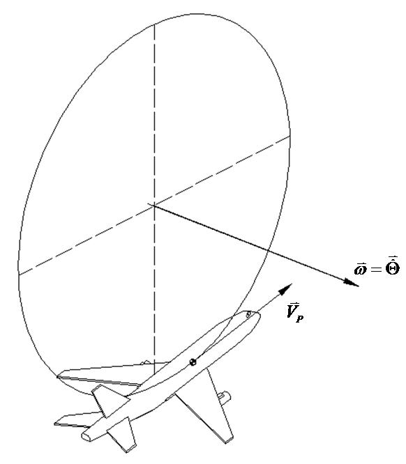
Figure P1.1.1 - Constant pitching maneuver

Using the steady state conditions,

A constant pitching maneuver implies:

With the above conditions, the GEs lead to:

and the KEs lead to:

Which

Finally, the CLMEs for this case are,

Constant Rolling Around the X-Axis

Figure P1.2 shows a constant rolling around the X-axis maneuver.

Figure P1.1.2 - Constant rolling around the X-axis

Using the steady state conditions:

a constant rolling around the X-axis implies:

Using the above conditions the KEs lead to:

In this case the CLMEs are given by:

Steady-Turning at Constant Altitude

Figure P1.3 shows a steady-turning at constant altitude maneuver.

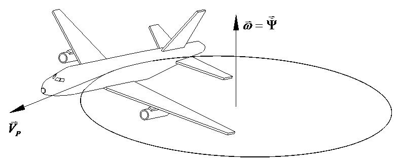
Figure P1.1.3 - Steady-turning at constant altitude

Using the steady state conditions:

A steady-turning at constant altitude implies:

Using the IKEs and the above conditions we obtain: sinsin coscossincossin coscossincoscos

Thus, the CLMEs for this case are:

Problem 1.2

Consider a Vertical Take Off Landing (VTOL) aircraft – such as the AV8 Harrier aircraft. Assume that the aircraft has a jet engine with a constant angular momentum RRhI

. Derive expressions for ,, XYZ hhh at the following configurations:

- rotor axis at angle of 90 deg tilted upwards with respect to the X axis;

- rotor axis at angle of 60 deg tilted upwards with respect to the X axis;

- rotor axis at angle of 30 deg tilted upwards with respect to the X axis;

- rotor axis aligned with the X axis.

Solution of Problem 1.2

The aircraft features one engine (N=1); therefore:

Case #1: rotor axis at angle of 90 deg tilted upwards with respect to the X-axis

In this case the engine angular momentum is along the aircraft Z-axis, then:

Case #2: rotor axis at angle of 60 deg tilted upwards with respect to the X-axis

Figure P2.1 shows this setting. It can be seen that:

Airplanebodyaxis

Rotoraxis

Figure P1.2.1 - Rotor tilted at 60 deg

Case 3: rotor axis at angle of 30 deg tilted upwards with respect to the X-axis

Figure P2.2 shows this setting. It can be seen that:

Airplanebodyaxis Rotoraxis

Figure P1.2.2 - Rotor tilted at 30 deg

Case 4: rotor axis aligned with the X-axis

In this case the engine angular momentum is along the aircraft X-axis; therefore:

Problem 1.3

Consider a Vertical Take Off Landing (VTOL) aircraft with a thrust vectoring system.

Assume that the aircraft has a jet engine with a constant angular momentum RRhI   .

Derive expressions for ,, XYZ hhh at the following configuration: - rotor axis at angle of 30 deg tilted upwards with respect to the X axis and at an angle of 20 deg. tilted to the right with respect to the X axis.

Solution of Problem 1.3

The aircraft features one engine (N=1); therefore:

Figure P3.1 shows the rotor angular momentum and its components. From the top triangle we have:

From the triangle at the bottom of the figure we have:

The magnitude of the angular momentum is given by,

Equating the expressions for Xh obtained from each triangle,

Therefore:

0.9210.9210.9540.879

Finally, using the expressions obtained from the above triangles:

Figure P1.3.1 - Rotor angular momentum

Problem 1.4

Demonstrate that the relationship between the components of the aircraft velocity in the body axes and the earth inertial frame (also known as Flight Path Equations), is given by:

' ' ' coscossincoscossinsinsinsincossincos sincoscoscossinsinsinsincossinsincos sincossincoscos

XU YV ZZ

Solution of Problem 1.4

Starting from:

XU YV ZZ

Define the following:

cossin0 sincos0 001 A

Therefore, we have:

Performing the first multiplication we have: cossin0cos0sincoscossincossin sincos0010sincoscossinsin 001sin0cossin0cos AB         leading to:



ABC

     

 coscossincossin100 sincoscossinsin0cossin sin0cos0sincos coscossincoscossinsinsinsincossincos sincoscoscossinsinsincossinsinsincos

  sincossincoscos       

Then, ' ' ' coscossincoscossinsinsinsincossincos sincoscoscossinsinsinsincossinsincos sincossincoscos

 

XU YV ZZ

  

Problem 1.5

Consider the „general‟ expression of the Conservation of Linear Momentum Equations (CLMEs) with respect to the body axes ,, XYZ

Demonstrate step-by-step how the introduction of the steady state and perturbed flight conditions, along with the introduction of the small perturbation assumptions leads to the

following „small perturbations‟ expression for the CLMEs with respect to the body axes ,, XYZ .

Specifically, explain why and how different terms out cancel out leading to the expressions above.

Solution of Problem 1.5

Using the definitions of steady state and perturbed flight:

By definition, at steady state conditions we

Inserting the above

  

  

Performing the multiplications in the left hand side:

11 11 11 111111111 1111111111 1111111111 sin cossin coscos XXXX YYYY ZZZ AATT AATT AAT muQWwQqWqwRVvRrVrvmgFfFf mvURrUuRurPWwPpWpwmgFfFf mwPVvPpVpvQUuQqUqumgFfF  

 

Using the following identities:   11111 sinsincoscossinsincos     11111 coscoscossinsincossin     11111 sinsincoscossinsincos     11111 coscoscossinsincossin  

The terms that contain „sin‟ and „cos‟ functions can be rewritten as:

 111111 11111111 cossincossinsincos cossincoscossinsinsincos

 

 

coscoscossincossin coscoscossinsincossinsin

 111111 11111111

   

Inserting in the CLMEs equations:





The first term in left hand side is equal to the two first terms in the right hand side in each equation, since they represent the steady state CLMEs. Therfore:



Next, using the small perturbation assumption: 0,0,0,0,0,0,0qwrvurpwpvqu

Therefore:





Finally, rearranging, we will have the FINAL “small perturbation” CLMEs:





YY ZZ AT AT AT muQwqWRvrVmgff mvUruRPwpWmgmgff mwPvpVQuUqmgmgff

cossinsincos



Problem 1.6

Consider the „general‟ expression of the Conservation of Angular Momentum Equations (CAMEs) with respect to the body axes ,, XYZ .

Demonstrate step-by-step how the introduction of the steady state and perturbed flight conditions, along with the introduction of the small perturbation assumptions leads to the following „small perturbations‟ expression for the CAMEs with respect to the body axes ,, XYZ .

Specifically, explain why and how different terms out cancel out leading to the expressions above.

Solution of Problem 1.6

Using the definitions of steady state and perturbed flight: 1 PPp  , 1 QQq

By definition of steady state conditions:

Inserting the above expressions in the

Performing the multiplications in the left hand side leads to:

pIrIPQqPpQpqIRQqRrQrqII LlLl

qIPRrPpRprIIPpPpRrRrI MmMm

rIpIPQqPpQpqIIQRrQqRqrI Nn 

ZZXZYYXXXZ AA

 1 TTNn 

Rearranging the above equations we have:

The first two terms in left hand side are equal to the two first terms in the right hand side in each equation, since they represent the steady state CAMEs, then

rIpIqPpQpqIIrQqRqrInn 

Next, using the small perturbation assumption, we have: 22 0,0,0,0,0pqrqprpr

Therefore:

YYXXZZXZAT ZZXZYYXXXZAT pIrIqPpQIqRrQIIll qIrPpRIIpPrRImm rIpIqPpQIIrQqRInn  

Finally, rearranging, we will have the FINAL „small perturbation‟ CAMEs:

Problem 1.7

Consider the Inverted Kinematic Equations (IKEs) under the assumption of small perturbations:

Explain under which conditions the above equations can be reduced to the following expressions:

Solution of Problem 1.7

Assuming initial steady state flight conditions we have:

Thus, the given equations become:

Next, assuming initial wing level flight ( 1 0

) the above equations become:

Finally, assuming no initial pitch angle 1 (0)

, we have:

Thus the required conditions are:

 Initial steady state flight

 Initial wing level flight ( 1 0  )

 No initial pitch angle 1 (0) 

Problem 1.8

Consider the drawings below with the dimensions of 4 „extra large‟ aircraft.

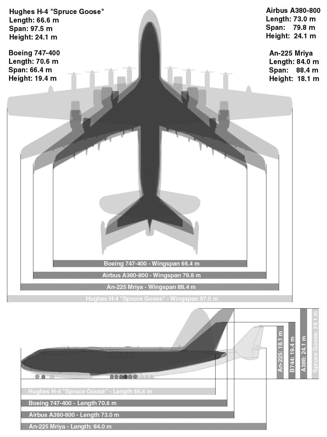
Figure P1.8.1 –

(Source: http://upload.wikimedia.org/wikipedia/commons/9/96/Giant_Plane_Comparison.jpg)

Using your best technical judgment, rank the values of all the moments of inertia for the different aircraft. Document your response with simple calculations using approximate distances.

Solution of Problem 1.8

The moment of inertia XX I which represents the inertial resistance of the aircraft to a change in its angular velocity around the X- axis (rolling velocity). Clearly, it is more difficult to change the rolling velocity of an aircraft with a larger wingspan; the presence of engines in the wing can only increase this inertia, since they add mass to the wing. According to this and assuming that the engines of all the aircrafts have approximately the same weight (the H4 engines are smaller but they are piston engines while the other three aircraft have turbofan engines) the XX I can be ranked according to Table P1.8.1.

Similarly, the moment of inertia YYI represents the inertial resistance of the aircraft to a change in its angular velocity around the Y- axis (pitching velocity), which is located at the aircraft CG. The CG is located at approximately 25% of the mean aerodynamic chord; even without this information, it can be stated that the CG is located at a stating approximately on the wing. Therefore, the weight distributed in the fuselage – not in the wings - is the main provider to this moment of inertia. Therefore, the value for this parameter can be ranked according to the fuselage length; this, the longer the fuselage the larger the value of YYI . The results are presented in Table P1.8.1.

Similarly, the moment of inertia ZZI represents the inertial resistance of the aircraft to a change in its angular velocity around the Z- axis (yawing velocity), which is located at the aircraft CG In this case, the contribution of the masses located in both the fuselage and wings are important. The Antonov‟s wings and fuselage are larger than the Airbus‟; the Airbus‟ wings and fuselage are larger than the Boeing‟s; therefore, it can be stated that their ZZI are in the same order of magnitude. For this case it is difficult to say if

Hughes‟ ZZI is greater than Antonov‟s since, although the Hughes H-4 has a larger wingspan, it is a lighter aircraft (made of wood) and has a smaller fuselage; therefore, a more detailed knowledge of the structural density and mass distribution is required for an accurate analysis.

A comprehensive ranking is provided below (with some approximation for ZZI )

Aircraft

Problem 1.9

( XX I )

Table P1.8.1 – Ranking of the Moments of Inertia

Consider the F111 aircraft shown in the drawing below.

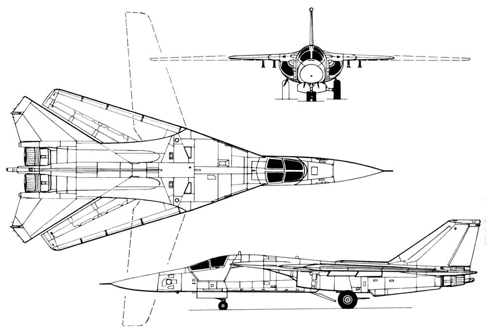
Figure P1.9.1 - 3D View of the General Dynamic F-111 Aircraft (Source: http://www.aviastar.org/index2.html)

I )

Using your best technical judgment, explain how the values of all the moments of inertia change when the configuration of the aircraft is changed from the low-subsonic forward wing position (low sweep angle) to the high-subsonic high-sweep angle position.

Solution of Problem 1.9

The moment of inertia XX I which represents the inertial resistance of the aircraft to a change in its angular velocity around the X- axis (rolling velocity) XX I will decrease as the wing sweep angle increases, since it is more difficult to change this velocity of an aircraft with a larger wingspan ( the mass distribution is now closer to the axis of rotation). A similar trend is expected for ZZI . The opposite trend is expected for the

moment of inertia YYI . This is due to the fact that the masses in the wing will shift further down toward the tail with respect to the aircraft CG. Therefore, YYI will increase as the wing sweep angle increases. Table P9.1 summarizes the trends.

Moment of inertia

FROM low wing sweep angle (subsonic) TO high wing sweep angle (supersonic)

Problem 1.10

Decreases Increases Decreases

Table P1.9.1 – Trends for moments of inertia

Consider the Lockheed L-1011 “Tristar” aircraft shown in the drawing below.

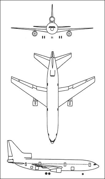
Figure P1.10.1 - 3D View of the Lockheed L-1011 Aircraft (Source: http://www.aviastar.org/index2.html)

Assuming that at steady state conditions the throttle setting is the same for each of the 3 aircraft engines, first introduce generic distances along the body axes ,, XYZ of the distances of each of the engines with respect to the aircraft center of gravity. Next, qualitatively describe how the terms ,,,,,XYZ TTTTTT FFFLMN in the CLMEs and CAMEs are modified under the following engine failure conditions: - failure of the tail engine; - failure of the wing engine on the right of the pilot.

Assume that in both cases the failures occur while the aircraft is in steady-state rectilinear flight conditions.

Solution of Problem 1.10

At steady-state rectilinear flight conditions:

Figure P1.10.2 shows the distances of each of the engines from the aircraft center of gravity

Figure P1.10.2 - Distances of the engines with respect to the aircraft center of gravity

Assume:

This means that each of the engines generates the same thrust , EF , and only in the X direction. Additionally:

Condition 1. Failure of the tail engine In this case, the above force/moments equations will become: 1

Condition 2. Failure of the wing engine on the right of the pilot. In this case, the above force/moments equations will become:

Problem 2.1

Problems for Chapter II

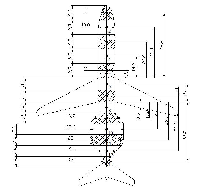
Consider the data relative to the Aeritalia G91 aircraft in Appendix C. Use the provided drawings to extract all the relevant geometric characteristics of the aircraft. Provide estimates for the following parameters:

Solution of Problem 2.1

All the relevant geometric parameters were extracted from the images in Appendix C, as shown below.

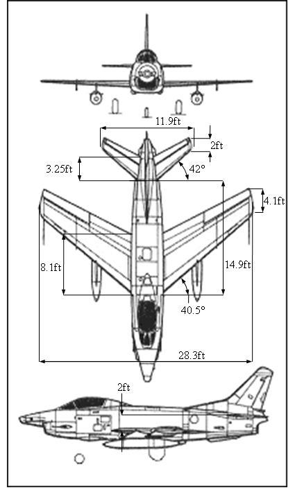
Figure P2.1.1 - MODIFIED 3D View of Aeritalia Fiat G91 Aircraft (Source: http://www.aviastar.org/index2.html)

Specifically, the following geometric parameters were identified: 4.1,8.1,40.50.707, 14.9,2 R TRLEWHWH cftcftradXftZft

Next, using the assumption of straight wings, the following additional wing and tail geometric parameters were derived using the above values:

Wing Geometric Parameters

0.50.5 40.5(1)40.5(10.506) tantantan(0.707)0.617 (1)4.525(10.506) LE rad AR

0.250.25 40.25(1)40.25(10.506) tantantan(0.707)0.663 (1)4.525(10.506) LE rad AR

22 2(1)2(10.6150.615)3.252.675 3(1)3(10.615)

(12)11.9(120.615)tan()tan(0.722)2.466 6(1)6(10.615)

Wing-Tail Geometric Parameters

The following sketch was derived to illustrate the wing-tail geometric distances.

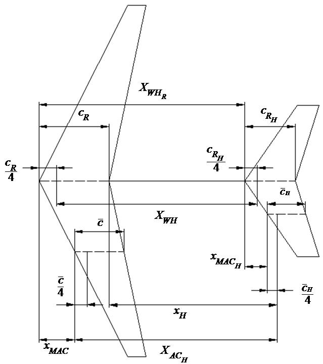
Figure P2.1.2-Wing-Horizontal Tail Geometric Distances

From the above figure:

Knowing that 14.9 R

Also, knowing that 2 WH Zft  , the wing-tail geometric parameters needed for the analysis of the downwash effect are given by:

Recall that the meaning of the geometric parameters ‘m’ and ‘r’ – shown in Figure P2.1.3 below - was introduced in the analysis of the downwash effect (Section 2.4)

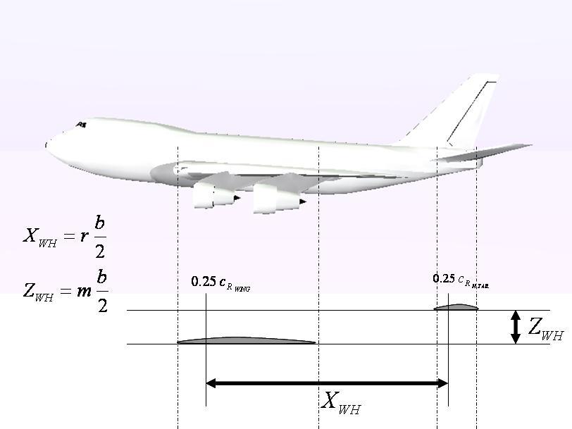
Figure P2.1.3-Geometric Parameters for the Downwash Effect

From Figure P2.1.2 the parameter HACx can be found using:

Note that LE is outside the valid range for the Polhamus formula. Therefore, the above estimate is somewhat approximate and in excess of its true value.

Modeling of

Wing Aerodynamic Center

This parameter can be obtained using the following relationship,

shere

The following parameters are required in Figure 2.27:

Interpolating between the curves of the plots of Figures 2.25 using 0.506  and tan3.86

we have: 0.869

From interpolation of Figure 2.28, using 1 0.5061.282 K 

From interpolation of Figure 2.29, using

Therefore, the location of the wing aerodynamic center is estimated at:

The aerodynamic center shift due to the body is calculated using the so-called Munk theory (Section 2.5):

ibw , ix are geometric parameters for discretized aircraft sections, as shown below.

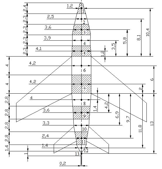
P2.1.4 - Aircraft sections for calculations of WBACx (Dimensions in ft)

The parameter i d d  

is calculated through the 2 curves in Figure P1.5 below.

Figure

Figure P2.1.5 - Downwash Calculations for WBACx

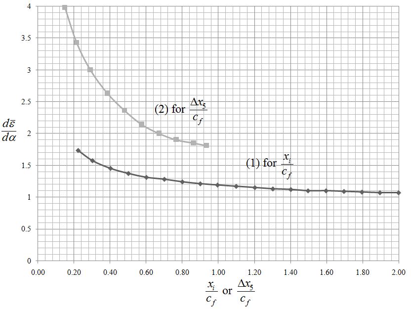
Specifically,

for 1,2,3,4,5 i  is obtained using curve (1) using the required

values for ix with 8.1 fRoot ccft  .For 5 i  ,

is obtained using curve (2) and

taking into account that 5 2.3 xft . Finally, for 6...13 i  ,

The value of

From Figure P2.1.2:

and the final results are summarized in Table P2.1.1 below.

Table P2.1.1 – Calculations for WBACx

Problem 2.2

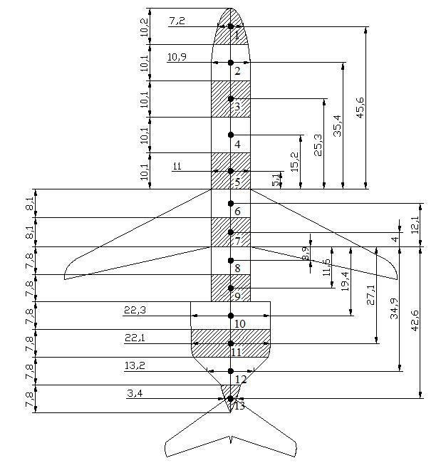
Consider the data relative to the Beech 99 aircraft in Appendix B and Appendix C. Use the provided drawings to extract all the relevant geometric characteristics of the aircraft. Provide estimates for the following parameters:

Solution of Problem 2.2

All the relevant geometric parameters were extracted from the images in Appendix C, as shown below.

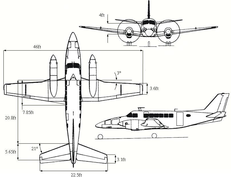
Figure P2.2.1 - MODIFIED 3D View of Beech 99Aircraft (Source: http://www.aviastar.org/index2.html)

Specifically, the following geometric parameters were identified:

3.6,7.85,30.052, 20.8,4 R TRLEWHWH cftcftradXftZft  22.5,3.1,5.65,210.367 HHH HTRLE bftcftcftrad 

Next, using the assumption of straight wings, the following additional wing and tail geometric parameters were derived using the above values:

Wing Geometric Parameters

3.6

Wing-Tail Geometric Parameters

The sketch in Figure P2.2.2 was derived to illustrate the wing-tail geometric distances.

Figure P2.2.2-Wing-Horizontal Tail Geometric Distances

From Figure P2.2.2:

Also, knowing that 4 WH Zft  , the wing-tail geometric parameters needed for the analysis of the downwash effect are given by:

Recall that the meaning of the geometric parameters ‘m’ and ‘ r’ – shown in Figure P2.3 below - was introduced in the analysis of the downwash effect (Section 2.4)

P2.2.3-Geometric Parameters for the Downwash Effect

From Figure P2 2.2 the coordinate HACx can be found using:

Figure

Wing Lift-Slope Coefficient

An important limitation of the application of the Polhamus formula should be pointed out. The above relationship does not model the disturbing effect of the engines and the engine nacelles under the wing. Therefore, the above value for the wing-lift curve slope should be considered to be somewhat higher than the actual value.

Horizontal Tail Lift Slope Coefficient

Modeling of the Downwash Effect

Wing Aerodynamic Center

This parameter

The

Interpolating the between the curves of the plots of Figures 2.25 using 0.459

and

tan0.396 LE AR  we have: 0.242 AC R x c  

From interpolation of Figure 2.26, using 1 0.4591.31 K 

From interpolation of Figure 2.27, using 3 LE  , 0.459  , 2 7.5570.069ARK

Therfore, the location of the wing aerodynamic center is estimated at:

Modeling of WBACx

The aerodynamic center shift due to the body is calculated using the so-called Munk theory (Section 2.5):

ibw , ix are geometric parameters for discretized aircraft sections, as shown below.

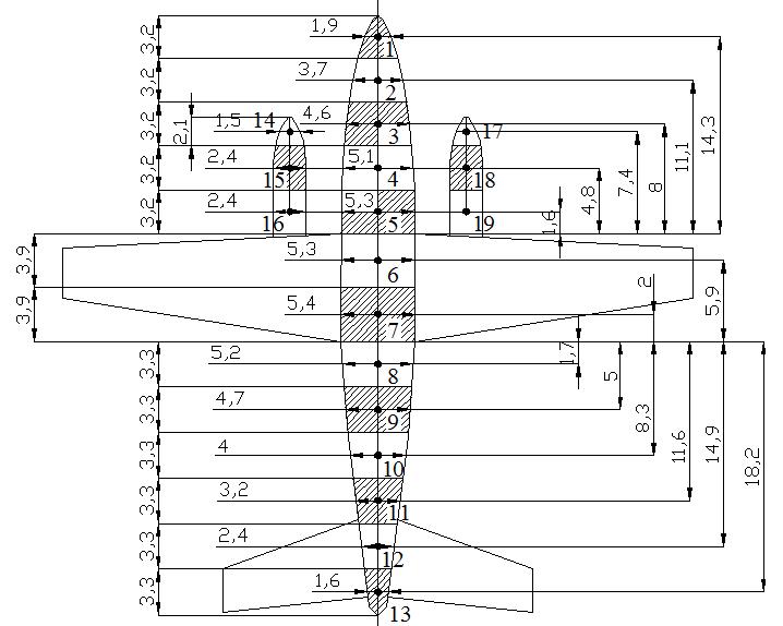
Figure P2.2.4 - Aircraft sections for calculations of WBACx (Dimensions in ft)

The parameter i d d  

is calculated through the 2 curves in Figure P2.5 below.

P2.2.5 - Downwash Calculations for WBACx

Figure

Specifically,

for 1,2,3,4,5 i  is obtained using curve (1) using the required

values for ix with 7.85 fRoot ccft  .For 5 i  ,

is obtained using curve (2) and

taking into account that 5 3.2 xft . Finally, for 6...13 i  ,

The value of

Figure P2.2:

The values for

and the final results are summarized in Table P2.1 below. Note that the effect of the nacelles – which is significant for this aircraft - is also included.

Problem 2.3

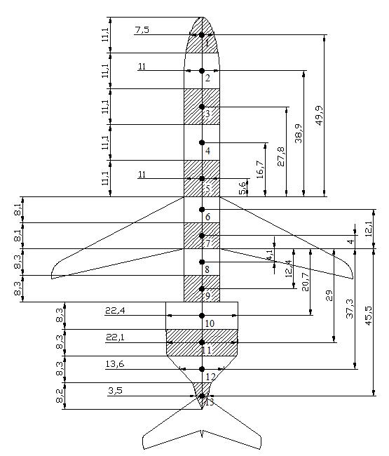
Consider the data relative to the Cessna T37 aircraft in Appendix B and Appendix C. Use the provided drawings to extract all the relevant geometric characteristics of the aircraft. Provide estimates for the following parameters:

Solution of Problem 2.3

All the relevant geometric parameters were extracted from the images in Appendix C, as shown below.

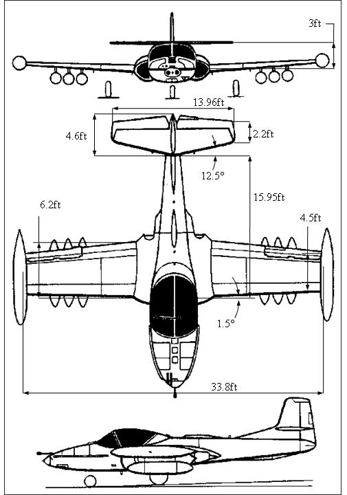
Figure P2.3.1 - MODIFIED 3D View of Cessna T37 Aircraft (Source: http://www.aviastar.org/index2.html)

Specifically, the following geometric parameters were identified:

4.5,6.2,1.50.026, 15.95,3 R TRLEWHWH cftcftradXftZft  13.96,2.2,4.6,12.50.218 HHH HTRLE bftcftcftrad 

Next, using the assumption of straight wings, the following additional wing and tail geometric parameters were derived using the above values:

Wing Geometric Parameters

4.5

0.50.5

0.50.5 40.5(1)40.5(10.478) tantantan(0.218)0.050 (1)4.106(10.478)

Wing-Tail Geometric Parameters

The sketch in Figure P2.3.2 was derived to illustrate the wing-tail geometric distances.

Figure P2.3.2-Wing-Horizontal Tail Geometric Distances

From Figure P2.3.2:

Knowing that 15.95 RWH Xft  :

Also, knowing that 3 WH Zft  , the wing-tail geometric parameters needed for the analysis of the downwash effect are given by:

Recall that the meaning of the geometric parameters ‘m’ and ‘r’ – shown in Figure P3.3. below - was introduced in the analysis of the downwash effect (Section 2.4)

Figure P2.3.3-Geometric Parameters for the Downwash Effect

From Figure P2.3.2 the coordinate HACx can be found using:

Solving for H

Wing Lift-Slope Coefficient

Horizontal Tail Lift Slope Coefficient

Modeling of the Downwash Effect

Wing Aerodynamic Center

This

Interpolating between the curves of the plots of Figures 2.25, using 0.726  and

tan0.164 LE AR  we have: 0.248

From interpolation of Figure 2.28, using 1 0.7261.143 K 

From interpolation of Figure 2.29, using

Therefore, the location of the wing aerodynamic center is estimated at:

Modeling of

The aerodynamic center shift due to the body is calculated using the so-called Munk theory (Section 2.5):

ibw , ix are geometric parameters for discretized aircraft sections, as shown below.

Figure P2.3.4 - Aircraft sections for calculations of WBACx (Dimensions in ft)

The parameter i d d  

is calculated through the 2 curves in Figure P2.3.5 below.

Figure P2.3.5 - Downwash Calculations for WBACx

Specifically,

for 1,2,3,4,5 i  is obtained using curve (1) using the required

values for ix with 6.2 fRoot ccft  .For 5 i  ,

taking into account that

The value of

is obtained using curve (2) and

From Figure P3.2 we

The

and the final results are summarized in the table below.

Table P2.3.1 – Calculations for WBACx

Problem 2.4

Consider the data relative to the McDonnell Douglas DC-9 aircraft in Appendix C. Next, consider the later versions of the DC-9 aircraft which were introduced later in its operational life.

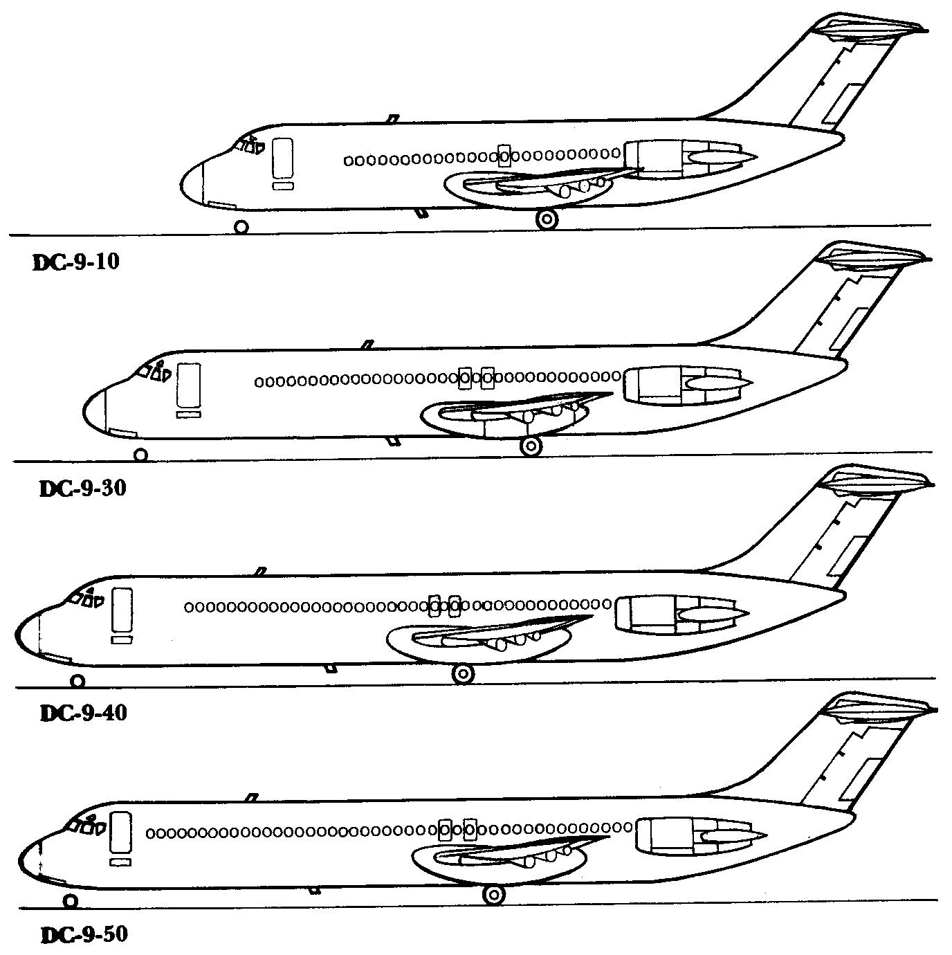
Figure P2.4.1 - Lateral Views McDonnell Douglas DC 9 Series 10/30/40/50 (Source: http://www.aviastar.org/index2.html)

Ref. [30] provides detailed information about the differences in the geometric parameters.

The geometric parameters for the DC 9 Series 10/30/40/50 aircraft are summarized in the tables below.

Wing Geometric Parameters (as shown in Student Sample Problem #1)

Table P2.4.1 – Wing Geometric Parameters

Horizontal Tail Geometric Parameters (as shown in Student Sample Problem #1)

Table P2.4.2 – Horizontal Tail Geometric Parameters

Wing-Tail Geometric Parameters (as shown in Student Sample Problem #1)

Figure P2.4.2 - Wing-Horizontal Tail Geometric Distances

Table P2.4.3 – Wing Geometric Parameters

Using the above geometric information derived from Ref.[30], provide estimates for the following parameters for the DC-9 30, DC-9 40, and DC-9 50:

Solution of Problem 2.4

Using the geometric parameters provided in Tables P4.1, P4.2, and P4.3, the following tables summarize the results for the different versions of the DC-9 aircraft using the same procedure outlined in Student Sample Problem #1 (SSP#1). The data for the Series 10 aircraft previously calculated in SSP #1 are here provided for a benchmark comparison.

Wing Lift-Slope Coefficient for Different DC-9 Versions

Table P2.4.4 – Wing Lift-Slope Coefficient

Modeling of the Downwash Effect for Different DC-9 Versions

Table P2.4.5 –Downwash effect

Wing

Aerodynamic Center for Different DC-9 Versions

Table P2.4.6 – Wing Aerodynamic Center

Modeling of WBACx

Once again, the aerodynamic center shift due to the body is calculated using the so-called Munk theory (Section 2.5). Figures P4.3, P4.4, and P4.5 show the sections of the different aircraft for the calculations of WBACx . These figures were drawn using the geometric values derived from the images in Ref.[30].

Figure P2.4.3 - Aircraft sections for calculations of WBACx (Dimensions in ft). DC9-30 Aircraft

P2.4.4

Figure

- Aircraft sections for calculations of WBACx (Dimensions in ft). DC9-40 Aircraft

P2.4.5 - Aircraft sections for calculations of WBACx (Dimensions in ft). DC9-50 Aircraft

Figure

Table P2.4.7 – Calculations for WBACx . DC9-30 Aircraft

Table P2.4.8 – Calculations for WBACx . DC9-40 Aircraft

Problem 2.5

Consider the data relative to the McDonnell Douglas F-4 aircraft in Appendix C. Use the provided drawings to extract all the relevant geometric characteristics of the aircraft. Provide estimates for the following parameters:

Solution of Problem 2.5

From the drawings in Appendix C, the following geometric parameters were identified: 38.7,4.7,18,48.50.846, 28,4 R TRLEWHWH bcftcftradXftZft  16.4,2.2,7.6,430.75 HHH HTRLE bftcftcftrad 

Next, using the assumption of straight wings, the following additional wing and tail geometric parameters were derived using the above values:

Wing Geometric Parameters 4.7 0.261

0.250.25 40.25(1)40.25(10.261) tantantan(0.846)0.745 (1)2.826(10.261) LE rad AR

Wing-Tail Geometric Parameters

The following sketch was derived to illustrate the wing-tail geometric distances.

Figure P2.5.1 - Wing-Horizontal Tail Geometric Distances

From the above figure:

Knowing that 28 R

Also, knowing that 4 WH Zft  , the wing-tail geometric parameters needed for the analysis of the downwash effect are given by:

Recall that the meaning of the geometric parameters ‘m’ and ‘r’ – shown in Figure P2.5.2 below - was introduced in the analysis of the downwash effect (Section 2.4)

Figure P2.5.2-Geometric Parameters for the Downwash Effect

From Figure P2.5 1 the parameter HACx can be found using:

Wing Lift-Slope Coefficient

Note that LE , AR and  are outside the valid range for the Polhamus formula.

Therefore, the above estimate is to be considered somewhat approximated.

Modeling of the Downwash Effect

Wing Aerodynamic Center

This parameter can be obtained using the following relationship,

shere AC R x c

, 1K and 2K are obtained from Figures 2.27, 2.28, and 2.29 respectively.

The following parameters are required in Figure 2.27:

Interpolating between the curves of the plots of Figures 2.25 using 0.261  and tan3.194

From interpolation of Figure 2.28, using 1 0.2611.42

From interpolation of Figure 2.29, using

Therefore, the location of the wing aerodynamic center is estimated at:

Modeling of

The aerodynamic center shift due to the body is calculated using the so-called Munk theory (Section 2.5):

ibw , ix are geometric parameters for discretized aircraft sections, as shown below.

Figure P2.5.3 - Aircraft sections for calculations of WBACx (Dimensions in ft)

The parameter

is calculated through the 2 curves in Figure P2.5.4 below.

Figure P2.5.4 - Downwash Calculations for WBACx

Specifically, i d d

for 1,2,3,4,5 i  is obtained using curve (1) using the required values for ix with 18 fRoot ccft  .For 5 i  , i

is obtained using curve (2) and taking into account that 5 4.5 xft . Finally, for 6...13 i  ,

The

is the downwash effect evaluated with 0 m  , thus:

From Figure P2.5.1:

The values for

and the final results are summarized in Table P2.5.1 below.

Table P2.5.1 – Calculations for WBACx

Problem 2.6

Consider the data relative to the McDonnell Douglas DC-8 aircraft in Appendix C. Use the provided drawings to extract all the relevant geometric characteristics of the aircraft. Provide estimates for the following parameters:

Solution of Problem 2.6

From the drawings in Appendix C, the following geometric parameters were identified: 142.5,7.9,31.5,340.593, 80.9,7.3 R TRLEWHWH bcftcftradXftZft  47.9,6.4,14.4,390.681 HHH HTRLE bftcftcftrad

Next, using the assumption of straight wings, the following additional wing and tail geometric parameters were derived using the above values:

Wing Geometric Parameters

Wing-Tail Geometric Parameters

The following sketch was derived to illustrate the wing-tail geometric distances.

Figure P2.6.1-Wing-Horizontal Tail Geometric Distances

From the above figure:

Knowing that 28 R

Also, knowing that 7.3 WH Zft  , the wing-tail geometric parameters needed for the analysis of the downwash effect are given by:

Recall that the meaning of the geometric parameters ‘m’ and ‘r’ – shown in Figure P2.6.2 below - was introduced in the analysis of the downwash effect (Section 2.4)

Figure P2.6.2-Geometric Parameters for the Downwash Effect

From Figure P2.6 1 the parameter HACx can be found using:

Wing Lift-Slope Coefficient

Modeling of the Downwash Effect

Wing Aerodynamic Center

This

shere AC R x c  , 1K and 2K are obtained from Figures 2.27, 2.28, and 2.29 respectively.

The following parameters are required in Figure 2.27:

Interpolating between the curves of the plots of Figures 2.25 using 0.251  and tan4.939 LE

From interpolation of Figure 2.28, using 1 0.2511.425 K

From interpolation of Figure 2.29, using

Therefore, the location of the wing aerodynamic center is estimated at:

The aerodynamic center shift due to the body is calculated using the so-called Munk theory (Section 2.5):

ibw , ix are geometric parameters for discretized aircraft sections, as shown below.

Figure P2.6.3 - Aircraft sections for calculations of WBACx (Dimensions in ft)

The parameter

is calculated through the 2 curves in Figure P2.6.4 below.

Figure P2.6.4 - Downwash Calculations for WBACx

Specifically, i

for 1,2,3,4,5 i  is obtained using curve (1) using the required values for ix with 31.5 fRoot ccft  .For 5 i  , i

is obtained using curve (2) and taking into account that 5 9.6 xft . Finally, for 6...13 i  ,

The value of

is the downwash effect evaluated with 0 m  , thus:

From Figure P2.6.1:

Therefore:

The values for

and the final results are summarized in Table P2.6.1 below. Note that the effect of the nacelles – which is significant for this aircraft - is also included.

Table P2.6.1 – Calculations for WBACx

Problems for Chapter III

Problem 3.1

Consider the data relative to the Aeritalia G91 aircraft in Appendix C. Use the provided drawings to extract all the relevant geometric characteristics of the aircraft. Assume that this aircraft features both stabilators and elevators for the control of the longitudinal dynamics. Also assume 0.38,0.88EH  . Using the modeling outlined in this chapter, find a numerical value for the following aerodynamic parameters:

Solution of Problem 3.1

All the relevant geometric parameters were extracted from the provided images in Appendix C. Specifically, the following geometric parameters were identified:

4.1,8.1,40.50.707, 14.9,2 R TRLEWHWH cftcftradXftZft  11.9,2,3.25,420.733

Next, using the assumption of straight wings, the following wing and tail geometric parameters were derived using the above values:

Horizontal Tail Geometric Parameters

Wing-Tail Geometric Parameters From Problem 2.1

Note that HLE is outside the valid range for the Polhamus formula. Therefore, the above estimate is somewhat approximate (in excess of its true value).

Modeling of the Downwash Effect

From Problem 2.1:

It should be emphasized that the above estimates are affected by the approximation associated with the previous estimates using Polhamus formula. Finally, the aircraft aerodynamic center can be determined using:

3.83531.238 0.1970.8810.4952.002 3.952177 0.325 3.83531.238 10.8810.495 3.952177

The above value is consistent with typical ACx values for this class of aircraft.

Problem 3.2

Consider again the Aeritalia G91 aircraft in Appendix C. Use the provided drawings to extract all the relevant geometric characteristics of the aircraft. Assume 0.88 H  Using the modeling outlined in this chapter, find a numerical value for the following aerodynamic parameters:

Solution of Problem 3.2

Wing Parameters

From Problems 2.1 and 3.1:

Parameters

Downwash Effect From

Stability Derivatives

The following derivatives are calculated using the modeling shown in Section 3.9.3.

Problem 3.3

Assume 0.45,0.85EH  Using the modeling outlined in this chapter, find a numerical value for the following aerodynamic parameters:

Next, compare the obtained values with the TRUE values listed in Appendix B (Aircraft #3) and evaluate the error associated with the use of the ‘empirical’ modeling approach.

Solution of Problem 3.3

All the relevant geometric parameters were extracted from the provided images in Appendix C. Specifically, the following geometric parameters were identified: 3.6,7.85,30.052, 20.8,4 R TRLEWHWH cftcftradXftZft

22.5,3.1,5.65,210.367

Next, using the assumption of straight wings, the following wing and tail geometric parameters were derived using the above values:

Horizontal Tail Geometric Parameters

tantantan(0.367)0.264 (1)5.143(10.549)

Wing-Tail Geometric Parameters

From Problem 2.2: 3.592

Wing Lift-Slope Coefficient

From Problem 2.2: 5.249

Horizontal Tail Lift Slope Coefficient

Modeling

Comparison between TRUE Values and ‘Empirical’ Values

A comparison between the true values of the above derivatives and their estimates using the ‘empirical’ aerodynamic modeling approach, along with a calculation of the percentage of the error, is shown in the Table below:

BEECH 99

Table P3.3.1 – Comparison between ‘Empirical’ and True Values

The analysis of the results in the above table reveals the following:

- The substantial error in the value of Lc  is likely due to the fact that the empirical approach overestimates this coefficient since it does not properly model the loss of lift due to the large engine nacelles on the wings.

- The substantial error in the value of mc  is likely due to 2 distinct sources.

, the overestimate of mc  is due to the overestimate of Lc  . Additionally, it is due to the previous overestimate of 0.580

x  , which was again based on the overestimate of Lc  . From the ‘true values’ for ,

, we would have:

Problem 3.4

Consider again the data relative to the Beech 99 aircraft in Appendix B and Appendix C. Use the provided drawings to extract all the relevant geometric characteristics of the aircraft. Assume 0.85 H  . Using the modeling outlined in this Chapter, find a numerical value for the following aerodynamic parameters:

Next, compare the obtained values with the TRUE values listed in Appendix B (Aircraft #3) and evaluate the error associated with the use of the ‘empirical’ modeling approach.

Solution of Problem 3.4

Wing Parameters

Again, from Problem 2.2:

Horizontal Tail Parameters From Problems 2.2 and Problem 3.3:

From Problem 2.2:

Stability Derivatives

The following derivatives are calculated using the modeling presented in Section 3.9.3,

Calculating

Given the large aspect ratio of the wing ( 7.557 AR  ), we have:

Comparison between TRUE Values and ‘Empirical’ Values

BEECH 99

Table P3.4.1 – Comparison between ‘Empirical’ and True Values

The errors in the values of Lc  and mc  are typical for the empirical estimates for these derivatives.

Problem 3.5

Assume 0.43,0.9EH  . Using the modeling outlined in this chapter, find a numerical value for the following aerodynamic parameters:

Next, compare the obtained values with the TRUE values listed in Appendix B (Aircraft #4) and evaluate the error associated with the use of the ‘empirical’ modeling approach.

Solution of Problem 3.5

All the relevant geometric parameters were extracted from the provided images in Appendix C. Specifically, the following geometric parameters were identified: 4.5,6.2,1.50.026, 15.95,3 R TRLEWHWH cftcftradXftZft  13.96,2.2,4.6,12.50.218

Next, using the assumption of straight wings, the following wing and tail geometric parameters were derived using the above values:

Horizontal Tail Geometric Parameters

Wing-Tail Geometric Parameters

From

Wing Lift-Slope Coefficient

Horizontal Tail Lift Slope Coefficient

Finally,

Comparison between TRUE Values and ‘Empirical’ Values

CESSNA T37

Empirical Values True Values Percent Error [%]

Table P3.5.1 – Comparison between ‘Empirical’ and True Value

It seems that the key stability and control derivatives are estimated with a desirable level of accuracy. Since

Problem 3.6

Consider again the data relative to the Cessna T37 aircraft in Appendix B and Appendix C. Use the provided drawings to extract all the relevant geometric characteristics of the aircraft. This aircraft features elevators for both trimming and maneuver purposes.

Assume 0.9 H  . Using the modeling outlined in this chapter, find a numerical value for the following aerodynamic parameters:

Next, compare the obtained values with the TRUE values listed in Appendix B (Aircraft #4) and evaluate the error associated with the use of the ‘empirical’ modeling approach.

Solution of Problem 3.6

Wing Parameters

From Problems 2.3 and 3.5:

Stability Derivatives

The following derivatives are calculated using the modeling presented in Section 3.9.3,

Comparison between TRUE Values and ‘Empirical’ Values

CESSNA T37

Table P3.6.1 – Comparison between ‘Empirical’ and True Value

The errors in the values of ,,, q q LLmm cccc   are typical for the empirical estimates for these derivatives with the most significant error reported on qLc

Problem 3.7

Consider the data relative to the McDonnell Douglas DC-9 Series 10 aircraft in Appendix C. Use the provided drawings to extract all the relevant geometric characteristics of the aircraft. This aircraft features stabilators for trimming and elevators for maneuver purposes. Assume 0.5 E  . Consider as ‘baseline’ the following numerical estimates of the longitudinal stability and control derivatives for the DC 9 Series 10 aircraft (see Student Sample Problem #1):

Next, consider the later versions of the DC-9 aircraft which were introduced later in its operational life.

Figure P3.7.1 - Lateral Views McDonnell Douglas DC 9 Series 10/30/40/50 (Source: http://www.aviastar.org/index2.html)

Ref. [9] provides detailed information about the differences in the geometric parameters. The geometric parameters for the DC 9 Series 10/30/40/50 aircraft are summarized in the tables below.

Wing Geometric Parameters (as shown in SSP#1-Chapter II)

Table P3.7.1 – Wing Geometric Parameters

Horizontal Tail Geometric Parameters (as shown in SSP #1- Chapter II)

Table P3.7.2 – Horizontal Tail Geometric Parameters

Wing-Tail Geometric Parameters (as shown in SSP #1, Chapter II)

Figure P3.7.2 - Wing-Horizontal Tail Geometric Distances

Table P3.7.3 – Wing Geometric Parameters

Using the above geometric information derived from Ref.[9], provide estimates for the following parameters for the DC-9 30, DC-9 40, and DC-9 50:

for the Mc Donnell Douglas DC 9 Series 30, 40, and 50. Also estimate the location of the aircraft aerodynamic center ACx for all the different versions of the aircraft.

Solution of Problem 3.7

Using the data provided in the above tables derived from Ref.[9], along with some of key results from Chapter II problems, we would have:

Wing Lift-Slope Coefficient

Table P3.7.4 – Wing Lift-Slope Coefficient

Horizontal Tail Lift Slope Coefficient

Table P3.7.5 – Horizontal Tail Lift-Slope Coefficient

Modeling of the Downwash Effect

From Problem 2.4:

Table P3.7.6 – Downwash effect

Modeling of WBACx

A relationship for WBACx is given by:

Next, using results from Problem 2.4:

Table P3.7.7 – Modeling of WBACx

Stability and Control Derivatives

Table P7.8 shows the empirical estimates of the values of the stability and control derivatives for the DC9-10/30/40/50 aircraft using the above calculated geometric parameters in the relationships:

Table P3.7.8 – Stability and Control Derivatives

Finally, the aircraft aerodynamic center can be determined using:

Results are presented in Table P7.9

Table P3.7.9 –Aircraft aerodynamic center

Problem 3.8

Consider again the data relative to the McDonnell Douglas DC-9 Series 10 aircraft in Appendix C. Use the provided drawings to extract all the relevant geometric characteristics of the aircraft. This aircraft features stabilators for trimming and elevators for maneuver purposes. Assume 0.5 E  . Consider as ‘baseline’ the following numerical estimates of the longitudinal stability and control derivatives for the DC 9 Series 10 aircraft (see Student Sample Problem #1):

Next, consider the later versions of the DC-9 aircraft which were introduced later in its operational life.

Figure P3.8.1 - Lateral Views McDonnell Douglas DC 9 Series 10/30/40/50 (Source: http://www.aviastar.org/index2.html)

Ref. [9] provides detailed information about the differences in the geometric parameters. The geometric parameters for the DC 9 Series 10/30/40/50 aircraft are summarized in the tables below.

Wing Geometric Parameters (as shown in SSP#1-Chapter II)

Table P3.8.1 – Wing Geometric Parameters

Horizontal Tail Geometric Parameters (as shown in SSP #1- Chapter II)

Table P3.8.2 – Horizontal Tail Geometric Parameters

Wing-Tail Geometric Parameters (as shown in SSP #1, Chapter II)

Figure P3.8.2 - Wing-Horizontal Tail Geometric Distances

Table P3.8.3 – Wing Geometric Parameters

Using the above geometric information derived from Ref.[9], provide estimates for the following parameters for the DC-9 30, DC-9 40, and DC-9 50: ,,, qq LLmm cccc

Solution of Problem 3.8

Summary of the Wing Geometric and Aerodynamic Parameters

From Problems 2.4 and 3.7:

Table P3.8.4 – Wing Parameters

Summary of the Horizontal Tail Geometric and Aerodynamic Parameters

From Problem 3.7:

Downwash Effect

From Problem 2.4:

Table P3.8.5 – Horizontal tail parameters

Table P3.8.6 – Downwash effect

Stability Derivatives

The following derivatives are calculated using the modeling presented in Section 3.9.3. The results are summarized in Table P3.8.7

Table P3.8.7 – Stability Derivatives

Problem 3.9

Consider the data relative to the Boeing B747 200 aircraft in Appendix B at high cruise conditions (Mach=0.9) and Appendix C. Use the provided drawings to extract all the relevant geometric characteristics of the aircraft. Assume that this aircraft features stabilators for trimming and elevators for maneuver purposes. Assume 0.47,0.85EH  . Using the modeling outlined in this chapter, find a numerical value for the following aerodynamic parameters:  ,,WWBACAC

 ,, i EH LLL ccc 

 ,,, i EH ACmmm xccc 

Next, compare the obtained values with the TRUE values listed in Appendix B (Aircraft #7) and evaluate the error associated with the use of the ‘empirical’ modeling approach.

Solution of Problem 3.9

All the relevant geometric parameters were extracted from Figure P3.9.1 below.

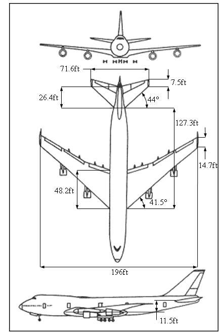
P3.9.1 - MODIFIED 3D View of Boeing 747-200Aircraft

Specifically, the following geometric parameters were identified: 14.7,48.2,41.50.724, 127.3,11.5 R TRLEWHWH cftcftradXftZft  71.6,7.5,26.4,440.768 HHH HTRLE bftcftcftrad 

Figure

Next, using the approximation of straight wings, the following wing and tail geometric parameters were derived using the above values:

Wing Geometric Parameters

xft

(12)196(120.305)tan()tan(0.724)35.655 6(1)6(10.305)MACLE

0.50.5 40.5(1)40.5(10.305) tantantan(0.724)0.632 (1)6.985(10.305) LE rad AR

0.250.25 40.25(1)40.25(10.305) tantantan(0.724)0.680 (1)6.985(10.305) LE rad AR

Wing-Tail Geometric Parameters

The sketch in Figure P3.9.2 was derived to illustrate the wing-tail geometric distances.

Figure P3.9.2-Wing-Horizontal Tail Geometric Distances

From Figure P3.9.2:

Knowing that 127.3 RWH Xft 

Also, knowing that 11.5 WH Zft  , the wing-tail geometric parameters needed for the analysis of the downwash effect are given by:

Recall that the meaning of the geometric parameters ‘m’ and ‘r’ – shown in Figure P3.9.3 below - was introduced in the analysis of the downwash effect (Chapter II).

Figure P3.9.3-Geometric Parameters for the Downwash Effect

From Figure P3.9.2 the coordinate HACx can be found using:

Wing Lift-Slope Coefficient

Due to the fact that the value of Mach is outside the allowed range of the Polhamus formula, it is likely that the above estimate of

exceeds the true value. Therefore, the estimate is reduced by 15% leading to 4.679

Horizontal Tail Lift Slope Coefficient

Note that LE , H

 , ,

 and especially Mach are somewhat outside the valid range in the Polhamus formula. Therefore, it is likely that the above estimate of

exceeds the true value. Therefore, the estimate is reduced by 15% leading to

Modeling of the Downwash Effect

Wing Aerodynamic Center

This

are obtained from Figures 2.25, 2.26, and 2.27 respectively.

The following parameters are required in Figure 2.25:

Interpolating between the curves of the plots of Figures 2.25 using 0.305  and

tan6.180 LE AR  we have: 1.065

From interpolation of Figure 2.26, using 1 0.3051.397 K 

From interpolation of Figure 2.27, using

Therfore, the location of the wing aerodynamic center is estimated at:

Modeling of WBACx

The aerodynamic center shift due to the body is calculated using the so-called Munk theory (chapter II, Section 2.5):

ibw , ix are geometric parameters for discretized aircraft sections, as shown below.

P3.9.4 - Aircraft sections for calculations of WBACx (Dimensions in ft)

The parameter i d d

is calculated through the 2 curves in Figure P9.5 below.

Figure

Figure P3.9.5 - Downwash Calculations for WBACx

Specifically, i d d  

for 1,2,3,4,5 i  is obtained using curve (1) using the required values for ix with 48.2 fRoot ccft  .For 5 i  , i

is obtained using curve (2) and taking into account that 5 13.6 xft . Finally, for 6...13 i  , 0

The value of

is the downwash effect evaluated with 0 m  , thus:

From Figure P3.9.2:

The values for

and the final results are summarized in Table P3.9.1 below.

Finally,

3.8551213.620 0.1950.8510.3494.044 4.6795500 0.546

Comparison between TRUE Values and ‘Empirical’ Values

Boeing 747

Table P3.9.2 – Comparison between ‘Empirical’ and True Values

Note that the true value of ACx was calculated as in the following. From the ‘true values’ for , L m c c   , knowing that 0.25 CGx  , we would have: 1.6

The above results confirm the accuracy of the modeling outlined in Chapter III. Again, caution needs to be exercised when operating outside the range of validity of the Polhamus formula.

Problem 3.10

Consider again the data relative to the Boeing B747 200 aircraft in Appendix B at high cruise conditions (Mach=0.9) and Appendix C. Use the provided drawings to extract all the relevant geometric characteristics of the aircraft. Assume 0.85 H  . Using the modeling outlined in this chapter, find a numerical value for the following aerodynamic parameters:

Next, compare the obtained values with the TRUE values listed in Appendix B (Aircraft #7) and evaluate the error associated with the use of the ‘empirical’ modeling approach.

Solution of Problem 3.10

Wing Parameters

From Problem 3.9:

Horizontal

Stability Derivatives

The following derivatives are calculated using the modeling shown in Section 3.9.3,

2.6443.45

Comparison between TRUE Values and ‘Empirical’ Values

. Table P3.10.1 – Comparison between ‘Empirical’ and True Values

The errors in the values of ,,, q q LLmm cccc   - especially for Lc  - are typical for the estimates for these derivatives using the empirical approach. Nevertheless, with the exception of Lc  , the error seems to be reasonably small.

Short Problem 3.1

Short Problems for Chapter III

Identify which aircraft geometric parameters affect the values of the longitudinal stability derivatives , Lmcc  . Next, explain the effect of an increase of each of the geometric parameters on each of the above stability derivatives.

Solution of Short Problem 3.1

Modeling of L c 

The largest contribution to the critical stability derivative L c  comes from the wing lift curve slope W L c  . Within certain ranges for the geometric parameters as well as the Mach number this coefficient is accurately modeled through the Polhamus formula. Therefore, larger values for W L c  (and therefore for L c  ) are expected for larger values of the wing AR and lower values of the wing WLE with the wing tip ratio playing a marginal role. The above values also play a substantial role in the modeling of the downwash effect, since they affect the wing lift distribution, and therefore the intensity of the vortices at wing tips, and therefore the downwash penalty at the horizontal tail. Thus, larger AR , lower WLE , larger  for the wing lead to a lower downwash effect

ddon the horizontal tail and, thus, to larger H L c  and, therefore, larger L c 

With the dynamic pressure ratio H being fairly constant, the other important geometric parameter affecting H L c  and, therefore, L c  , is the surface ratio H SS . Larger values of H SS lead to larger values of L c 

Modeling of m c 

For a given geometry for the wing and the horizontal tail (which essentially „dictate‟ the previous value of L c  ) the value of m c  is essentially affected only by the (wing –horizontal tail) longitudinal distance, modeled through the moment arm () H ACCGxx . This moment arm also directly affects the downwash “penalty” factor dd(through the coefficients m and r described in chapter II). Thus, there are two distinct effects of () H ACCGxx on the value of m c  .

Short Problem 3.2

The modeling of the aerodynamic longitudinal forces and moments has been introduced for a „conventional‟ subsonic aircraft with a wing and a horizontal tail. Provide closedform relationships for , Lmcc  if the aircraft features a pair of canards with a fixed surface along with a portion of the surface which can be deflected by the pilot.

Solution of Short Problem 3.2

Consider a pair of canards with surface CS , span Cb , the modeling for , Lmcc  including the presence of the canards can be given by:

NOTE: The coefficient

models the downwash effect acting on the wing because of the presence of the canards in front of the wing However, this effect is assumed to act only on a subset of the wing surface, modeled through the ratio Cb b . The coefficient 1

is the „conventional‟ downwash effect due to the presence of the wing in front of the horizontal tail. It is assumed that the canards will not generate any downwash effect on the horizontal tail (only on the wing). Finally, () C ACCGxx is the distance between the aerodynamic center of the canards and the aircraft center of gravity, normalized with respect to the wing mean aerodynamic chord c

Short Problem 3.3

Consider an aircraft with a horizontal featuring both stabilators and elevators. Identify which aircraft geometric parameters affect the values of the longitudinal stability derivatives ,,, EEiHiH LmLm cccc  . Next, explain the effect of an increase of each of the geometric parameters on each of the above stability derivatives.

Solution of Short Problem 3.3

Modeling of iH L c

The value of iH L c is function of the geometric characteristics of the horizontal tail, which are used by the Polhamus formula for generating H L c  . Thus, larger values of HAR and lower values of the wing HLE lead to larger values of iH L c with the tip ratio H playing a marginal role. Additionally, larger values of H SS lead to larger values of iH L c .

Modeling of iH m c

For a given geometry and a given size of the horizontal tail (and, therefore, a given value of iH L c ), the value of iH m c depends on the size of the moment arm () H ACCGxx Larger values of () H ACCGxx lead to larger negative values of iH m c

Modeling of E L c 

For a given geometry and a given size of the horizontal tail (and, therefore, a given value of iH L c ), the value of E L c  depends on the ratios , EE HH Sc Sc . Larger values of , EE HH Sc Sc lead to larger values of E , and, therefore, larger values of E L c  .

Modeling of E m c 

For a given geometry and a given size of the elevator (and, therefore, a given value of E and E L c  ), the value of E m c  depends on the size of the moment arm () H ACCGxx .

Larger values of () H ACCGxx lead to larger negative values of E m c  .

Short

Problem 3.4

The modeling of the aerodynamic longitudinal forces and moments has been introduced for a „conventional‟ subsonic aircraft with a wing and a horizontal tail. Assume that the aircraft features a pair of canards with a fixed surface along with a portion of the surface which can be deflected by the pilot by an angle C (positive for down deflections).

Provide closed-form relationships for , CCLmcc  .

Solution of Short Problem 3.4

Consider a pair of canards with surface CS , span Cb , with a portion of the canard which can be deflected by the pilot, the modeling for , CCLmcc  can be given by:

where C is function of the ratios , CDCD CC Sc Sc where the subscripts „CD‟ indicate the deflectable portion of the canard surface.

Short Problem 3.5

Identify which aircraft geometric parameters affect the values of the longitudinal stability derivatives ,,, qqLmLm cccc  . Next, explain the effect of an increase of each of the geometric parameters on each of the above stability derivatives.

Solution of Short Problem 3.5

Modeling of L c 

For a given geometry and a given size of the horizontal tail (and, therefore, given values of H L c  and H SS ), L c  is dependent on the size of the moment arm () H ACCGxx , which also directly affect the size of the downwash penalty d d   . Larger values of () H ACCGxx lead to larger values of L c  .

Modeling of m c 

For a given geometry and a given size of the horizontal tail (and, therefore, given values of H L c  and H SS ), m c  is a non-linear (exponential) function of the size of the moment arm () H ACCGxx , which, again, also directly affect the size of the downwash penalty d d   . Larger values of () H ACCGxx lead to larger (negative) values of m c 

Modeling of q L c

With the contribution from the wing qW L c generally negligible, for a given geometry and a given size of the horizontal tail (and, therefore, given values of H L c  and H SS ), like L c  , q L c is dependent on the size of the moment arm () H ACCGxx

Modeling of q m c

With the contribution from the wing qW m c generally negligible, for a given geometry and a given size of the horizontal tail (and, therefore, given values of H L c  and H SS ), like m c  , q m c is a non-linear (exponential) function of the size of the moment arm

() H ACCGxx .

Short

Problem 3.6

Consider the General Dynamics F-111 aircraft shown in Appendix C. This aircraft was one of the first aircraft designed with variable wing sweep angle. Explain which longitudinal stability derivatives are affected by an increase in the wing sweep angle and a brief description of the expected trends.

Solution of Short Problem 3.6

The drawings for the General Dynamics F-111 aircraft are shown below.

Figure SP3.6.1 - 3D View of the General Dynamic F-111 Aircraft (Source: http://www.aviastar.org/index2.html)

An analysis of the effect of the variable sweep angle on the longitudinal stability derivatives has to start from the analysis of the geometry of the wing at the different configurations. Let us call „Configuration #1‟ the configuration with low sweep angle typically used at take-off and low subsonic conditions; similarly, let us call „Configuration #2‟ the configuration with high sweep angle typically used at high subsonic and supersonic conditions. For brevity purposes let us refer to them as „Conf. #1‟ and „Conf.#2‟. Note that the wing tip ratio W will remain constant.

It can be seen that:

.#1.#2

.#1.#2 WConfigWConfigLELE WConfigWConfigARAR

Therefore, due to the clear functionalities in the Polhamus formula, we will have:

.#1.#2WConfigWConfigLL cc  

Additionally, the increase in the sweep angle will also lead to a shift of the aircraft center of gravity toward the tail. This will lead to a shorter distance between the aircraft center of gravity and the aircraft aerodynamic distance () H ACCGxx , and, therefore, a smaller (negative) static margin, and, therefore, a smaller (negative) m c  . Thus, we will have:

.#1.#2WConfigWConfigmL cc  

The shorter distance between the horizontal tail and the aircraft center of gravity will NOT change the values of the lift coefficients associated with the horizontal tail control surfaces. Therefore, we will have:

.#1.#2.#1.#2 , EConfigEConfigHConfigHConfig LLLiLi cccc 

However, the slightly shorter distance between the horizontal tail and the aircraft center of gravity will affect somewhat the other longitudinal derivatives. Therefore, with a slightly shorter moment arm () H ACCGxx , the absolute values of all the derivatives ,,, qqLmLm cccc  will be larger for „Configuration #1‟. Therefore, we ill have:

.#1.#2

.#1.#2 ConfigConfig qConfigqConfig ConfigConfig qConfigqConfig LL LL mm mm cc cc cc cc

.#1.#2

Short Problem 3.7

The Cessna T37 and the SIAI Marchetti S211, shown in Appendix C, are both basic military jet trainers. Appendix B provides sets of values of the longitudinal stability derivatives for both aircraft at different flight conditions. Consider the „cruise‟ flight condition for the Cessna T37 and the „high cruise‟ flight condition for the SIAI Marchetti S211. Based on the actual values of the stability derivatives , Lmcc  for both aircraft, provide qualitative comments on the origin of the differences in the values due to differences in the geometric characteristics of the two aircraft.

Solution of Short Problem 3.7

The drawings of the Cessna T-37 and SIASI Marchetti S-211 are shown below.

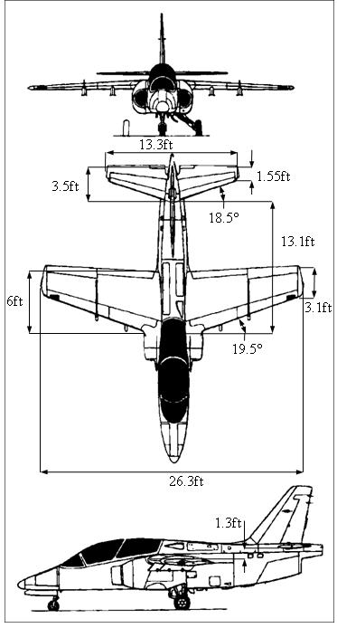
Figure SP3.7.1 - 3D View of the Cessna T-37 and SIAI S-211 Aircraft (Source: http://www.aviastar.org/index2.html)

Although they are used for the same purpose, the two aircraft have different weight and somewhat different dimensions, with the Cessna T-37 having a larger weight and, therefore, a larger wing surface and a larger wing span. The values of the stability derivatives , Lmcc  , for the 2 aircraft are summarized in the Tables below.

Table SP3.7.1 - , Lmcc  at different flight conditions for the Cessna T-37

SIAI S-211 APPROACH CRUISE (LOW) CRUISE (HIGH)



Table SP3.7.2 - , Lmcc  at different flight conditions for the SIAI S-211

Considering that the cruise speed for the SIAI S-211 aircraft is higher than the cruise speed for the Cessna T-37 the two aircraft have a similar L c  The substantially larger (negative) value of m c  for the Cessna T-37 aircraft is due to the larger moment arm () H ACCGxx for this aircraft compared to the SIAI S211 (although the wing sweep angle on the SIAI S211 is rather limited).

Short Problem 3.8

Repeat Short Problem 3.7 for the following longitudinal control derivatives:

E Lc  , E m c 

Note that the Cessna T-37 aircraft only features elevators and does not feature stabilators.

Solution of Short Problem 3.8

The drawings of the Cessna T-37 and SIAS Marchetti S-211 are shown below.

Figure SP3.8.1 - 3D View of the Cessna T-37 and SIAI S-211 Aircraft (Source: http://www.aviastar.org/index2.html)

The value of the stability derivatives E Lc  , E m c  for the 2 aircraft is summarized below.

Table SP3.8.1E Lc  , E m c  at different flight conditions for the Cessna T-37

SIAI S-211 APPROACH

Table SP3.8.2E Lc  , E m c  at different flight conditions for the SIAI S-211

As shown in the top view in the above drawings, the horizontal tail surface and, therefore, the elevator surface of the Cessna T-37 aircraft are larger than those of the SIAI S-211 aircraft. This explains the slightly larger value of E Lc  for the Cessna T-37.

Additionally, as also discussed in Short Problem 3.7, the Cessna T-37 aircraft features a larger moment arm () H ACCGxx than the SIAI S-211 aircraft. Therefore, due to a slightly larger force coefficient and a larger moment arm, the absolute value of E m c  for the Cessna T-37 aircraft is larger than the value for the SIAI S-211, despite the fact that the cruise Mach value for the SIAI S-211 is higher than the cruise Mach value for the Cessna T-37.

Short Problem 3.9

Repeat Short Problem 3.7 for the following longitudinal stability derivatives:

,,, qqLmLm cccc

Solution of Short Problem 4.9

The drawings of the Cessna T-37 and SIAS Marchetti S-211 are shown below.

Figure SP3.9.1 - 3D View of the Cessna T-37 and SIAI S-211 Aircraft (Source: http://www.aviastar.org/index2.html)

The values of the stability derivatives ,,, qqLmLm cccc

for the 2 aircraft are summarized below.

T-37 CLIMB CRUISE APPROACH

Derivatives

Table SP3.9.1 - ,,, qqLmLm cccc  at different flight conditions for the Cessna T-37

SIAI S-211 APPROACH CRUISE (LOW) CRUISE (HIGH)

Derivatives

Table SP3.9.2 - ,,, qqLmLm cccc  at different flight conditions for the SIAI S-211

An objective and accurate comparative analysis for the stability derivatives ,,, qqLmLm cccc  might not be possible with the available aerodynamic data. In fact, while it is true that the values of the derivatives ,,, qqLmLm cccc  for the SIAI S-211 aircraft are larger than the values for Cessna T-37 aircraft, it is also true that this trend might be due to the larger Mach number, and therefore, larger value of H L c  . On the other side, at the same Mach number, it might be speculated that the ,,, qqLmLm cccc  for the Cessna T-37 aircraft should be slightly higher than the values for the SIAI S-211 due to the issues discussed below (slightly smaller horizontal tail and smaller moment arm () H ACCGxx ).

Problems for Chapter IV

Problem 4.1

Consider the data relative to the McDonnell Douglas DC 8 aircraft in Appendix C. Use the provided drawings to extract all the relevant geometric characteristics of the aircraft. Using the modeling approach outlined in this chapter, the so-called dihedral effect l c  can be modeled as:

Estimate the value of lc  for this aircraft. Also, evaluate the percentage of each of the different contributions with respect to the total l c  value.

Solution of Problem 4.1

All the relevant geometric parameters used in this problem were extracted from the images in Appendix C. From the drawings in Appendix C, the following geometric parameters were identified:

2 221.943.8,6.2,18.7,400.698

Note that 2V b is actually the same of the span of the vertical tail; this value is used so that the geometric parameters of the vertical tail can be found in a similar manner as the parameters for the wing. Next, using the assumption of straight wings, the vertical tail geometric parameters were derived using the values from the drawings in Appendix C.

Vertical Tail Geometric Parameters

The following vertical tail parameters are required to determine the stability derivatives.

Again, it should be emphasized that 2V S is twice the value of the area of the vertical tail; however, the use of 2V S allows finding the following geometric parameters:

Wing-Tail Geometric Parameters

The distances SVX , SVZ , SR X and SRZ are given by:

Technically speaking the parameters SR X and SRZ - relative to the rudder – are not needed in this problem. However, they were reported since they are conceptually similar to SVX and SVZ

Vertical Tail Lift Slope Coefficient

This coefficient is calculated using the Polhamus formula with effVAR , defined as

The parameter 1c is found from Figure 4.15 using 0.3322 V   along with the parameter:

Using 0.332 V   and 1 21.203 V br  Figure 4.15 provides 1 1.575 c  .

Next, the parameter 2c is found from Figure 4.16 using:

The geometric parameter HVACx

, shown in Figure 4.17, is calculated using:

Note that HZ is considered negative when above the CG. Using the above HVACx  value,

Figure 4.16 provides 2 0.973 c  . Finally, using HVSS in Figure 4.18, we would have:

leading to:

Using 5.3744 effVAR  , the application of the Polhamus formula leads to:

Since the values of the sweep angle and the tip ratio are outside the ranges of validity for the Polhamus range, it is reasonable to expect that the above estimate exceeds substnatially the ‘true’ value. Therefore, considering a 20% overestimate, the value of

is considered instead.

Wing and Body Contribution.

The modeling for WB lc  is given by:

Next, the following individual contributions to the dihedral effect in the above relationship are evaluated separately.

- wing contribution due to the geometric dihedral angle;

- wing contribution due to the wing-fuselage positions;

- wing contribution due to the sweep angle;

- wing contribution due to the aspect ratio;

- wing contribution due to the twist angle;

- body (fuselage) contribution.

(1) Wing contribution to the Dihedral effect due to the geometric dihedral angle.

Using 0.251  and 0.5

Figure 4.44 provides 1.147 MK

 . Therefore:

(2) Wing contribution to the Dihedral effect due to wing-fuselage position

The fuselage’s diameter Bd is required for the evaluation of this term. Bd is found using:

where AVGf S is the average cross-sectional area of the fuselage calculated using:

where the average height and width of the fuselage were obtained from the drawings in Appendix C. Therefore, we have:

leading to the following

(3) Wing contribution to the Dihedral effect due to wing sweep angle

The value of 1Lc is required to calculated WB Wing l

c  . This value is calculated using the given flight conditions and data from Standard Atmosphere Tables:

(4) Wing contribution to the Dihedral effect due to wing aspect ratio

Using 0.251  and 7.323 AR  Figure 4.42 provides:

(5) Wing contribution to the Dihedral effect due to wing twist angle

Due to a lack of specific information, the twist angle is assumed to be 20.0345 W 

Using 0.251  and

/4 /4

(6) Fuselage contribution to the Dihedral effect

This contribution is given by:

Adding together the previous contributions we would

0.06890.0150.05900.002380.0080.123

Horizontal Tail Contribution.

This contribution is non negligible for this aircraft since it has a non negligible dihedral angle along with a substantial sweep angle.

(1) Horizontal tail contribution to the Dihedral effect due to the geometric dihedral angle.

Using 0.444  and 0.5 32.7  Figure 4.43 provides: 

20.0001571/deg

Figure 4.44 provides 1.09 MK   . Therefore:

(2) Horizontal

Adding the previous contributions we would have:

The above value provides the contribution of the horizontal tail assumed to be as a wing. Due to the smaller size and lower wing span, the ‘true’ dihedral contribution from the horizontal is found using:

Vertical Tail Contribution.

The value of this contribution is given by:

Table P4.1.1 shows the percentage of each of the coefficients with respect to the total

l c  value. Term

Wing contribution due to the geometric dihedral angle

Wing contribution due to the wing-fuselage position 0.015 -8.0 %

Wing contribution due to the sweep angle

31.4 %

Wing contribution due to the aspect ratio 0 0.0 %

Wing contribution due to the twist angle

Body (fuselage) contribution

1.3 %

Table P4.1.1 - Percentage of each of the contributions to the total l c  value.

Problem 4.2

Consider the data relative to the McDonnell Douglas DC 8 aircraft in Appendix C. Use the provided drawings to extract all the relevant geometric characteristics of the aircraft. Using the modeling approach outlined in this chapter, provide estimates for the following stability derivatives: , Yncc 

For both aerodynamic parameters highlight the contribution of the vertical tail vs. the total value.

Solution of Problem 4.2

All the relevant geometric parameters used in this problem were extracted from the images in Appendix C.

Calculation of Y c 

The general modeling of this derivative is given by:

Wing Contribution . W Yc  is given by:

Body Contribution . B Yc  is given by:

As described in Section 4.2.2 PVS  is the cross section at the location of the fuselage where the flow transitions from potential to viscous. From the drawings in Appendix C, using the approach described in Section 4.2.2

Therefore:

Therefore, we would have:

have been found in the previous problem.

Finally, the total value of Yc  is given by:

Calculation of n c

The general modeling of this derivative is:

It is easy to visualize that the both the wing and the horizontal tail will not provide a significant contribution to n c  . Therefore, we would have:

Body Contribution

To obtain N K from Figure 4.68 the following parameters from Figure 4.67 related to dimensions of the DC-8 aircraft from Appendix C are required.

Using the above parameters Figure 4.68 provides: 0.0019 NK  Next, the following parameter is required to obtain Re l K .

The values of the speed of sound and the kinematic viscosity were obtained from the Standard Atmosphere Tables, using the given flight altitude. Finally, using ReFuselage , Figure 4.69 provides Re 2.18 l K  leading to:

1660.21146.61 57.357.30.00192.180.146 2773142.5 S Bl

Vertical Tail Contribution

is given by:

VX and VZ were calculated in P4.1

Thus, the total value of n c  is given by,

Problem 4.3

Consider the data relative to the McDonnell Douglas DC 8 aircraft in Appendix C. Use the provided drawings to extract all the relevant geometric characteristics of the aircraft. Using the modeling approach outlined in this chapter, provide estimates for the following control derivatives:  ,, RRR Yln ccc 

Solution of Problem 4.3

All the relevant geometric parameters used in this problem were extracted from the drawings in Appendix C.

Calculation of R Yc 

The modeling of R Yc  is given by:

where V Lc  was found and shown in P4.1. To find   RK  the parameters I and F and their associated RK (shown in Section 4.2.4, Figure 4.27) are required. Using 0.332 V   , Figure 4.27 provides:

Using 4.6 0.34 13.5 Rudder VertTail c c  from the drawings in Appendix C, Figure 4.26 provides: 0.559 R 

Finally, the value of R Yc  is given by:

Calculation of

The modeling of

is given by:

where R X and RZ were found and shown in P4.1.

Calculation

The modeling of R n c  is given by:

Calculation

0.5470.309

Problem 4.4

Consider the data relative to the McDonnell Douglas DC 8 aircraft in Appendix C. Use the provided drawings to extract all the relevant geometric characteristics of the aircraft. Using the modeling approach outlined in this chapter, provide estimates for the following stability derivatives:

 , prlncc

Solution of Problem 4.4

All the relevant geometric parameters used in this problem were extracted from the drawings in Appendix C.

Calculation of p l c

As shown in Section 4.6.3, the modeling for p l c is given by:

WB lpc is given by WBWlplp k ccRDP   where 0.661   , 0.597 k  (from P4.3).

The parameters 8.116 AR k   and 41.9   (from P4.3) are needed to evaluate RDP .

Using the above parameters, along with 0.251  , the use of Figure 4.80 and 4.81 provides 0.386 RDP  , leading to: 0.597 0.3860.348 0.661 WBWlplp k ccRDP

The contribution from the horizontal is given by:

where

W H lpH H H k cRDP 

. It should be clear that this contribution is expected to be negligible due to the small values of 2 , HHSb Sb

. The parameters , HHk  are given by:

Finally,

The contribution from the vertical is given by:

Finally the total value of lpc is given by:

Calculation of

As shown in Section 4.6.7, the modeling for r n c is given by:

Using Figure 4.89 with 0.251  , 7.323

 , /4 30.7 c  and 0.4240.320.104 ACCGxx . The calculation of ACx is shown in chapter II. We will have:

A relationship for Vnr c is given by:

Thus, the total value of r n c is given by:

rrrWV nnn ccc

Problem 4.5

Consider the data relative to the Aeritalia G91 aircraft in Appendix C. Use the provided drawings to extract all the relevant geometric characteristics of the aircraft. Using the modeling approach outlined in this chapter, the so-called dihedral effect l c  can be modeled as:

Estimate the value of lc  for this aircraft. Also, evaluate the percentage of each of the different contributions with respect to the total l c  value.

Solution of Problem 4.5

All the relevant geometric parameters used in this problem were extracted from the images in Appendix C. Also, note that several geometric parameters related to the wing and the horizontal tail were calculated previously for the Aeritalia G91 problems in chapter II and chapter III. From the drawings in Appendix C, the following geometric parameters were identified: 2 25.611.2,2.2,7.3,500.873

Vertical Tail Geometric Parameters

The following vertical tail parameters are required to determine the stability derivatives.

Again, it should be emphasized that 2V S is twice the value of the area of the vertical tail; however, the use of 2V S allows finding the following geometric parameters:

Wing-Tail Geometric Parameters

The distances SVX , SVZ , SR X and SRZ are evaluated using the procedure shown in SSP4.2. They are needed to determine the stability derivatives related with the vertical tail and the rudder. They are given by:

Technically speaking the parameters SR X and SRZ - relative to the rudder – are not needed in this problem. However, they were reported since they are conceptually similar to SVX and SVZ .

Vertical Tail Lift Slope Coefficient

This coefficient is calculated using the Polhamus Formula with effVAR , defined as

The parameter 1c is found from Figure 4.15 using 0.301 V   along with the parameter:

Using 0.301 V   and 1 20.778 V br  Figure 4.15 provides 1 1.382 c  .

Next, the parameter 2c is found from Figure 4.16 using:

The geometric parameter HVACx  , shown in Figure 4.17, is calculated using:

Note that HZ is considered negative when above the CG. Using the above HVACx  value,

Figure 4.16 provides 2 0.992 c  . Finally, using HVSS in Figure 4.18, we would have:

Using 3.2284 effVAR  , the application of the Polhamus formula leads to:

Wing and Body Contribution.

Next, the following individual contributions to the dihedral effect in the above relationship are evaluated separately.

- wing contribution due to the geometric dihedral angle; - wing contribution due to the wing-fuselage positions;

- wing contribution due to the sweep angle;

- wing contribution due to the aspect ratio;

- wing contribution due to the twist angle; - body (fuselage) contribution.

(1) Wing contribution to the Dihedral effect due to the geometric dihedral angle.

Using 0.506  and 0.5 35.3  Figure 4.43 provides:

 20.000161/deg

Figure 4.44 provides 1.032

Therefore:

(2) Wing contribution to the Dihedral effect due to wing-fuselage position

The fuselage’s diameter Bd is required for the evaluation of this term. Bd is found using:

where AVGf S is the average cross-sectional area of the fuselage calculated using:

where the average height and width of the fuselage were obtained from the drawings in Appendix C. Therefore, we have:

leading to the following value for /

(3) Wing contribution to the Dihedral effect due to wing sweep angle

The value of 1Lc is required to calculated

. This value is calculated using the given flight conditions and data from Standard Atmosphere Tables:

(4) Wing contribution to the Dihedral effect due to wing aspect ratio

Using

(5) Wing contribution to the Dihedral effect due to wing twist angle

Due

(6) Fuselage contribution to the Dihedral effect

This contribution is given by:

Adding together the previous contributions we would

Horizontal Tail Contribution.

Since the horizontal tail of this aircraft does not have significant dihedral or anhedral angles, we can assume that: 0

Vertical Tail Contribution.

The value of this contribution is given by:

Thus,

Note that for this aircraft we assume 1 20.035rad

Therefore, the final total estimated value of l c

Table P4.5.1 shows the percentage of each of the coefficients with respect to the total l c  value.

Wing contribution due to the geometric dihedral angle

Wing contribution due to the wing-fuselage position 0.034 -20.7 %

Wing contribution due to the sweep angle -0.069 42.7 %

Wing contribution due to the aspect ratio -0.028 17.1 %

Wing contribution due to the twist angle

Body (fuselage) contribution

Horizontal tail contribution 0

1.5 %

Table P4.5.1. Percentage of each of the contributions to the total l c  value.

Problem 4.6

Consider the data relative to the Aeritalia G91 aircraft in Appendix C. Use the provided drawings to extract all the relevant geometric characteristics of the aircraft. Using the modeling approach outlined in this chapter, provide estimates for the following stability derivatives: , Yncc 

For both aerodynamic parameters highlight the contribution of the vertical tail vs. the total value.

Solution of Problem 4.6

All the relevant geometric parameters used in this problem were extracted from the images in Appendix C. Also, note that several geometric parameters related to the wing, horizontal tail, and vertical tail were calculated previously for the G91 problems in chapter II, chapter III, and in P4.5.

Calculation of Y c 

The general modeling of this derivative is given by:

Wing Contribution

Body Contribution

Horizontal Tail Contribution. H Yc  is found using:

Since 0 H 

Vertical Tail Contribution. V

c  is found using:

Therefore, we would have:

Finally, the total value of Yc  is given by:

Calculation of n c

The general modeling of this derivative is:

nnnnn ccccc  

It is easy to visualize that the both the wing and the horizontal tail will not provide a significant contribution to n c  . Therefore, we would have:

Body Contribution B n c  is given by: 57.3 S Bl B B nNR S l cKK Sb  

To obtain N K from Figure 4.68 the following parameters from Figure 4.67 related to dimensions of the G91 aircraft from Appendix C are required.

Using the above parameters Figure 4.68 provides: 0.00241 NK  Next, the following parameter is required to obtain Re l K .

Vertical Tail Contribution

is given by:

VX and VZ were calculated in P4.5.

Thus, the total value of n c  is given by:

Problem 4.7

Consider the data relative to the Aeritalia G91 aircraft in Appendix C. Use the provided drawings to extract all the relevant geometric characteristics of the aircraft. Using the modeling approach outlined in this chapter, provide estimates for the following control derivatives:  ,, RRR Yln ccc 

A l c 

Solution of Problem 4.7

All the relevant geometric parameters used in this problem were extracted from the drawings in Appendix C. Additionally, all the geometric parameters related to the wing and the horizontal and vertical tail were calculated previously in the G91 problems solved in chapter II, chapter III, and in P4.5.

Calculation of R Yc 

The modeling of R Yc  is given by:

where V Lc  was found and shown in P4.5. To find   RK  the parameters I and F and their associated RK (shown in Section 4.2.4, Figure 4.27) are required. Using 0.301 V   , Figure 4.27 provides:

Using 1.2 0.23 5.21 Rudder VertTail c c  from the drawings in Appendix C, Figure 4.26 provides: 0.429 R 

Finally, the value of R Yc  is given by:

Calculation of R lc 

The modeling of R lc  is given by:

where R X and RZ were found and shown in P4.9.

Calculation of R n c

The modeling of R n c  is given by:

Calculation of

As shown in Section 4.3.3, the following parameters are required for the modeling of

Finally, the value of A

Problem 4.8

Consider the data relative to the Aeritalia G91 aircraft in Appendix C. Use the provided drawings to extract all the relevant geometric characteristics of the aircraft. Using the modeling approach outlined in this chapter, provide estimates for the following stability derivatives:  ,, ppp Ylnccc  ,, rrr Ylnccc

Solution of Problem 4.8

Calculation of p Y c

As shown in Section 4.6.2, the modeling for p Y c is given by:

where V Yc  was found in P4.6 while VX and VZ were shown in P4.5

Calculation of p l c

As shown in Section 4.6.3, the modeling for p l c is given by:

The parameters 7.194 AR k   and 41.9   (from P4.7) are needed to evaluate RDP .

Using the above parameters, along with 0.506  , the use of Figure 4.80 and 4.81 provides 0.395 RDP  , leading to:

The contribution from the horizontal is given by:

where

. It should be clear that this contribution is expected to be negligible due to the small values

. The parameters , HHk  are given by:

Finally,

The

where V Yc  was obtained from P4.6. Finally the total value of lpc is given by:

Calculation of p n c

As shown in Section 4.6.4, the modeling for p n c is given by:

The contribution from the wing is given by:

As shown in Section 4.6.4, the coefficient

Next, using 0.506

Assuming

, Figure 4.83 provides:

The contribution from the vertical tail is given by:

where the value of V

was found in P4.6. Finally the total value of np c is:

Calculation

As shown in Section 4.6.5, the modeling for r

Calculation of r

Next, using Figure 4.85 with the parameters

Next,

Adding the previous terms, the value of W

Thus,

Calculation of r n c

1 0.1850.0960.280 WVlrlrlr ccc rad

As shown in Section 4.6.7, the modeling for r n c is given by:

Using Figure 4.89 with 0.506  , 4.525 AR  , /4 38 c  and 0.3270.260.067

A relationship for Vnr c is given by:

Thus, the total value of

Problem 4.9

Estimate the value of lc  for this aircraft. Also, evaluate the percentage of each of the different contributions with respect to the total l c  value. Next, compare the obtained l c  value with the TRUE value listed in Appendix B (Aircraft #3) and evaluate the errors associated with the use of the ‘empirical’ modeling approach.

Solution of Problem 4.9

All the relevant geometric parameters used in this problem were extracted from the images in Appendix C. Also, note that several geometric parameters related to the wing and the horizontal tail were calculated previously for the Beech B99 problems in chapter II and chapter III. From the drawings in Appendix C, the following geometric parameters were identified:

2 26.813.6,3.6,8.2,470.820

Vertical Tail Geometric Parameters

The following vertical tail parameters are required to determine the stability derivatives.

Again, it should be emphasized that 2V S is twice the value of the area of the vertical tail; however, the use of 2V S allows finding the following geometric parameters:

Wing-Tail Geometric Parameters

The distances SVX , SVZ , SR X and SRZ are evaluated as in SSP4.2. They are needed to determine the stability derivatives related with the vertical tail and the rudder. They are given by:

Technically speaking the parameters SR X and SRZ - relative to the rudder – are not needed in this problem. However, they were evaluated since they are conceptually similar to SVX and SVZ .

Vertical Tail Lift Slope Coefficient

This coefficient is calculated using the Polhamus Formula with effVAR , defined as

The parameter 1c is found from Figure 4.15 using 0.439 V   along with the parameter:

Using 0.439 V   and 1 21.172 V br  Figure 4.15 provides 1 1.566 c  .

Next, the parameter 2c is found from Figure 4.16 using:

The geometric parameter HVACx  , shown in Figure 4.17, is calculated using:

Note that HZ is considered negative when above the CG. Using the above HVACx  value,

Figure 4.16 provides 2 0.866 c  . Finally, using HVSS in Figure 4.18, we would have:

Using 3.0144 effVAR  , the application of the Polhamus formula leads to:

Since the sweep angle, the aspect ratio, the tip ration and Mach number are well within the range of validity of the Polhamus formula, it is reasonable to expect that the above estimate is correct.

Wing and Body Contribution.

The modeling for WB lc  is given by:

Next, the following individual contributions to the dihedral effect in the above relationship are evaluated separately.

- wing contribution due to the geometric dihedral angle;

- wing contribution due to the wing-fuselage positions;

- wing contribution due to the sweep angle;

- wing contribution due to the aspect ratio;

- wing contribution due to the twist angle;

- body (fuselage) contribution.

(1) Wing contribution to the Dihedral effect due to the geometric dihedral angle. Using

Figure 4.44 provides 1.021

. Therefore:

(2) Wing contribution to the Dihedral effect due to wing-fuselage position

The fuselage’s diameter Bd is required for the evaluation of this term. Bd is found using:

where AVGf S is the average cross-sectional area of the fuselage calculated using:

where the average height and width of the fuselage were obtained from the drawings in Appendix C. Therefore, we have:

leading to the following

(3) Wing contribution to the Dihedral effect due to wing sweep angle

The value of 1Lc is required to calculated WB Wing l

c  . This value is calculated using the given flight conditions and data from Standard Atmosphere Tables:

(4) Wing contribution to the Dihedral effect due to wing aspect ratio

Using 0.459  and 7.557 AR  Figure 4.42 provides:

(5) Wing contribution to the Dihedral effect due to wing twist angle

Due to a lack of specific information, the twist angle is assumed to be 20.0345 W 

(6) Fuselage contribution to the Dihedral effect

This contribution is given by:

Adding

0.06810.0280.0030.0030.000010.0120.052

Horizontal Tail Contribution.

This contribution is non negligible for this aircraft since it has a non negligible dihedral angle along with a substantial sweep angle.

(1) Horizontal tail contribution to the Dihedral effect due to the geometric dihedral angle.

Using 0.544  and 0.5 15  Figure 4.43 provides: 

20.0001571/deg

Figure 4.44 provides 1.013 MK   . Therefore:

(2)

Adding the previous contributions we would have:

Vertical Tail Contribution.

The value of this contribution is given by:

Thus,

0.580.24280 0.7243.060.40.0097.5571.224 1cos0.0034.1

Note that for this aircraft

  at low cruise conditions (see Appendix B, Aircraft #3).

Therefore, the final total estimated value of l c  for the B99 aircraft is:

Table P4.9.1 shows the percentage of each of the coefficients with respect to the total l c  value.

Wing contribution due to the geometric dihedral angle

Wing contribution due to the wing-fuselage position

Wing contribution due to the sweep angle

Wing contribution due to the aspect ratio

Wing contribution due to the twist angle

Body

0.0

Table P4.9.1. Percentage of each of the contributions to the total l c  value.

The above Table suggests that the total dihedral effect is approximately equally divided among the contribution from the wing geometric dihedral angle and the dihedral effect of the vertical tail. The remaining positive dihedral effects cancel out with the negative dihedral effect due to the wing-fuselage position.

Comparison between TRUE Values and ‘Empirical’ Values

A comparison between the true value of l c  and its estimate using the ‘empirical’ aerodynamic modeling approach, along with a calculation of the percentage of the error, is shown in the Table below:

Table P4.9.2 - Comparative analysis with percentages of the error

The above result suggests that the mathematical modeling for the dihedral effect for this aircraft provides accurate results.

Problem 4.10

For both aerodynamic parameters highlight the contribution of the vertical tail vs. the total value. Next, compare the obtained values with the TRUE values listed in Appendix B (Aircraft #3) and evaluate the errors associated with the use of the ‘empirical’ modeling approach.

Solution of Problem 4.10

All the relevant geometric parameters used in this problem were extracted from the images in Appendix C. Also, note that several geometric parameters related to the wing, horizontal tail, and vertical tail were calculated previously for the B99 problems in chapter II, chapter III, and in P4.9.

Calculation of Y c

The general modeling of this derivative is given by:

Horizontal Tail Contribution.

is found using:

Vertical Tail Contribution.

is found using:

have been found in the previous problem.

Therefore, we would have:

Finally,

Calculation of

It is easy to visualize that the both the wing and the horizontal tail will not provide a significant contribution to n c  . Therefore, we would have:

Body Contribution B

is given by:

To obtain N K from Figure 4.68 the following parameters from Figure 4.67 related to dimensions of the B99 aircraft from Appendix C are required.

Using the above parameters Figure 4.68 provides: 0.0017 NK  Next, the following parameter is required to obtain Re l K .

A close-look at the drawings in Appendix C for the Beech 99 shows that this aircraft features some large and long nacelles for the engines under the wing. Since these engines are located somewhat in front of the center of the gravity, the previously calculated

B n c  value is multiplied by a 1.2 correction factor, leading to 0.141 B n c

Vertical Tail Contribution V n c  is given by:

VX and VZ were calculated in P4.9.

Thus, the total value of n c  is given by,

0.1410.2240.083

Comparison between TRUE Values and ‘Empirical’ Values

A comparison between the true value of Yc  and n c  and their estimates along with a calculation of the percentage of the error, is shown in the Table below:

Table P4.10.1 - Comparative analysis with percentages of the error

The results in the above Table suggest a very desirable accuracy for the calculation of the above aerodynamic coefficients.

Problem 4.11

, prlncc

Next, compare the obtained values with the TRUE values listed in Appendix B (Aircraft #3) and evaluate the errors associated with the use of the ‘empirical’ modeling approach.

Solution of Problem 4.11

All the relevant geometric parameters used in this problem were extracted from the drawings in Appendix C. Additionally, all the geometric parameters related to the wing and the horizontal and vertical tail were calculated previously in the B99 problems solved in chapter II, chapter III, and in P4.9.

Calculation of p l c

As shown in Section 4.6.3, the modeling for p l c is given by:

The parameters 9.045 AR k

 and 0.2

(from P4.11) are needed to evaluate RDP

Using the above parameters, along with 0.459  , the use of Figure 4.80 and 4.81 provides 0.506 RDP

, leading to:

The contribution from the horizontal is given by:

Finally

Calculation of r n c

As shown in Section 4.6.7, the modeling for r n c is given by:

A relationship for rW

Using Figure 4.89 with

Thus, the total value of r n c is given by:

Comparison between TRUE Values and ‘Empirical’ Values

A comparison between the true value of , prlncc and their estimates along with a calculation of the percentage of the error is shown in the Table below.

Table P4.11.1 - Comparative analysis with percentages of the error

The above results suggest that the above important aerodynamic coefficients have been estimated with a desirable level of accuracy.

Problem 4.12

Estimate the value of lc  for this aircraft. Also, evaluate the percentage of each of the different contributions with respect to the total l c  value. Next, compare the obtained l c  value with the TRUE value listed in Appendix B (Aircraft #4) and evaluate the errors associated with the use of the ‘empirical’ modeling approach.

Solution of Problem 4.12

All the relevant geometric parameters used in this problem were extracted from the images in Appendix C. Also, note that several geometric parameters related to the wing and the horizontal tail were calculated previously for the Cessna T37 problems in chapter II and chapter III. From the drawings in Appendix C, the following geometric parameters were identified:

2 24.89.6,2.5,6,330.576

Vertical Tail Geometric Parameters

The following vertical tail parameters are required to determine the stability derivatives. 2.5 0.417 6 V V T V R c c

2 2 2 9.6

Again, it should be emphasized that 2V S is twice the value of the area of the vertical tail; however, the use of 2V S allows finding the following geometric parameters:

Wing-Tail Geometric Parameters

The distances SVX , SVZ , SR X and SRZ are evaluated as in SSP4.2. They are needed to determine the stability derivatives related with the vertical tail and the rudder. They are given by:

Technically speaking the parameters SR X and SRZ - relative to the rudder – are not needed in this problem. However, they were evaluated since they are conceptually similar to SVX and SVZ .

Vertical Tail Lift Slope Coefficient

This coefficient is calculated using the Polhamus Formula with effVAR , defined as

The parameter 1c is found from Figure 4.15 using 0.346 V   along with the parameter:

Using 0.417 V   and 1 21.091 V br  Figure 4.15 provides 1 1.535 c  .

Next, the parameter 2c is found from Figure 4.16 using:

The geometric parameter HVACx  , shown in Figure 4.17, is calculated using:

Note that HZ is considered negative when above the CG. Using the above HVACx  value,

Figure 4.16 provides 2 0.871 c  . Finally, using HVSS in Figure 4.18, we would have:

Using 2.9274 effVAR  , the application of the Polhamus formula leads to:

Wing and Body Contribution.

Next, the following individual contributions to the dihedral effect in the above relationship are evaluated separately.

- wing contribution due to the geometric dihedral angle; - wing contribution due to the wing-fuselage positions; - wing contribution due to the sweep angle; - wing contribution due to the aspect ratio;

- wing contribution due to the twist angle;

- body (fuselage) contribution.

(1) Wing contribution to the Dihedral effect due to the geometric dihedral angle.

Using

provides

 . Therefore:

(2) Wing contribution to the Dihedral effect due to wing-fuselage position

The fuselage’s diameter Bd is required for the evaluation of this term. Bd is found using:

where AVGf S is the average cross-sectional area of the fuselage calculated using:

where the average height and width of the fuselage were obtained from the drawings in Appendix C. Therefore, we have:

leading to the following value for / WB l Highlow wing c  :

It turns out that for this aircraft / 0

Figure 4.45.

(3) Wing contribution to the Dihedral effect due to wing sweep angle

The value of 1Lc is required to calculated

See

Wing

sweep angle c  . This value is calculated using the given flight conditions and data from Standard Atmosphere Tables:

1 f K  . Therefore:

It turns out that this contribution is positive due to the low wing sweep angle.

(4) Wing contribution to the Dihedral effect due to wing aspect ratio

Using 0.726  and 6.277 AR  Figure 4.42 provides:

(5) Wing contribution to the Dihedral effect due to wing twist angle

Due to a lack of specific information, the twist angle

(6) Fuselage contribution to the Dihedral effect

This

Adding together the previous contributions we would have:

Horizontal Tail Contribution.

Since the horizontal tail of this aircraft does not have significant dihedral or anhedral angle, we have the condition: 0 H lc 

Vertical Tail Contribution.

The value of this contribution is given by:

Table P4.12.1 shows the percentage of each of the coefficients with respect to the total l c  value.

Wing contribution due to the geometric dihedral angle

Wing contribution due to the wing-fuselage position 0 0.0 %

Wing contribution due to the sweep angle 0.002 -3.0 %

Wing contribution due to the aspect ratio

Wing contribution due to the twist angle

Body (fuselage) contribution

( l c  )

Table P4.12.1. Percentage of each of the contributions to the total l c  value.

Comparison between TRUE Values and ‘Empirical’ Values

Table P4.12.2 - Comparative analysis with percentages of the error The above result suggests that for this aircraft the mathematical modeling provides only an approximated estimate of this important aerodynamic coefficient.

Problem 4.13

For both aerodynamic parameters highlight the contribution of the vertical tail vs. the total value. Next, compare the obtained values with the TRUE values listed in Appendix B (Aircraft #4) and evaluate the errors associated with the use of the ‘empirical’ modeling approach.

Solution of Problem 4.13

All the relevant geometric parameters used in this problem were extracted from the images in Appendix C. Also, note that several geometric parameters related to the wing, horizontal tail, and vertical tail were calculated previously for the Cessna T37 problems in chapter II, chapter III, and in P4.12

Calculation of Y c

The general modeling of this derivative is given by:

Horizontal Tail Contribution. H Yc  is also assumed to be negligible since this aircraft does not have a geometric dihedral angle for the horizontal tail.

Vertical Tail Contribution. V Yc  is found using:

Using 1 1.091 2 Vb

 Figure 4.13 provides 0.761 VYk  . The term 1 V

Finally,

has been found in the previous problem. Therefore, we would have:

Calculation of n c

The general modeling of this derivative is: WBHV nnnnn ccccc 

It is easy to visualize that the both the wing and the horizontal tail will not provide a significant contribution to n c  for this aircraft. Therefore, we would have: BVnnn ccc

Body Contribution B n c  is given by: 57.3 S Bl B B nNR S l cKK Sb  

To obtain N K from Figure 4.68 the following parameters from Figure 4.67 related to dimensions of the Cessna T37 aircraft from Appendix C are required.

Using the above parameters Figure 4.68 provides: 0.00038 NK  Next, the following parameter is required to obtain Re l K .

cKK Sbrad

Vertical Tail Contribution V

is given by:

VX and VZ were shown also in P4.12

Thus, the total value of n c  is given by,

Comparison between TRUE Values and ‘Empirical’ Values

A comparison between the true value of Yc  and n c  and their estimates along with a calculation of the percentage of the error, is shown in the Table below:

Table P4.13.1 - Comparative analysis with percentages of the error

The results in the above Table indicate a poor overall modeling of these important derivatives.

Problem 4.14

,, RRR Yln ccc 

Next, compare the obtained values with the TRUE values listed in Appendix B (Aircraft #4) and evaluate the errors associated with the use of the ‘empirical’ modeling approach.

Solution of Problem 4.14

All the relevant geometric parameters used in this problem were extracted from the drawings in Appendix C. Additionally, all the geometric parameters related to the wing and the horizontal and vertical tail were calculated previously in the Cessna T37 problems solved in chapter II, chapter III, and in P4.13.

Calculation of R Yc 

The modeling of R Yc  is given by:

where V Lc  was found and shown in P4.12. To find   RK  the parameters I and F and their associated RK (shown in Section 4.2.4, Figure 4.27) are required. Using 0.417 V   , Figure 4.27 provides:

Using 1.4 0.31 4.49

Rudder VertTail c c  from the drawings in Appendix C, Figure 4.26 provides:

Finally, the value of R

Calculation of R lc 

The modeling of R lc  is given by:

where R X and RZ were also shown in P4.13.

Calculation of

The modeling of R n c

is given by:

Calculation of A

As shown in Section 4.3.3, the following parameters are required for the modeling of A

Finally, the value of A

Comparison between TRUE Values and ‘Empirical’ Values

A comparison between the true value of ,,, RRRA Ylnl cccc  and their estimates using the ‘empirical’ aerodynamic modeling approach, along with a calculation of the percentage of the error, is shown in the Table below.

Table P4.14.1 Comparative analysis with percentages of the error

The above results point out a limited accuracy of the modeling for the above derivatives.

Problem 4.15

 ,, ppp Ylnccc  ,, rrr Ylnccc

Next, compare the obtained values with the TRUE values listed in Appendix B (Aircraft #4) and evaluate the errors associated with the use of the ‘empirical’ modeling approach.

Solution of Problem 4.15

All the relevant geometric parameters used in this problem were extracted from the drawings in Appendix C. Additionally, all the geometric parameters related to the wing and the horizontal and vertical tail were calculated previously in the Cessna T37 problems solved in chapter II, chapter III, and in P4.12.

Calculation of p Y c

As shown in Section 4.6.2, the modeling for p Y c is given by:

where V Yc

was found in P4.14 while VX and VZ were shown in P4.12.

Calculation of p l c

As shown in Section 4.6.3, the modeling for p l c is given by:

WB lpc is given by WBWlplp k ccRDP   where 0.888   , 0.734 k  (from P4.15).

The parameters 7.594 AR k   and 0.1   (from P4.15) are needed to evaluate RDP .

Using the above parameters, along with 0.726  , the use of Figure 4.80 and 4.81 provides 0.483 RDP  , leading to:

The contribution from the horizontal is given by:

. It should be clear that this contribution is expected to be negligible due to the small values of

. The parameters , HHk  are given by:

Finally, the following parameters are required to obtain HRDP

The contribution from the vertical is given by:

where V Yc

Finally the

was obtained from P4.13

of lpc is given by:

Calculation of p n c

As shown in Section 4.6.4, the modeling for p n c is given by:

The contribution from the wing is given by:

As shown in Section 4.6.4, the coefficient

is given by:

where C is

where ACx was obtained in P3.5.

Next, using 0.726

Assuming

, Figure 4.83 provides:

The contribution from the vertical tail is given by:

Calculation

As shown in Section 4.6.5, the modeling for r Y c is given by:

Calculation of r l c

As shown in Section 4.6.6, the modeling for r l c is given by:

A relationship for Wlr

To obtain D the following parameter is required:

BMach

where D is given by:

Adding

Thus, the total value of r n c is given by:

Comparison between TRUE Values and ‘Empirical’ Values

A comparison between the true value of ,,,,, ppprrr YlnYln cccccc and their estimates along with a calculation of the percentage of the error, is shown in the Table below.

Table P4.15.1 - Comparative analysis with percentages of the error

The above results suggest a good approximation only for the p Y c , p l c stability derivatives.

Problem 4.16

Consider the data relative to the Boeing B747 200 aircraft in Appendix B and Appendix C. Use the provided drawings to extract all the relevant geometric characteristics of the aircraft. Using the modeling approach outlined in this chapter, the so-called dihedral effect l c  can be modeled as:

Estimate the value of lc  for this aircraft. Also, evaluate the percentage of each of the different contributions with respect to the total l c  value. Next, compare the obtained l c  value with the TRUE value listed in Appendix B (Aircraft #7) and evaluate the errors associated with the use of the ‘empirical’ modeling approach.

Solution of Problem 4.16

All the relevant geometric parameters used in this problem were extracted from the images in Appendix C. Also, note that several geometric parameters related to the wing and the horizontal tail were calculated previously for the Boeing B747 200 problems in chapter II and chapter III. From the drawings in Appendix C, the following geometric parameters were identified: 2 232.464.8,13.4,38.7,500.873

Vertical Tail Geometric Parameters

The following vertical tail parameters are required to determine the stability derivatives.

Again, it should be emphasized that 2V S is twice the value of the area of the vertical tail; however, the use of 2V S allows finding the following geometric parameters: 2 2 2 2

Wing-Tail Geometric Parameters

The distances SVX ,

Z , SR X and SRZ are given by:

Technically speaking the parameters SR X and SRZ - relative to the rudder – are not needed in this problem. However, they were evaluated since they are conceptually similar to SVX and SVZ

Vertical Tail Lift Slope Coefficient

This coefficient is calculated using the Polhamus Formula with effVAR , defined as

The parameter 1c is found from Figure 4.15 using 0.346 V   along with the parameter:

Using 0.346 V   and 1 21.025 V br  Figure 4.15 provides 1 1.512 c 

Next, the parameter 2c is found from Figure 4.16 using:

The geometric parameter HVACx  , shown in Figure 4.17, is calculated using:

Note that HZ is considered negative when above the CG. Using the above HVACx  value,

Figure 4.16 provides 2 0.917 c  . Finally, using HVSS in Figure 4.18, we would have:

Using 3.444 effVAR  , the application of the Polhamus formula leads to:

Since the sweep angle and the aspect ratio are outside the Polhamus range, it is reasonable to expect that the above estimate exceeds somewhat the ‘true’ value.

Therefore, considering a 20% overestimate, the value of

is considered instead of the previous value.

Wing and Body Contribution.

The modeling for WB lc  is given by:

Next, the following individual contributions to the dihedral effect in the above relationship are evaluated separately.

- wing contribution due to the geometric dihedral angle;

- wing contribution due to the wing-fuselage positions;

- wing contribution due to the sweep angle;

- wing contribution due to the aspect ratio;

- wing contribution due to the twist angle;

- body (fuselage) contribution.

(1) Wing contribution to the Dihedral effect due to the geometric dihedral angle.

Using 0.305  and 0.5

Figure 4.44 provides 1.085 MK

 . Therefore:

(2) Wing contribution to the Dihedral effect due to wing-fuselage position

The fuselage’s diameter Bd is required for the evaluation of this term. Bd is found using:

where AVGf S is the average cross-sectional area of the fuselage calculated using:

where the average height and width of the fuselage were obtained from the drawings in Appendix C. Therefore, we have:

leading to the following

(3) Wing contribution to the Dihedral effect due to wing sweep angle

The value of 1Lc is required to calculated WB Wing l

c  . This value is calculated using the given flight conditions and data from Standard Atmosphere Tables:

(4) Wing contribution to the Dihedral effect due to wing aspect ratio

Using 0.305  and 6.985 AR  Figure 4.42 provides:

(5) Wing contribution to the Dihedral effect due to wing twist angle

Due to a lack of specific information, the twist angle is assumed to be 20.0345

(6) Fuselage contribution to the Dihedral effect

This

Adding together the previous contributions we would have:

Horizontal Tail Contribution.

This contribution is non negligible for this aircraft since it has a non negligible dihedral angle along with a substantial sweep angle.

(1) Horizontal tail contribution to the Dihedral effect due to the geometric dihedral angle.

Using 0.284  and 0.5 35.1  Figure 4.43 provides: 

20.0001441/deg

Figure 4.44 provides 1.052 MK   . Therefore:

(2) Horizontal

Adding the previous contributions we would have:

The above value provides the contribution of the horizontal tail assumed to be as a wing.

Due to the smaller size and lower wing span, the ‘true’ dihedral contribution from the horizontal is found using:

Vertical Tail Contribution.

The value of this contribution is given by:

Thus,

at low cruise conditions (see Appendix B, Aircraft #7).

Therefore, the final total estimated value of l c  for the B747 aircraft is:

Table P4.16.1 shows the percentage of each of the coefficients with respect to the total l c  value.

Wing contribution due to the geometric dihedral angle

Wing contribution due to the wing-fuselage position

Wing contribution due to the sweep angle

Wing contribution due to the aspect ratio

Wing contribution due to the twist angle

Body (fuselage) contribution

1.4 %

1.5 %

Table P4.16.1. Percentage of each of the contributions to the total l c  value.

The above Table indicates that approx. 90% of the dihedral effect for this aircraft is due to the sum of the contributions from the wing geometric angle, the wing sweep angle, and the vertical tail.

Comparison between TRUE Values and ‘Empirical’ Values

Table P4.16.2 - Comparative analysis with percentages of the error

The above result suggests that the mathematical modeling provides only an approximated estimate of this important aerodynamic coefficient.

Problem

4.17

Consider the data relative to the Boeing B747 200 aircraft in Appendix B and Appendix C. Use the provided drawings to extract all the relevant geometric characteristics of the aircraft.

Using the modeling approach outlined in this chapter, provide estimates for the following stability derivatives:

For both aerodynamic parameters highlight the contribution of the vertical tail vs. the total value. Next, compare the obtained values with the TRUE values listed in Appendix B (Aircraft #7) and evaluate the errors associated with the use of the ‘empirical’ modeling approach.

Solution of Problem 4.17

All the relevant geometric parameters used in this problem were extracted from the images in Appendix C. Also, note that several geometric parameters related to the wing, horizontal tail, and vertical tail were calculated previously for the B747 problems in chapter II, chapter III, and in P4.16.

Calculation of

The general modeling of this derivative is given by:

Body Contribution

Using 3.6 0.304

WZ d  Figure 4.8 provides int 0.454 K 

Therefore:

Horizontal Tail Contribution. H Yc  is found using:

Vertical Tail Contribution. V Yc  is found using:

Therefore, we would have:

Finally, the total value of Yc  is given by:

Calculation of n c

The general modeling of this derivative is:

It is easy to visualize that the both the wing and the horizontal tail will not provide a significant contribution to n c  . Therefore, we would have:

Body Contribution B n c

is given by:

To obtain N K from Figure 4.68 the following parameters from Figure 4.67 related to dimensions of the B747 aircraft from Appendix C are required.

Using the above parameters Figure 4.68 provides: 0.00161 NK 

Next, the following parameter is required to obtain Re l K .

The values of the speed of sound and the kinematic viscosity were obtained from the Standard Atmosphere Tables, using the given flight altitude. Finally, using ReFuselage ,

Figure 4.69 provides Re 2.31 l K  leading to:

Vertical Tail Contribution V n c  is given by:

VX and VZ were calculated in P4.17.

Thus, the total value of n c  is given by, 0.2130.3610.148

Comparison between TRUE

Values

and ‘Empirical’

Values

A comparison between the true value of Yc  and n c  and their estimates along with a calculation of the percentage of the error, is shown in the Table below:

Table P4.17.1 - Comparative analysis with percentages of the error

The results in the above Table suggest a reasonable accuracy for the calculation of the above aerodynamic coefficients.

Problem 4.18

Consider the data relative to the Boeing B747 200 aircraft in Appendix B and Appendix C. Use the provided drawings to extract all the relevant geometric characteristics of the aircraft. Using the modeling approach outlined in this chapter, provide estimates for the following control derivatives:

,, RRR Yln ccc 

Next, compare the obtained values with the TRUE values listed in Appendix B (Aircraft #7) and evaluate the errors associated with the use of the ‘empirical’ modeling approach.

Solution of Problem 4.18

All the relevant geometric parameters used in this problem were extracted from the drawings in Appendix C. Additionally, all the geometric parameters related to the wing and the horizontal and vertical tail were calculated previously in the B747 problems solved in chapter II, chapter III, and in P4.16

Calculation of R Yc 

The modeling of R Yc  is given by:

where V Lc  was found and shown in P4.17. To find   RK  the parameters I and F and their associated RK (shown in Section 4.2.4, Figure 4.27) are required. Using 0.346 V   , Figure 4.27 provides:

Using 8.4 0.3 28.1

Rudder VertTail c c  from the drawings in Appendix C, Figure 4.26 provides: 0.515 R 

Finally, the value of R Yc  is given by:

Calculation of R lc 

The modeling of R lc  is given by:

where R X and RZ were found and shown in P4.17.

Calculation of R n c

The modeling of R n c  is given by:

Calculation of A lc  .

As shown in Section 4.3.3, the following parameters are required for the modeling of A lc 

From Figure 4.51, using

 and 0.305  , we have: 0.7120.511II RME

Finally, the value of A

is obtained as:

Comparison between TRUE Values and ‘Empirical’ Values

Table P4.18.1 Comparative analysis with percentages of the error

The above results suggest that for this aircraft a reasonable accuracy in the estimate of only the coefficient

R n c  . A more detailed aerodynamic analysis is required for all the other coefficients, especially the important rolling control derivative A

Problem 4.19

Consider the data relative to the Boeing B747 200 aircraft in Appendix B and Appendix C. Use the provided drawings to extract all the relevant geometric characteristics of the aircraft. Using the modeling approach outlined in this chapter, provide estimates for the following stability derivatives:

 ,, ppp Ylnccc  ,, rrr Ylnccc

Next, compare the obtained values with the TRUE values listed in Appendix B (Aircraft #7) and evaluate the errors associated with the use of the ‘empirical’ modeling approach.

Solution of Problem 4.19

All the relevant geometric parameters used in this problem were extracted from the drawings in Appendix C. Additionally, all the geometric parameters related to the wing and the horizontal and vertical tail were calculated previously in the B747 problems solved in chapter II, chapter III, and in P4.16

Calculation of p Y c

As shown in Section 4.6.2, the modeling for p Y c is given by:

where V Yc  was found in P4.17 while VX and VZ were shown in P4.16.

Calculation of p l c

As shown in Section 4.6.3, the modeling for p l c is given by:

WB lpc is given by WBWlplp k ccRDP   where 0.760   , 0.574 k  (from P 4.19).

The parameters 9.25 AR k   and 46.8   (from P 4.19) are needed to evaluate RDP .

Using the above parameters, along with 0.305  , the use of Figure 4.80 and 4.81 provides 0.383 RDP  , leading to:

The contribution from the horizontal is given by:

. It should be clear that this contribution is expected to be negligible due to the small values of 2 , HHSb Sb

. The parameters , HHk  are given by:

Finally, the following parameters are required to obtain HRDP

The contribution from the vertical is given by:

where V Yc

Finally the

was obtained from P4.18.

of lpc is given by:

Calculation of p n c

As shown in Section 4.6.4, the modeling for p n c is given by:

The contribution from the wing is given by:

As shown in Section 4.6.4, the coefficient

is given by:

where ACx was obtained in SSP3.9. Using the previously calculated values:

Next, using 0.305  and 6.985 AR  , Figure 4.83 provides:

Assuming

The contribution from the vertical tail is given by:

Calculation of

As shown in Section 4.6.5, the modeling for r Y c is given by:

Calculation of r l c

As shown in Section 4.6.6, the modeling for r l c is given by:

A relationship for Wlrc is given

To obtain D the following parameter is required:

where D is given by:

Also,

Adding

A relationship for

Thus, the total value of lrc is given

Calculation of r n c

As shown in Section 4.6.7, the modeling for r n c is given by:

Comparison between TRUE Values and ‘Empirical’ Values

A comparison between the true value of ,,,,, ppprrr YlnYln cccccc and their estimates along with a calculation of the percentage of the error, is shown in the Table below.

Table P4.19.1 - Comparative analysis with percentages of the error

The above results suggest the following two conclusions. The modeling does not provide a desirable level of accuracy for the coefficients p Y c and p n c . However, these coefficients are considered of secondary importance, as explained in Section 4.8. On the other side, the modeling is fairly accurate for the coefficients p l c and r n c , whose importance for shaping the aircraft dynamic response is much higher, as it will be shown in chapter VII.

Problem 4.20

l c  for the DC-9 Series 10. Next, consider the later versions of the Mc Donnell Douglas DC-9 aircraft which were introduced later in its operational life.

Figure P4.20.1 - Lateral Views McDonnell Douglas DC 9 Series 10/30/40/50 (Source: http://www.aviastar.org/index2.html)

Ref. [9] provides all the key geometric parameters for all the different versions of the DC-9 aircraft. The relevant geometric parameters for the lateral directional modeling were derived from Ref. [9] and are summarized in the Tables below.

Table P4.20.1. Vertical tail dimensions

Table P4.20.2. Vertical tail geometric parameters

Table P4.20.3. Wing-Tail geometric parameters

Using the data in the above Tables, provide an estimate of l c  for the DC-9 Series 30, 40, and 50 aircraft.

Solution of Problem 4.20

Note that several geometric parameters related to the wing and the horizontal tail were calculated previously for McDonnell Douglas DC-9/30/40/50 problems in chapter II and chapter III.

Vertical Tail Lift Slope Coefficient

Table P4.20.4. Vertical tail lift slope coefficient Since the sweep angle and the aspect ratio are outside the Polhamus range, the revised values for Veff Lc  are used in all the DC-9-30/40/50 problems.

Wing and Body Contribution.

(1) Wing contribution to the Dihedral effect due to the geometric dihedral angle.

Table P4.20.5. Wing contribution to the Dihedral effect due to the geometric dihedral angle

(2) Wing contribution to the Dihedral effect due to wing-fuselage position

Table P4.20.6. Wing contribution to the Dihedral effect due to wing-fuselage position

(3) Wing contribution to the Dihedral effect due to wing sweep angle

Table P4.20.7. Wing contribution to the Dihedral effect due to wing sweep angle

(4) Wing contribution to the Dihedral effect due to wing aspect ratio

Table P4.20.8. Wing contribution to the Dihedral effect due to wing aspect ratio

(5) Wing contribution to the Dihedral effect due to wing twist angle

Table P4.20.9. Wing contribution to the Dihedral effect due to wing twist angle

Note that the twist angle was assumed to be 20.0345 W 

(6) Fuselage contribution to the Dihedral effect

Table P4.20.10. Fuselage contribution to the Dihedral effect Adding together the previous contributions the total wing and body contribution is obtained.

Table P4.20.11. Total wing and body contribution to the dihedral effect

Horizontal Tail Contribution.

Since the horizontal tail of these aircrafts does not have significant dihedral or anhedral angles, we have the condition: 0 H lc 

Vertical Tail Contribution.

lc 

Table P4.20.12. Vertical Tail Contribution.

Note that for all the aircraft 1 20.035 rad   was assumed. The final total estimated values of l c  are given by:

Table P4.20.13. Estimated values of l c 

Finally, Table P4.21.14 shows the percentage of each of the coefficients with respect to the total l c  value.

Table P4.20.14. Percentage of each of the contributions to the total l c  value.

Problem 4.21

Repeat Problem 4.20 for the estimates of the following stability derivative:

 n c 

Solution of Problem 4.21

Calculation of V Yc 

V Yc  is required to find several stability derivatives.

Calculation of n c 

Body Contribution

Table P4.21.1. Values of



Vertical Tail Contribution

Table P4.21.2. Body Contribution to n c 

Table P4.21.3. Vertical tail contribution to n c 

The total values of n c  are shown in Table P4.22.4.



Table P4.21.4. Estimated values of n c 

Problem 4.22

Repeat Problem 4.20 for the estimates of the following control derivatives:

 , RR lncc 

Solution of Problem 4.22

Calculation of R Yc 

Calculation of R lc 

Table P4.22.1. Calculation of R Yc 

Table P4.22.2. Values of R lc 

Calculation of R n c 

Table P4.22.3. Values of R n c 

Problem 4.23

Repeat Problem 4.20 for the estimates of the following stability derivatives:

 , prlncc

Solution of Problem 4.23

Calculation of p l c

Calculation of r n c

P4.23.1. Calculation of p l c

Table

Table P4.23.2. Calculation of r n c

Problem 4.24

Consider the data relative to the Rockwell B-1 aircraft in Appendix C. Use the provided drawings to extract all the relevant geometric characteristics of the aircraft. Using the modeling approach outlined in this chapter, provide estimates of the dihedral effect l c  in both configurations (minimum and maximum LE ).

Solution of Problem 4.24

All the relevant geometric parameters used in this problem were extracted from the drawings in Appendix C. Specifically, the following geometric parameters are identified for both ‘expanded’ and ‘swept’ wing configuration:

‘Expanded’ Wing

137.66,7,17.5,160.279,49.4,11.3 R TRLEWHWH bftcftcftradXftZft 

‘Swept’ Wing

78.23,7,31.9,671.169,43.3,11.3 R TRLEWHWH bftcftcftradXftZft 

Additionally, the following geometric parameters are identified for the horizontal and the vertical tail:

44.84,5.4,16.6,410.716 HHH HTRLE bftcftcftrad  2 217.935.8,7,28,570.995 VVV VTRLE bftcftcftrad

Once again, note that 2V b is actually the same of the span of the vertical tail; this value is used so that the geometric parameters of the vertical tail can be found in a similar manner as the parameters for the wing. Next, using the above parameters, the analysis is performed at both configurations.

EXPANDED WING CONFIGURATION

Wing Geometric Parameters

0.250.25 40.25(1)40.25(10.4) tantantan(0.489)0.238 (1)9.718(10.4) LE rad AR

Horizontal Tail Geometric Parameters

Vertical Tail Geometric Parameters

The following vertical tail parameters are required to determine the stability derivatives.

Again, it should be emphasized that 2V S is twice the value of the area of the vertical tail; however, the use of 2V S allows finding the following geometric parameters: 2 2

The distances

are shown in SSP4.2. They are given by:

It is expected that the above value is substantially higher than the actual W Lc  value. This is due to the fact that 9.718 AR  is well above the suiTable ranges for the Polhamus formula. Although less critical, 0.4  is also slightly below the accepTable range. A wind tunnel analysis would be required for a precise estimate. Within this study, it has been assumed that the above estimate is approx. 30% higher than the actual value. Therefore, we assume: 5.667

Vertical Tail Lift Slope Coefficient

This coefficient is calculated using the Polhamus Formula with effVAR , defined as

The parameter 1c is found from Figure 4.15 using 0.3322 V   along with the parameter:

Using 0.25 V   and 1 21.119 V br  Figure 4.15 provides 1 1.547 c 

Next, the parameter 2c is found from Figure 4.16 using:

The geometric parameter HVACx  , shown in Figure 4.17, is calculated using:

Note that HZ is considered negative when above the CG. Using the above HVACx  value,

Figure 4.16 provides 2 0.963 c  . Finally, using HVSS in Figure 4.18, we would have:

Using 3.2284 effVAR  , the application of the Polhamus formula leads to: (1.870.000233)

Once again, since the sweep angle and the tip ratio are outside the Polhamus range, it is reasonable to expect that the above estimate exceeds the ‘true’ value. Assuming a 20%

overestimate, in lieu of the previous value, the following value is considered:

Dihedral Wing and Body Contribution

The modeling for WB

is given by:

Next, the following individual contributions to the dihedral effect in the above relationship are evaluated separately.

- wing contribution due to the geometric dihedral angle;

- wing contribution due to the wing-fuselage positions;

- wing contribution due to the sweep angle;

- wing contribution due to the aspect ratio;

- wing contribution due to the twist angle;

- body (fuselage) contribution.

(1) Wing contribution to the Dihedral effect due to the geometric dihedral angle.

Using

Figure 4.44 provides

(2) Wing contribution to the Dihedral effect due to wing-fuselage position

The fuselage’s diameter Bd is required for the evaluation of this term. Bd is found using:

where AVGf S is the average cross-sectional area of the fuselage calculated using:

where the average height and width of the fuselage were obtained from the drawings in Appendix C. Therefore, we have:

leading to the following value for

(3) Wing contribution to the Dihedral effect due to wing sweep angle

The value of 1Lc is required to calculated WB Wing l

c  . This value is calculated using the given flight conditions and data from Standard Atmosphere Tables:

(4) Wing contribution to the Dihedral effect due to wing aspect ratio

Using

(5) Wing contribution to the Dihedral effect due to wing twist angle

Due to a lack of specific information, the twist angle is assumed to be 20.0345 W

Using 0.4 

(6) Fuselage contribution to the Dihedral effect

This

leading to:

22 2 10.41 0.00050.00059.7180.00003 137.66 deg

Adding together the previous contributions we would have:

Horizontal Tail Contribution.

Since the horizontal tail of this aircraft does not have significant dihedral or anhedral angles, we have the condition: 0

Vertical Tail Contribution.

The value of this contribution is given by:

Note that for this aircraft 1 20.035rad   was assumed. Therefore, the final total

estimated value of l c  for the B-1 aircraft at expanded wing configuration is:

Table P4.25.1 shows the percentage of each of the coefficients with respect to the total l c  value.

Wing contribution due to the geometric dihedral angle

Wing contribution due to the wing-fuselage position

Wing contribution due to the sweep angle

Wing contribution due to the aspect ratio

Wing contribution due to the twist angle

Table P4.24.1. Percentage of each of the contributions to the total l c  value.

0.250.25 40.25(1)40.25(10.219) tantantan(1.169)1.144 (1)4.022(10.219)

Horizontal Tail Geometric Parameters

Same as the expanded wing configuration

Vertical Tail Geometric Parameters

Same as the expanded wing configuration

Wing-Tail Geometric Parameters

Since it is assumed that the C.G. is at the same location for both configurations, the distances SVX , SVZ are the same as the previous case.

Wing Lift-Slope Coefficient

Since 4.0224 AR  :

Vertical Tail Lift Slope Coefficient

Same as the expanded wing configuration

Dihedral Wing and Body Contribution WB

The modeling for WB lc  is given by:

Next, the following individual contributions to the dihedral effect in the above relationship are evaluated separately.

- wing contribution due to the geometric dihedral angle;

- wing contribution due to the wing-fuselage positions;

- wing contribution due to the sweep angle;

- wing contribution due to the aspect ratio;

- wing contribution due to the twist angle;

- body (fuselage) contribution.

(1) Wing contribution to the Dihedral effect due to the geometric dihedral angle.

Using 0.219  and 0.5 63.9  Figure 4.43 provides:

Figure 4.44 provides

(2) Wing contribution to the Dihedral effect due to wing-fuselage position

As before,

leading to the following value for /

(3) Wing contribution to the Dihedral effect due to wing sweep angle

The value of 1Lc is required to calculated

. This value is calculated using the given flight conditions and data from Standard Atmosphere Tables:

(4) Wing contribution to the Dihedral effect due to wing aspect ratio

Using 0.219  and 4.022 AR  Figure 4.42 provides:

(5) Wing contribution to the Dihedral effect due to wing twist angle

Due to a lack of specific information, the twist angle is assumed to be

(6) Fuselage contribution to the Dihedral effect

This contribution is given by:

Adding

Horizontal Tail Contribution.

Since the horizontal tail of this aircraft does not have significant dihedral or anhedral angles, we have the condition: 0 H lc 

Vertical Tail Contribution.

The value of this contribution is given by:

Once again, we assume 1 20.035 rad 

Therefore, the final total estimated value of

l c  for the B-1 aircraft at swept wing configuration is:

Table P4.25.2 shows the percentage of each of the coefficients with respect to the total l c  value.

Wing contribution due to the geometric dihedral angle

Wing contribution due to the wing-fuselage position 0.015

Wing contribution due to the sweep angle -0.240 62.9 %

Wing contribution due to the aspect ratio -0.045 11.8 %

Wing contribution due to the twist angle

Body (fuselage) contribution 0.002

Table P4.24.2. Percentage of each of the contributions to the total l c  value.

In summary, we have:

0.07

lc   at the extended wing configuration;

0.382

lc   at the swept wing configuration.

It should be clarified that the above values are evaluated at the same flight condition. However, the ‘extended’ wing configuration is used at low-subsonic (high 1L c values) while the ‘swept’ wing configuration is relative to medium/high-subsonic conditions (low 1L c values).

Short Problem 4.1

Short Problems for Chapter IV

Identify which aircraft geometric parameters affect the values of the lateral directional stability derivatives below.

y c  , l c  , n c 

Next, explain the effect of an increase of each of the geometric parameters on each of the above stability derivatives. Organize your results in a table.

Solution of Short Problem 4.1

Modeling of y c 

The general relationship is given by:

W Yc  is only significant in the presence of a positive dihedral angle W

The value of B Yc  depends on the high-wing / low-wing aircraft configuration as well as the overall side surface of the aircraft. Of specific importance if the parameter PVS  which is the cross section at the location of the fuselage where the flow transitions from potential to viscous. Larger PVS  leads to a larger (positive) B Yc 

H Yc  is only significant in the presence of a substantial dihedral/anhedral angle H

Finally, the value of V Yc  is function mainly of the geometry and the size VS of the vertical tail. A larger VS leads to a larger value of V Yc  . Ultimately, the modeling of the force acting at the center of pressure of the vertical tail can be modeled using the Polhamus formula using the geometric data of the vertical tail, accounting for the fact that the vertical tail is only one half of an equivalent ‘tail’ wing.

Modeling of lc 

The modeling for this coefficient is substantially more complex. The general expression is given by:

WBHVllll cccc  

The value of WB lc  is function of the following geometric parameters:

- Wing dihedral angle W A larger W leads to a larger (negative) WB lc 

- Wing sweep angle WLE . A larger WLE leads to a larger (negative) WB lc  .

- High/low wing architecture. High wing architectures provide larger (negative) WB lc  . Low wing architectures do not change the value of WB lc  .

- Wing aspect ratio AR . A larger AR leads to a lower (negative) WB lc  .

- Wing twist angle W A larger positive W leads to a lower (negative) WB lc 

The value of H lc  is negligible IF the horizontal tail has a small dihedral/anhedral angle and a reasonably small sweep angle. Eventually, this effect can be modeled as the effect of a ‘small wing’ using: 1

. Therefore, larger values of , HHSb Sb lead to larger (negative) WB lc  .

Finally, the value of V lc  depends on the value of the previously discussed V Yc  as well as the vertical tail-center of gravity geometric distance VZ Larger values of VZ lead to larger values of V lc  .

Modeling of n c 

The general relationship is given by: WBHV nnnnn ccccc 

The value of B n c  mainly depend on the value of the fuselage side surface in front and behind the aircraft center of gravity. Larger portion of the aircraft side surface behind the center of gravity lead to larger positive B n c  . Viceversa, larger portion of the aircraft side surface in front of the center of gravity lead to larger negative B n c 

H n c  is typically negligible, unless there is a very substantial anhedral/dihedral angle, which leads to a small (positive) value of H n c  .

The largest contributor to n c  is V n c  The value of V n c  depends on the value of the previously discussed V Yc  as well as the vertical tail-center of gravity geometric distances VX . Larger values of VX lead to larger values of V n c  .

Short Problem 4.2

Repeat Short Problem 4.1 for the following lateral directional control derivatives.

A lc  , ,, RRRyln ccc 

Solution of Short Problem 4.2

Modeling of A lc 

The value of A lc  depends mainly on the size and location of the ailerons along the aircraft wing span and on the characteristics of the specific wing profile for that section of the wing. It is intuitive that larger surfaces and larger arms lead to larger (positive) values of A lc 

Modeling of R y c 

The value of R y c  depends mainly on the size of the rudder within the vertical tail. Larger sizes of the rudder surface lead to larger values of the rudder efficiency factor

R leading to larger positive values of R y c  .

Modeling of R lc 

For a given value of R y c  , the value of R lc  mainly depends on RZ , the vertical distance between the vertical tail and the axis S X

Modeling of R n c 

For a given value of R y c  , the value of R n c  mainly depend on R X , the vertical distance between the vertical tail and the axis SZ

Short Problem 4.3

Repeat Short Problem 4.1 for the following lateral directional stability derivatives.

,,,,, prprpr yyllnn cccccc

Solution of Short Problem 4.3

Modeling of pYc

The general modeling of pYc is given by:

ppVYYcc 

For a given vertical tail, and therefore a given value of V Yc  , the value of pYc mainly depends on the geometric distance VZ . Larger values of VZ lead to larger (positive) values of pYc .

Modeling of rYc

The general modeling of rYc is given by:

rrVYYcc 

For a given vertical tail, and therefore a given value of V Yc  , the value of rYc mainly

depends on the geometric distance VX . Larger values of VX lead to larger (negative) values of rYc

Modeling of plc

The general modeling of rlc is given by:

The value of W lpc is function of the geometric parameters of the wing. Specifically, larger values of , AR  lead to larger (negative) values of W lpc .

The value of H lpc can be considered as the corresponding value for a wing acting with a smaller surface and a lower wing span. Therefore, larger values of , HHSb Sb lead to larger (negative) values of H lpc .

Finally, the value of V lpc depends on the above value of V Yc  and the geometric distance VZ . Larger values of VZ lead to larger (negative) values of V lpc

Modeling of rlc

The general modeling of rlc is given by:

WV lrlrlr ccc 

The value of Wlrc is function of the following parameters:

1L cWqS  . Larger values of 1Lc lead to larger (positive) values of Wlrc

- Wing twist angle W . Larger values of W lead to larger (positive) values of Wlrc

- Wing dihedral angle  . Larger values of  lead to larger (positive) values of Wlrc

Finally, the value of Vlrc depends on the above value of V Yc  AND both geometric distances , VVZX .

Modeling of pn c

The general modeling of pn c is given by:

WVnpnpnp ccc 

The value of W np c is generally smaller and a clear trend of the wing geometric parameters is not immediate.

The value of V np c depends on the above value of V Yc  AND both geometric

distances , VVZX . Generally, larger values of , VVZX lead to larger (positive) values of V np c

Modeling of r n c

The general modeling of r n c is given by: rrr WV nnn ccc 

The value of rW n c is function of the coefficient 1L cWqS  as well as the static margin

CGACSMxx  . A clear functionality between rW n c and the above parameters can not be introduced.

The value of Vnr c depends on the above value of V Yc  AND both geometric

distances , VVZX . Larger values of , VVZX lead to larger (negative) values of Vnr c .

Short

Problem 4.4

Consider the General Dynamics F-111 aircraft shown in Appendix C. This aircraft was one of the first aircraft designed with variable wing sweep angle. Describe which of the lateral directional stability derivatives change as the aircraft configuration changes from lower to higher sweep angles.

Solution of Short Problem 4.4

As shown in chapter IV, the wing sweep angle produces a substantial contribution to the overall dihedral effect lc  . In fact, larger values of WLE lead to larger (negative) lc  values.

Short Problem 4.5

Consider an aircraft with an identical planform for the wing and the horizontal tail.

Assuming negligible downwash on the horizontal tail, 0.2,0.95 H H S S   , how much

negative dihedral (anhedral) angle for the horizontal tail H will be necessary just to compensate for 3 W  ?

Solution of Short Problem 4.5

Since the wing and the horizontal tail have the same planform, we would have:

Since the horizontal tail will develop a geometric dihedral effect in a similar manner as the wing, considering that it will have a reduced surface, a reduced wing span, a lower dynamic pressure and considering that the horizontal tail is affected by the sidewash, the anheadral (negative dihedral) angle necessary for the horizontal tail to cancel a 3 W  is given by:

Short Problem 4.6

Consider the Boeing B747-200 and the McDonnell Douglas C-17 aircraft in Appendix C. These aircraft have similar dimensions. Based on the different geometry of the aircraft, provide qualitative comments for a comparison of the different contributions to the overall dihedral effect l c  .

Solution of Short Problem 4.6

The drawings of the Boeing B747-200 and McDonnell Douglas C-17 are shown below.

Figure SP4.6.1 - 3D View of the Boeing B747-200 and McDonnell Douglas C-17 Aircraft (Source: http://www.aviastar.org/index2.html)

The Boeing B747-200 is a low wing jetliner with a significant wing dihedral angle W and a substantial wing sweep angle WLE . The C-17 aircraft is a military cargo with a similar wing sweep angle WLE and a high wing configuration with a negative wing dihedral (anhedral) angle. Therefore, the B747-200 aircraft has substantial dihedral

effects associated with W and WLE while the C-17 aircraft has a substantial contribution associated with the high-wing architecture, a similar contribution associated with the sweep angle WLE , and a negative dihedral (anhedral) contribution associated with the negative geometric dihedral angle.

Short Problem 4.7

The Cessna T37 and the SIAI Marchetti S211, shown in Appendix C, are both basic military jet trainers. Appendix B provides sets of values of the lateral directional stability derivatives for both aircraft at different flight conditions. Consider the ‘cruise’ flight condition for the Cessna T37 and the ‘high cruise’ flight condition for the SIAI Marchetti S211. Based on the actual values of the stability derivatives y c  , l c  , n c  for both aircraft, provide qualitative comments on the origin of the differences in the values due to differences in the geometric characteristics of the two aircraft.

Solution of Short Problem 4.7

The drawings of the Cessna T-37 and SIASI Marchetti S-211 are shown below.

Figure SP4.7.1 - 3D View of the Cessna T-37 and SIAI S-211 Aircraft (Source: http://www.aviastar.org/index2.html)

The value of the stability derivatives y c  , l c  , n c  for the 2 aircraft is summarized below.

Stability Derivatives

Table SP4.7.1 – Values of y c  , l c  , n c  at different flight conditions for the Cessna T-37 aircraft SIAI S-211

Stability Derivatives

Table SP4.7.2 – Values of y c  , l c  , n c  at different flight conditions for the SIAI S-211 aircraft

The larger value of lc  for the SIAI S211 aircraft is due to the fact that this aircraft features a moderate wing sweep angle and a high-wing configuration. On the other side, the Cessna T-37 has a very unusual mid-wing contribution (which provides virtually no dihedral effect), virtually no sweep angle, and only a small positive wing dihedral angle.

Another reason why the SIAI-211’s lc  is larger than the T-37’s lc  is due to larger and higher vertical tail of the SIAI-211 aircraft.

The larger value of lc  for the SIAI S211 aircraft is due to the fact that this aircraft features a larger fuselage side surface along with a larger vertical tail.

The side and the height of the vertical tail is also the key reason of the higher n c  value for the SIAI S-211 aircraft.

Short Problem 4.8

Repeat Short Problem 4.7 for the following lateral directional control derivatives:

A lc  , ,, RRRyln ccc 

Solution of Short Problem 4.8

The drawings of the Cessna T-37 and SIAS Marchetti S-211 are shown below.

Figure SP4.8.1 - 3D View of the Cessna T-37 and SIAI S-211 Aircraft (Source: http://www.aviastar.org/index2.html)

The value of the stability derivatives A lc  , ,, RRRyln ccc  for the 2 aircraft is summarized below.

T-37 CLIMB CRUISE APPROACH

Stability Derivatives

Table SP4.8.1 – Values of A lc  , ,, RRRyln ccc  at different flight conditions for the Cessna T-37

SIAI S-211 APPROACH

Stability Derivatives

CRUISE



Table SP4.8.2 – Values of A lc  , ,, RRRyln ccc  at different flight conditions for the SIAI S-211

The larger value of A lc  for the Cessna T-37 aircraft is due to the larger moment arm of the ailerons for this aircraft, due to the larger wing span. On the other side the larger values of R Yc  , R lc  , R n c  for the SIAI S-211 aircraft are due, once again, to the larger and taller vertical tail for this aircraft.

Short Problem 4.9

Repeat Short Problem 4.7 for the following lateral directional stability derivatives:

,,, prpr yyln cccc

Solution of Short Problem 4.9

The drawings of the Cessna T-37 and SIAS Marchetti S-211 are shown below.

Figure SP4.9.1 - 3D View of the Cessna T-37 and SIAI S-211 Aircraft (Source: http://www.aviastar.org/index2.html)

The value of the stability derivatives ,,, prpr YYln cccc for the 2 aircraft is summarized below.

Stability Derivatives

Table SP4.9.1 – Values of ,,, prpr YYln cccc at different flight conditions for the Cessna T-37

SIAI S-211 APPROACH

Stability Derivatives

Table SP4.9.2 – Values of ,,, prpr YYln cccc at different flight conditions for the SIAI S-211

The larger values of pYc , rYc , r n c and for the SIAI S-211 aircraft are due, once again, to the larger vertical tail for this aircraft. Additionally the height of the vertical tail of the SIAI- 211 also produces a substantially larger moment arm along the Z axis.

The larger value of p lc for the Cessna T-37 aircraft is mainly due to the larger value of p W lc for this aircraft, which is due to the larger , AR  and lower LE for its wing.

Problem 5.1

Problems for Chapter V

Consider a general aviation aircraft with the following geometric parameters: 2 180,7.5SftAR

The aircraft has a reference weight (maximum take-off weight) 0 3,800 Wlbs  and a propeller efficiency 0.7 P 

Using the ‘Equivalent Weight’ method, the statistical analysis of the flight data provides the following 4

Find the numerical values for the coefficients , OD ce .

Solution of Problem 5.1

Starting from the relationship:

Problem 5.2

Consider a general aviation aircraft. The statistical analysis of the flight data provides the following

polynomial:

Find the numerical values for the climb angle at maximum rate of climb

and the maximum climb angle 

Solution of Student Problem 5.2

Starting

Next, at

intersects a line crossing the origin described by the equation

By plugging the 2nd equation into the 1st equation we have:

leading to the polynomial: 32 1.11106.57120

The above polynomial has 2 roots; the solution in the area of interest is given by:

Next, using the 2nd equation, the slope a can be found:

Finally, we have:

Both

are shown below.

Problem 6.1

Problems for Chapter VI

Consider the aerodynamic data for the Boeing B747 aircraft at high subsonic cruise conditions (Appendix B, Aircraft #7). This aircraft features a horizontal tail with elevators for maneuvering and stabilators for trimming. Assume zero deflections for the elevators at trimming conditions. Evaluate the following trimming characteristics:

Plot of

Solution of Problem 6.1

From the data in Appendix B, Aircraft #7, we have the following:

Using the air density relationship from the Standard Atmospheric Model:

Therefore, we have:

Given the following values for the longitudinal aerodynamic stability and control derivatives:

The value of 1

Next, evaluate 1 using:

Similarly,

Also, the gradient

is evaluated using:

which is positive, as expected.

From the aerodynamic data in Appendix B the Static Margin for this aircraft at this configuration can be calculated using:

Starting from the reference center of gravity 0.25 CGx  , we would have: 0.25(0.291)0.541

An interested reader is also referred to chapter III for a validation of the above result.

Next, the moment arm associated with the horizontal tail can be calculated using:

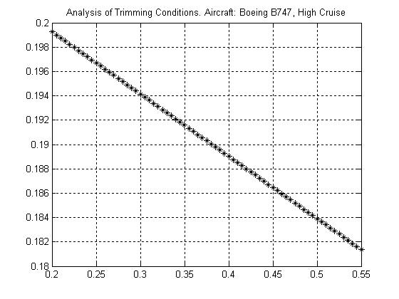
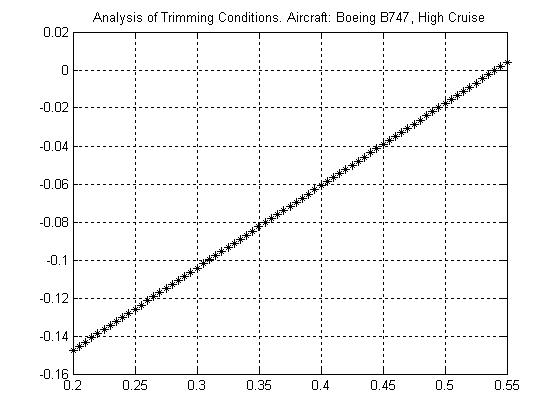
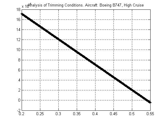
Problem 6.2

Consider the aerodynamic data for the McDonnell F-4 aircraft at high subsonic cruise conditions (Appendix B, Aircraft #10). This aircraft features an all moving horizontal tail (stabilators) for both maneuvering and trimming. Evaluate the following trimming characteristics:

Solution of Problem 6.2

From the data in Appendix B, Aircraft #10, we have the following:

Using the air density relationship from the Standard Atmospheric Model:

Therefore,

Given the following values for the longitudinal aerodynamic stability and control derivatives:

Next, evaluate 1 using:

The gradient

Also, the gradient

is evaluated using:

which is positive, as expected.

From the aerodynamic data in Appendix B the Static Margin for this aircraft at this configuration can be calculated using:

Starting from the reference center of gravity

An interested reader is also referred to chapter III for a validation of the above result.

Next, the moment arm associated with the horizontal tail can be calculated using: 0.58

The small size of this important geometric parameter is typical for a fighter aircraft.

The above leads, therefore, to: 1.451.450.291.74 H ACCG

Thus, the gradient

A plot of

can be evaluated using:

0.4(1.74) 1.5(1.74)1.5(0.397)

for a range of CGx locations is shown below:

Problem 6.3

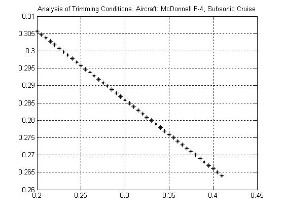
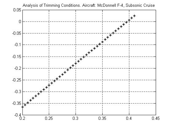
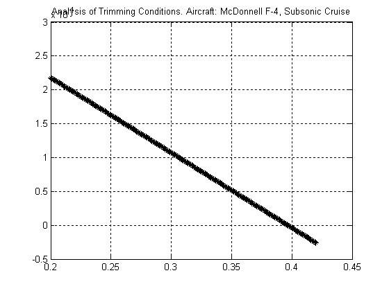
Consider a generic general aviation aircraft with the trim diagram shown below.

TrimDiagramforaGeneralAviationAircraft 0.3

Figure P6.3.1 – Trim Diagram for a Generic General Aviation Aircraft

The aircraft features stabilators   Hi for trimming purposes. Find the following:

- the aircraft aerodynamic center ACx ;

- the stabilator deflection required for trimming the aircraft at 1 5   with 0.42 CGx  ;

- the angle of attack required for trimming the aircraft with 4 Hi  and 0.25 CGx  ;

- the value of 0Lc and assessment on whether the aircraft can be trimmed with 10 LLcc  .

Solution of Problem 6.3

The aircraft aerodynamic center ACx is the ‘last’ position of the aircraft center of gravity at which the aircraft can be trimmed. Therefore, by definition, the aircraft will exhibit neutral longitudinal stability when CGACxx  ACx is found using information extracted from the AB segment of the trim diagram. Without any loss of generality, for simplicity purposes consider a point on the segment AB with 1 Lc  ; this point is associated with

0.18 m c  . Therefore, starting from 0.3 REFCGx  , ACx will be the point with a   SM  given by:

Note that any other point could have been considered on the segment AB leading to the same results. Thus, as shown below, ACx can be found as:

TrimDiagramforaGeneralAviationAircraft

Figure P6.3.2 – Calculation of ACx from the Trim Diagram

The stabilator deflection required for trimming the aircraft at 1 5   with 0.42 CGx  can be calculated as in the following. First, the segment AD associated with the center of gravity located at 0.42 CGx  can be found by ‘imposing’ a   0.12 SM  associated with 0.12 m c  and 1 Lc  , without any loss of generality. Next, the intersection between the segment AD and the line associated 1 5   is found and identified as point E. Next, a line which is parallel to the different stabilator deflection is found with the property that it intersects the above point E. This line is associated with a deflection of 1 3.5 Hi  . The above process is shown below.

TrimDiagramforaGeneralAviationAircraft

Figure P6.3.3 – Stabilator deflection required for trimming the aircraft at 1 5   with 0.42 CGx 

The angle of attack required for trimming the aircraft with 4 Hi  and 0.25 CGx  can be found as in the following. First, the segment AD associated with the center of gravity located at 0.25 CGx  can be found by ‘imposing’ a   0.05 SM  associated with 0.05 m c  and 1 Lc  , without any loss of generality. Next, the intersection between the segment AD and the line associated 4 Hi  is found and identified as point E. Next, a line which is parallel to the different angles of attack is found with the property that it intersects the above point E. This line is associated with a deflection of 6.5  . The above process is shown below.

TrimDiagramforaGeneralAviationAircraft

Figure P6.3.4 – Angle of attack required for trimming the aircraft with 4 Hi  and 0.25 CGx  The value of 0Lc can be found as in the following. By definition

0 EH LL i cc   ; therefore, since 0 E  , by intersecting the lines 0 Hi  and 0   we have point D indicating 0 0.05 Lc  . Since point ‘D’ is outside the trimming diagram it is clear that the aircraft can not be trimmed at those conditions. The above process is shown below.

TrimDiagramforaGeneralAviationAircraft

Figure P6.3.5 – Value of 0Lc

0.35

Problem 6.4

Consider a generic commercial aviation jetliner with the trim diagram shown below.

TrimDiagramforaCommercialAviationJetliner

Figure P6.4.1 – Trim Diagram for a Generic Commercial Aviation Jetliner

The aircraft features stabilators   Hi for trimming purposes. Find the following:

- the aircraft aerodynamic center ACx ;

- the stabilator deflection required for trimming the aircraft at 1 3   with 0.44 CGx  ;

- the angle of attack required for trimming the aircraft with 5 Hi  and 0.3 CGx  ;

- the value of 0Lc and assessment on whether the aircraft can be trimmed with 10 LLcc  .

Solution of Problem 6.4

The aircraft aerodynamic center ACx is the ‘last’ position of the aircraft center of gravity at which the aircraft can be trimmed. Therefore, by definition, the aircraft will exhibit neutral longitudinal stability when CGACxx  . ACx is found using information extracted from the AB segment of the trim diagram. Without any loss of generality, for simplicity purposes consider a point on the segment AB with 1 Lc  ; this point is associated with

0.2 m c  . Therefore, starting from 0.35 REFCGx  , ACx will be the point with a   SM  given by:

Note that any other point could have been considered on the segment AB leading to the same results. Thus, as shown below, ACx can be found as:

TrimDiagramforaCommercialAviationJetliner

Figure P6.4.2 – Calculation of ACx from the Trim Diagram

The stabilator deflection required for trimming the aircraft at 1 3   with 0.44 CGx  can be calculated as in the following. First, the segment AD associated with the center of gravity located at 0.44 CGx  can be found by ‘imposing’ a

 0.09 SM  associated with 0.09 m c  and 1 Lc  , without any loss of generality. Next, the intersection between the segment AD and the line associated 1 3   is found and identified as point E. Next, a line which is parallel to the different stabilator deflection is found with the property that it intersects the above point E. This line is associated with a deflection of 1 6 Hi  . The above process is shown below.

TrimDiagramforaCommercialAviationJetliner

Figure P6.4.3 – Stabilator deflection required for trimming the aircraft at 1 3   with 0.44 CGx 

The angle of attack required for trimming the aircraft with 5 Hi  and 0.3 CGx  can be found as in the following. First, the segment AD associated with the center of gravity located at 0.3 CGx  can be found by ‘imposing’ a   0.05 SM  associated with 0.05 m c  and 1 Lc  , without any loss of generality. Next, the intersection between the segment AD and the line associated 5 Hi  is found and identified as point E. Next, a line which is parallel to the different angles of attack is found with the property that it intersects the above point E. This line is associated with a deflection of 7  . The above process is shown below.

TrimDiagramforaCommercialAviationJetliner

Figure P6.4.4 – Angle of attack required for trimming the aircraft with 5 Hi  and 0.3 CGx  The value of 0Lc can be found as in the following. By definition

 ; therefore, since 0 E  , by intersecting the lines 0 Hi  and 0   we have point D indicating 0 0.13 Lc  . Since point ‘D’ is outside the trimming diagram it is clear that the aircraft can not be trimmed at those conditions. The above process is shown below.

TrimDiagramforaCommercialAviationJetliner

Figure P6.4.5 – Value of 0Lc

Problem 6.5

Consider an ‘engine-out’ condition for the Cessna 310 twin-engine aircraft (Appendix B, Aircraft #2). Describe the solution for new steady state conditions with an engine failure (right engine) occurring at approach conditions (see Appendix B) assuming:

Solution of Problem 6.5

Starting from the following aerodynamic and propulsive data of the Cessna 310 (Appendix B, Aircraft #2):

0.1683,0.0676,0.1152 0.0965,0.172,0.0192

Starting from the initial trimming conditions:

Assuming the failure of the right engine, assuming a negligible ‘toe-in’ angle and 1 0

, we will have a positive thrust-induced yawing moment given by:

Using the modeling described in this chapter, the following sequence of compensating actions can be taken by the pilot following the detection and the identification of the failure on the right engine:

Step #1 – Aileron compensating deflection 1A EO  to overcome the rolling moment associated with the engine failure:

The above value implies that due to the low dynamic pressure during the approach the engine-out condition is fairly simple to control from a directional point of view. Due to the low value of 1

, a secondary compensation for the ailerons will likely not be necessary. In fact, numerically we would have:

It is important to verify that the airspeed during approach ( 1PV =137.9 ft/sec) is above the ‘Minimum Control’ airspeed provided by:

At approach we can approximate: 33 0 2.3710/slugft 

Assuming a 25 for 1 MAX R EO  ,we would have:

which is substantially lower than 1PV =137.9 ft/sec.

From the above analysis it appears that a pilot should be able to handle the ‘engine-out’ condition without significant saturation problems on the lateral directional control surfaces. Since the aircraft is at approach and since the required compensating deflection for the rudder is quite small, it would not be recommended in this case to command a small bank angle into the operational engine. However, it would be recommended for the pilot to reduce 1 EO  with an additional compensating rudder deflection for a desirable alignment of the aircraft during the descent phase.

Problem 6.6

Consider the data for the Cessna 620 four-engine aircraft (Appendix B, Aircraft #5).

Describe the solutions for new steady state conditions with:

Scenario #1 - an engine failure for engine #1 engine on the right side, occurring at approach conditions (see Appendix B) assuming:

1 0.27 2 T b y 

Scenario #2 - simultaneous failures for an engine #1 and engine #2 on the right side, occurring at approach conditions (see Appendix B) assuming: 120.27,0.6

Solution of Problem 6.6

Scenario #1

Starting from the following aerodynamic and propulsive data of the Cessna 620 (Appendix B, Aircraft #5):

Starting from the initial trimming conditions:

For Scenario #1, assuming 1 0 TL  , we will have a positive thrust-induced yawing moment given by: 1111 11 0.273.070.58 422TT b NTyTlbsft

Using the modeling described in this Chapter, the following sequence of compensating actions can be taken by the pilot following the detection and the identification of the failure on the right engine:

Step #1 – Aileron compensating deflection 1A EO  to overcome the rolling moment associated with the engine failure:

The low magnitude of the above value implies that due to the low dynamic pressure during the approach the engine-out condition is fairly simple to control from a directional point of view.

Due to the low value of 1R EO  , a secondary compensation for the ailerons will likely not be necessary. In fact, numerically we would have:

It is important to verify that the airspeed during approach ( 1PV =189.2 ft/sec) is above the ‘Minimum Control’ airspeed provided by:

At approach we can approximate: 33 0 2.3710/slugft

Assuming a 25  for 1 MAX R EO  ,we would have:

which is substantially lower than 1PV =189.2 ft/sec.

From the above analysis it appears that a pilot should be able to handle the ‘engine-out’ condition without any problem Since the aircraft is at approach and since the required compensating deflection for the rudder is quite small, it would not be recommended in this case to command a small bank angle into the operational engine.

Scenario #2

Starting from the above aerodynamic and propulsive data of the Cessna 620 (Appendix

B, Aircraft #5), for Scenario #2, assuming 1 0 TL  , we will have a positive thrust-induced yawing moment given by:

Step #1 – Aileron compensating deflection 1A EO  to overcome the rolling moment associated with the engine failure:

Step #2 – Rudder compensating deflection

to regain equilibrium around the yawing axis:

Even for the case of simultaneous failure for 2 engines, the low magnitude of the above value implies that due to the low dynamic pressure during the approach the engines-out condition is fairly simple to control from a directional point of view.

Due to the low value of 1R EO  , a secondary compensation for the ailerons will likely not be necessary. In fact, numerically we would have:

It is important to verify that the airspeed during approach ( 1PV =189.2 ft/sec) is above the ‘Minimum Control’ airspeed provided by:

At approach we can approximate: 33 0 2.3710/slugft

Assuming a 25  for 1

EO  ,we would have:

which is, again, substantially lower than 1PV =189.2 ft/sec.

From the above analysis it appears that a pilot should be able to handle the 2 ‘same side engines-out’ condition without any problem. Since the aircraft is at approach and since the required compensating deflection for the rudder is quite small, it would not be recommended in this case to command a small bank angle into the operational engine.

Problem 7.1

Problems for Chapter VII

Consider the SIAI Marchetti S211 aircraft at cruise #1 flight conditions (Appendix B, Aircraft #8). From the available data first find the „full‟ longitudinal characteristic equations, the associated roots, and evaluate the short period and phugoid characteristics. Next, find the characteristic equations associated with the short period and phugoid approximations. For both dynamic modes evaluate the error differences in terms of natural frequency and damping between the „full‟ and the „approximated‟ characteristic equations.

Solution of Problem 7.1

Determination of the „Full‟ longitudinal characteristic equation Tables P7.1.1 and P7.1.2 show the aircraft data.

Flight Conditions

Table P7.1.1 - Flight conditions, geometry, and mass data for the SIAI Marchetti S211 Aircraft

Steady State Coefficients

Longitudinal Coefficients and Stability Derivatives

Table P7.1.2 - Longitudinal aerodynamic data for the SIAI Marchetti S211 aircraft

Next, the numerical values of the longitudinal dimensional stability and control derivatives are calculated

32cos(0)0.13497.270601189.571300

32sin(0)006.24730.03320.00217.2706031.387

Using the Matlab, the roots associated with the Short Period and the Phugoid modes are:

1,2 2.7853 1.9882 SP rootsi  1,2 0.0171 0.0638 Ph rootsi  leading to:

22 2.78531.98823.4221sec SP rad

2.7853 cos0.8139 3.4221 SPSP

 0.0171 cos0.2587 0.0661 PhPh 

22 0.01710.06380.0661sec Ph rad

Figure P7.1.1 shows the above roots in the s-domain.

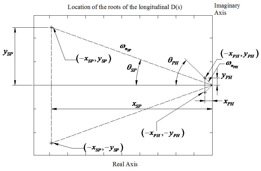
Figure P7.1.2 - Location of the roots of the longitudinal D(s)

Short Period Approximation

The

Phugoid Approximation

Error Differences

Table P7.1.3 and Table P7.1.4 show the errors in the natural frequency and damping between the “full” and the “approximated” characteristic equations.

Short Period Approximation

“Full”

Table P7.1.3 - Error analysis for the Short Period characteristics “Full” Phugoid Approximation

Table P7.1.4 - Error analysis for the Phugoid characteristics

Problem 7.2

Consider the Mc Donnell F-4 aircraft at subsonic cruise flight conditions (Appendix B, Aircraft #10). From the available data first find the „full‟ longitudinal characteristic equations, the associated roots, and evaluate the short period and phugoid characteristics. Next, find the characteristic equations associated with the short period and phugoid approximations. For both dynamic modes evaluate the error differences in terms of natural frequency and damping between the „full‟ and the „approximated‟ characteristic equations.

Solution of Problem 7.2

„Full‟ longitudinal characteristic equations

Tables P2.1 and P2.2 show the aircraft data.

Flight Conditions

1 2.6 deg = 0.045rad q 283.2 lb/ft2

1PV 876 ft/s

1 0 deg=0 rad

1 2.6 deg = 0.045 rad Geometry S 530 ft2 c 16 ft Mass Data

Table P7.2.1 - Flight conditions, geometry and mass data for the Mc Donnell F-4 Aircraft

Steady State Coefficients

Longitudinal Coefficients and Stability Derivatives

Table P7.2.2 - Longitudinal coefficients and stability derivatives for the Mc Donnell F-4 aircraft

Next, the longitudinal dimensional stability derivatives are calculated using:

0.01220.00060.48468760.9673465.5

0.23338762.02450.4846465.50.11114.9262

4.92620.002602.02458760.11114.92620.4846 0.01220.00067.86102.02458760.4846465.54.9555

32cos(0.045)0.11117.8610465.50.00260

32sin(0.045)0.002604.92620.01220.00067.861011.279

leading to:

432

1()876.971105.671094.955511.279 Dsssss 

Using Matalb, the roots of the Short Period and Phugoid dynamic modes are given by:

leading

It is clear that the Phugoid mode has degenerated into 2 real roots, of which one is unstable. This analytical condition is typically associated with the aerodynamic transonic condition known as „Tuck‟, which is due to a sudden and drastic shift in the aircraft aerodynamic center for a small Mach increment. Figure P7.2.1 shows the location of the roots in the s-domain

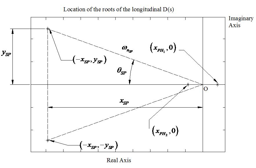
Figure P7.2.1-Location of the roots of the longitudinal D(s)

Short Period Approximation

The characteristic equation for the short period approximation is,

Inserting the values of the terms,

Error Differences

Table P7.2.3 shows the analysis of the error using the Short Period approximation.

Table P7.2.3 - Error analysis for the Short Period characteristics

A similar error analysis for the Phugoid mode is not possible since the Phugoid mode has degenerated for this aircraft at this specific flight condition.

Problem 7.3

Consider the Beech 99 aircraft at high cruise flight conditions (Appendix B, Aircraft #3). From the available data first find the „full‟ longitudinal characteristic equations, the associated roots, and evaluate the short period and phugoid characteristics. Next, find the characteristic equations associated with the short period and phugoid approximations. For both dynamic modes evaluate the error differences in terms of natural frequency and damping between the „full‟ and the „approximated‟ characteristic equations.

Solution of Problem 7.3

„Full‟ longitudinal characteristic equations Tables P7.3.1 and P7.3.2 show the aircraft data.

Table P7.3.1. Flight conditions, geometry and mass data for the Beech 99 Aircraft

Steady State Coefficients

Longitudinal Coefficients and Stability Derivatives

Table P7.3.2. Longitudinal coefficients and stability derivatives for the Beech 99 Aircraft

Next the longitudinal dimensional stability derivatives are evaluated using:

0.0138021.776906.10884502.8293575.4153.96

32cos(0.019)0.146721.77690575.400 32sin(0.019)0018.27430.0138021.77690102

leading

Using Matlab, the roots of the „full‟ longitudinal characteristic equation are given by: 1,2 2.4242 4.3729 SP rootsi  1,2 0.0059 0.0948 Ph rootsi  leading to:

22 2.42424.37295sec SP rad   2.4242 cos0.4848 5 SPSP 

22 0.00590.09480.09498sec PH rad   0.0059 cos0.06212 0.09498 PhPh 

Figure P7.3.1 shows the location of the roots on the s-domain.

Figure P7.3.1-Location of the roots of the longitudinal D(s)

Short Period Approximation

The

Phugoid Approximation The

Therefore, the associated values of the phugoid characteristics are given by: 0.01040.102sec

Error Differences

Table P7.3.3 and Table P7.3.4 show the analysis of the errors in the natural frequency and in the damping ration between the “full” and the “approximated” characteristic equations.

Table P7.3.3 - Error differences for the Short Period approximation

Table P7.3.4 - Error differences for the Phugoid approximation

Problem 7.4

Consider an aircraft static model mounted on a scale in a wind tunnel. The interface between the scale and the model is such that the model is only able to rotate around its S YY  stability axis. Since the model is not able to perform neither a climb or a descent, for all practical purposes we would have ,   . Therefore, the single degree of freedom equation describing the dynamic of the system is given by:

Derive relationships for the short period natural frequency and damping from the given equation and compare them with the same relationships derived using the short period approximation.

Solution of Problem 7.4

Starting from the previous equation describing the dynamics of the single DOF system:

The equation can be rewritten as:

Applying Laplace Transformation (assuming zero initial conditions),

Solving for

Equating the denominator with the generic form of the characteristic equation for the short period approximation:

as opposed to:

Both expressions differ due to the missing term Z  for the aircraft static model. Recall:

Since the static model can not climb or descend (it is restrained or fixed in the Zdirection) the effect of the variation in the angle of attack does not have effect in the total lift force over the model.

Problem 7.5

Consider again the Mc Donnell F-4 aircraft at subsonic cruise flight conditions (Appendix B, Aircraft #10). From the available dimensionless aerodynamic derivatives, geometric data, inertial data, and flight conditions at subsonic cruise conditions, develop a Matlab code performing a complete analysis of the aircraft lateral directional dynamics. Clearly identify the roots and the characteristics associated with the dutch roll, the rolling, and the spiral modes. Plot the lateral directional responses of the aircraft following short doublets on ailerons and rudder. Be careful in selecting the magnitude of the maneuvers such that the aircraft response does not go over the limitations associated with the small perturbation assumptions.

Solution of Problem 5

Data and Dimensional Stability Derivatives

Tables P7.5.1, P7.5.2, and P7.5.3 show the aircraft data. Table P7.5.4 shows the values of the dimensional lateral-directional stability and control derivatives. Flight Conditions

Table P7.5.1. Flight conditions, geometry and mass data for the Mc Donnell F-4 Aircraft

Lateral-Directional Stability Derivatives

Derivative Value

lc  -0.08

plc -0.240

rlc 0.07 y c  -0.68 py c 0 ry c 0 n c  0.125 Tn c  0 pn c

Lateral-Directional Control Derivatives

R n c  -0.066

Table P7.5.2. Lateral/directional aerodynamic coefficients for the Mc Donnell F-4 Aircraft

Table P7.5.3. Moments and products of inertia with respect to the stability axes Derivative Value

Table P7.5.4. Dimensional lateral/directional stability and control derivatives for the F-4 Aircraft

Transfer Functions

The lateral directional dynamics is excited by the deflection of (at least) two control surfaces, that is aileron and rudder, leading to the following set of 6 transfer functions: 432 5432 () 1.965217638.276.81 ()873.713815302677587.58 A sssss ssssss

5432 ()8540295743880 ()873.713815302677587.58 A ssss ssssss

5432 ()219.9358.945.051595 ()873.713815302677587.58 A ssss ssssss

5432 ()11.672446305520.45 ()873.713815302677587.58 R sssss ssssss

()150864038350 ()873.713815302677587.58 R ssss ssssss

()24293163204.51398 ()873.713815302677587.58 R ssss ssssss

Analysis of the Dynamic Stability

The lateral-directional characteristic equation is

Using the above coefficients the lateral-directional dynamic stability analysis is performed and presented in Table P7.5.5 The application of the Routh-Hurwitz stability criteria predicts the stability of the lateral directional dynamics.

Table P7.5.5. Lateral-directional dynamic stability conditions

Roots of the Lateral-Directional Characteristic Equation

Using Matlab, the roots of the lateral-directional characteristic equation 2()Ds are given by:

Discarding the „trivial‟ root at „0‟, the above roots are associated with the following dynamic modes:

1,2

Figure P7.5.1 shows the location of the roots

McDonnellF-4Lateral-DirectionalDynamics(Mach=0.9,h=35000ft).D2(s)roots

Figure P7.5.1 – Location of the roots of the lateral-directional characteristic equation

Dynamic Simulation

Figures P7.5.2 through Figure P7.5.9 show the ,  ,and time histories following short doublets for the aileron and rudder generated using a Matlab code based on the use of the powerful “LSIM” command.

McDonnellF-4Lateral-DirectionalDynamics(Mach=0.9,h=35000ft)

Figure P7.5.2 - Aileron doublet maneuver for the F4 aircraft

McDonnellF-4Lateral-DirectionalDynamics. AileronManeuver.(Mach=0.9,h=35000ft)

P7.5.3 - Beta time history following aileron maneuver for the F4 aircraft

McDonnellF-4Lateral-DirectionalDynamics.AileronManeuver.(Mach=0.9,h=35000ft)

Figure P7.5.4 - Phi time history following aileron maneuver for the F4 aircraft

Figure

McDonnellF-4Lateral-DirectionalDynamics.AileronManeuver.(Mach=0.9,h=35000ft)

P7.5.5 - Psi time history following aileron maneuver for the F4 aircraft

McDonnellF-4Lateral-DirectionalDynamics.(Mach=0.9,h=35000ft)

P7.5.6 - Rudder doublet maneuver for the F4 aircraft

Figure

McDonnellF-4Lateral-DirectionalDynamics.RudderManeuver.(Mach=0.9,h=35000ft)

P7.5.7 - Beta time history following rudder maneuver for the F4 aircraft

McDonnellF-4Lateral-DirectionalDynamics.RudderManeuver.(Mach=0.9,h=35000ft)

P7.5.8 - Phi time history following rudder maneuver for the F4 aircraft

Figure

McDonnellF-4Lateral-DirectionalDynamics.RudderManeuver.(Mach=0.9,h=35000ft)

Figure P7.5.9 - Psi time history following rudder maneuver for the F4 aircraft

Problem 7.6

Consider the Cessna T37 aircraft at cruise flight conditions (Appendix B, Aircraft #2). Using the „empirical‟ modeling for the key longitudinal stability and control derivatives described in Chapter III, along with the relationships for the dimensional stability derivatives in Table 7.1, perform a short period sensitivity analysis using the available dimensionless aerodynamic derivatives, geometric data, inertial data, and flight conditions at cruise conditions. Specifically, focus on the dependencies of the short period characteristics with the following parameters: ,, H CGYY S xI S

Solution of Problem 7.6

The „Short Period‟ approximation provides the following relationships for the natural frequency and the damping coefficient:

Thus, the dimensional stability derivatives affecting SPn  and SP are:

The dimensionless derivatives associated with the above dimensional derivatives are:

in addition to the value of the drag coefficient at trim conditions 1Dc . It can be approximated that 1 DLcc   .

The geometric parameters HS S

, MAC were found using the measurements extracted from Figure P7.6.1.

Figure P7.6.1 - MODIFIED 3D view of Cessna T37 Aircraft (Source: http://www.aviastar.org/index2.html)

Using HS S

, MAC , the geometric parameter

H ACCGxx was evaluated using the distances in Figure P7.6.2:

Figure P7.6.2-Wing-Horizontal Tail Geometric Distances

Therefore, the following geometric parameters were extracted and considered to be the values associated at „Design Condition‟: 0.261 HS S

2.894 H ACCGxx

Table P7.6.1 summarizes the values of the different geometric and inertial parameters along with the aerodynamic coefficients used for the calculation of the dimensional stability derivatives.

Design Condition Values

Table P7.6.1 - Values of the parameters at the design condition for the Cessna T-37

Variation with respect to

Considering the „Design Condition‟ as the initial conditions, all the dimensionless stability derivatives have a linear dependency with H

; therefore, they can be calculated using a 1st order Taylor expansion starting from the „initial condition‟ being the „design condition‟. Therefore, we would have:

using the geometric parameters showing in Figure P6.1 along with the modeling procedures outlined in Chapter III.

it is possible to evaluate the relationships for the associated dimensional derivatives:

leading ultimately to the relationships:

The

S P

CessnaT37@cruise. Short PeriodSensitivity Analysis. Parameter:S/SH

P7.6.3 - Variation of SPn  with HS S

for the Cessna T-37

CessnaT37@Cruise. Short PeriodSensitivity Analysis. Parameter:S/SH

P7.6.4 - Variation of SP with HS S

for the

Figure

Cessna T-37

Variation with respect to CGx

A similar analysis in terms of CGx is slightly more complicated due to the fact that the stability derivatives m c  and qm c are function of 2 CGx . Therefore, a 2nd order Taylor series expansion was used to express the relationships

and

 qq mmCG ccx  . On the other side Lc  does not depend on CGx while mc  is a linear function of CGx ; therefore, a 1st order Taylor expansion would be appropriate for

A similar process is used for expressing the relationship

The associated trends are shown in Figures P7.6.5 and P7.6.6.

CessnaT37@cruise. Short PeriodSensitivity Analysis. Parameter:XCG(% ofMAC)

P7.6.5 -Variation of SPn  with CGx for the

CessnaT37@Cruise. Short PeriodSensitivity Analysis. Parameter:XCG(% ofMAC)

P7.6.6 -Variation of SP with CGx for the

Figure

Cessna T-37

Figure

Cessna T-37

Variation with respect to yy I

The value of yy I only affects the value of the dimensional stability derivatives; therefore, an analysis can be obtained directly from ,, YYYYYY q III MMM  leading to the results in Figures P6.7 and P6.8.

CessnaT37@cruise.ShortPeriodSensitivityAnalysis.Parameter:IYY

IYY [slugft2]

Figure P7.6.7 - Variation of SPn  with yy I for the Cessna T-37

CessnaT37@Cruise.ShortPeriodSensitivityAnalysis.Parameter:IYY

IYY [slugft2]

Figure P7.6.8 - Variation of SP with yy I for the Cessna T-37

Problem 7.7

Consider again the Cessna T37 aircraft at cruise flight conditions (Appendix B, Aircraft #2). Using the relationships for the dimensional stability derivatives in Table 7.3, perform a lateral directional sensitivity analysis using the available dimensionless aerodynamic derivatives, geometric data, inertial data, and flight conditions at cruise conditions. Specifically, focus on the dependencies of the dutch roll, rolling, and spiral characteristics with the following parameters:

, xxzz II

Solution of Problem 7.7

As described in Chapter VII, there are no direct explicit relationships for the dutch roll, and spiral characteristics as a function of the dimensionless stability derivatives. The exception is given by the rolling mode, which is a single degree-of-freedom mode known to have a clear and simple relationship with one aerodynamic derivative ( plc ) and one moment of inertia ( xx I ). Therefore, for a detailed sensitivity analysis of the lateral directional dynamics it is necessary to determine the variation of the roots of the characteristic equation for a range of values of a given parameter (dimensionless derivative or moment of inertia).

The following are the plots of the variation the Dutch roll, rolling, and spiral characteristics with respect to the parameters ,,,, pr lnlny ccccc  , , xxzz II . They were obtained using a Matlab code that evaluates the roots of the characteristic equation for several values of a single parameter (either a dimensionless derivative or a moment of inertia) with an arbitrarily set range of variation of ±10% from the design condition. For example, given the design condition of lc  value of -0.0944, the associated range is from -0.10384 to -0.08496 (see Figure P7.7.1).

CessnaT37@cruise.DutchRollSensitivityAnalysis.Parameter:cbeta

CessnaT37@cruise.SpiralSensitivityAnalysis.Parameter:cbea

P7.7.1 - Variation of DR with lc 

CessnaT37@Cruise.DutchRollSensitivityAnalysis.Parameter:clbeta

Figure P7.7.2 - Variation of DR with

CessnaT37@cruise.RollingSensitivityAnalysis.Parameter:clbeta

Figure P7.7.3 - Variation of RT with

P7.7.4 - Variation of ST with lc 

CessnaT37@cruise.DutchRollSensitivityAnalysis.Parameter:cnbea

Figure P7.7.5 - Variation of DR with n c

CessnaT37@Cruise.DutchRollSensitivityAnalysis.Parameter:cnbeta

Figure P7.7.6 - Variation of DR with n c 

Figure

TR [sec]

CessnaT37@cruise.RollingSensitivityAnalysis.Parameter:cnbeta

CessnaT37@Cruise.DutchRollSensitivityAnalysis.Parameter:clp

Figure P7.7.7 -Variation of RT with n c 

CessnaT37@cruise.SpiralSensitivityAnalysis.Parameter:cnbeta

Figure P7.7.10 - Variation of DR with p lc

CessnaT37@cruise.RollingSensitivityAnalysis.Parameter:cp

Figure P7.7.8 - Variation of ST with n c 

CessnaT37@cruise.DutchRollSensitivityAnalysis.Parameter:clp

Figure P7.7.11 - Variation of RT with p lc

CessnaT37@cruise.SpiralSensitivityAnalysis.Parameter:cp

Figure P7.7.9 - Variation of DR with p lc

Figure P7.7.12 - Variation of ST with p lc

CessnaT37@cruise.DutchRollSensitivityAnalysis.Parameter:cnr

CessnaT37@cruise.SpiralSensitivityAnalysis.Parameter:cnr

Figure P7.7.13 - Variation of DR with rn c

CessnaT37@Cruise.DutchRollSensitivityAnalysis.Parameter:cnr

Figure P7.7.16 - Variation of ST with rn c

CessnaT37@cruise.DutchRollSensitivityAnalysis.Parameter:cybeta

Figure P7.7.14 - Variation of DR with rn c

CessnaT37@cruise.RollingSensitivityAnalysis.Parameter:cnr

Figure P7.7.17 - Variation of DR with y c 

CessnaT37@Cruise.DutchRollSensitivityAnalysis.Parameter:cybeta

Figure P7.7.15 - Variation of RT with rn c

Figure P7.7.18 - Variation of DR with y c 

TR [sec]

CessnaT37@cruise.RollingSensitivityAnalysis.Parameter:cybeta

CessnaT37@Cruise.DutchRollSensitivityAnalysis.Parameter:Ixx

Figure P7.7.19 - Variation of RT with y c 

CessnaT37@cruise.SpiralSensitivityAnalysis.Parameter:cybeta

P7.7.22 - Variation of DR with xx I

CessnaT37@cruise.RollingSensitivityAnalysis.Parameter:Ixx

Figure P7.7.20 - Variation of ST with y c 

CessnaT37@cruise.DutchRollSensitivityAnalysis.Parameter:Ixx

Figure P7.7.23 - Variation of RT with xx I

CessnaT37@cruise.SpiralSensitivityAnalysis.Parameter:Ixx

Figure P7.7.21 - Variation of DR with xx I

Figure P7.7.24 - Variation of ST with xx I

Figure

CessnaT37@cruise.DutchRollSensitivityAnalysis.Parameter:Izz

CessnaT37@cruise.RollingSensitivityAnalysis.Parameter:Izz

Figure P7.7.25 - Variation of DR with zz I

CessnaT37@Cruise.DutchRollSensitivityAnalysis.Parameter:Izz

Figure P7.7.27 - Variation of RT with zz I

CessnaT37@cruise.SpiralSensitivityAnalysis.Parameter:Izz

Figure P7.7.26 - Variation of DR with zz I

Figure P7.7.28 - Variation of ST with zz I

Problems for Chapter VIII

Problem 8.1

Consider a linear dynamic system described by the following Differential Equation (DE) with constant coefficients: ()5()7()3()() ytytytytut 

Find the state variable model associated with this system. Verify that the eigenvalues of the state matrix A are coincident with the roots of the characteristic equation of the above system.

Solution of Problem 8.1.

The system is a 3rd order system with 1 input and 1 output  3,1,1nml . A suitable selection of state variables is given by: 1 2 2 33 2 ()() () ()() () ()()()() xtyt dyt xtyt dt dyt xtytxtyt dt

Using the system DE equation, 3()()5()7()3()() xtytytytytut 

Rewriting the above equations using the state variables will lead to the following: 1 12 23 3321 ()() ()() ()() ()5()7()3()() xtyt xtxt xtxt xtxtxtxtut

Thus, the state variable model in a matrix format is given by:

11 22 33 ()010()0 ()001()0() ()375()1 xtxt xtxtut xtxt

The characteristic equation is given by:

with roots :

The eigenvalues of the system matrix are,

The SV output equation is given by,

Problem 8.2

Consider a linear dynamic system described by the following set of Differential Equations (DEs) with constant coefficients:

121 2122 ()5()() ()3()2()() ytytut ytytytut 

- Find the state variable model of the above system.

- The system is subjected to 2 inputs   12(),()utut and has two measurable outputs

  12(),()ytyt . Therefore, a transfer function-based modeling of the system will require the evaluation of a (2 x 2) matrix of transfer functions. Find the matrix of transfer functions under the following conditions:

- Derivation directly from the DEs

- Derivation from the state variable model.

Solution of Problem 8.2

State Variable Model

The system is a 2nd order system with 2 inputs and 2 outputs

suitable selection of state variables is given by:

Using the system DE equation,

2122 ()5()() ()3()2()() xtxtut xtxtxtut

Rearranging:

2122 ()5()() ()3()2()()

Thus, the SV state equation is given by:

111 222 ()()() 0510 ()()() 3201 xtxtut xtxtut

The SV output equation is given by,

Derivation of Transfer Function (TF) matrix DIRECTLY from the DEs

Following the application of the Laplace transformation to the above system we have:

leading to the following matrix format: 11 22 ()() 5 ()() 3(2) YsUs s YsUs s

By invoking the „superimposition of effect‟ property of linear systems, we can solve the above system first considering 22 ()0()0utUs and, next, considering 11 ()0()0utUs . The goal is to find all the () ij Gs transfer functions in the relationship:

Therefore, consider the system:

Using Cramer‟s rule we have:

0(2) (2)() () 5 (2)3(5) 3(2) (2)()() (2) () 215()215 Us s sUs Ys s ss s sUsYs s Gs ssUsss

11 11 22

Next, consider the system:

Using Cramer‟s rule again we have:

Thus, the (2 x 2) matrix of transfer functions is given by:

Derivation of Transfer Function (TF) matrix through the State Variable (SV) model

Starting from:

Once the matrices of the SV model are available, the matrix of the transfer functions ()Gs can be derived using the relationship:

Note that in this specific case, the D matrix is a zero matrix. A key step is the evaluation

The inverse of the matrix is

Problem 8.3

Consider a linear dynamic system described by the following set of Differential Equations (DEs) with constant coefficients: 121 22122 ()7()3() ()3()2()5()4() ytytut ytytytytut

- Find the state variable model of the above system.

- The system is subjected to 2 inputs   12(),()utut and has two measurable outputs

 

12(),()ytyt . Therefore, a transfer function-based modeling of the system will require the evaluation of a (2 x 2) matrix of transfer functions. Find the matrix of transfer functions under the following conditions:

- Derivation directly from the DEs

- Derivation from the state variable model.

Solution of Problem 8.3

State Variable Model

The system is a 2nd order system with 2 inputs and 2 outputs

nml . A suitable selection of state variables is given by: 11 22 322 32 ()() ()() ()()() ()() xtyt xtyt xtytxt xtyt

Using the system DE equation, 121 33122 ()7()3() ()3()2()5()4() xtxtut xtxtxtxtut

Rearranging, 121 23 31232 ()7()3() ()() ()2()5()3()4() xtxtut

Thus, the SV state equation is given by:

The SV output equation is given by:

Derivation of Transfer Function (TF) matrix DIRECTLY from the DEs

Following the application of the Laplace transformation to the above system we have:

leading to the following matrix format:

Therefore, consider the system:

Using Cramer‟s rule we have:

Using

Thus

Derivation of Transfer Function (TF) matrix through the State Variable (SV) model

Once the matrices of the SV model are available, the matrix of the transfer functions ()Gs can be derived using the relationship:

Note that in this specific case, the D matrix is a zero matrix.

A key step is the evaluation of

Using the “Adjoint/Transpose” approach for the evaluation of the inverse of the matrix, we have:

Problem 8.4

Consider the Learjet 24 aircraft at approach (Appendix B, Aircraft #6). Using the data provided in Appendix B, derive an “extended version” of longitudinal state variable (SV) model – shown below - featuring one additional input   Hi and one additional output

Verify that the eigenvalues of the state matrix LongA are coincident with the roots of the longitudinal characteristic equation provided in Appendix B (Aircraft #6).

Solution of Problem 8.4

Using the outlined procedure, for the selected aircraft at the selected flight condition we would have:

Longitudinal Dimensional Stability Derivatives

X_u: -0.058486 (ft/sec2)/(ft/sec)

X_alpha: 11.2631 (ft/sec2)/(rad)

X_de: 0 (ft/sec2)/(rad)

X_ih: 0 (ft/sec2)/(rad)

X_Tu: -0.010052 (ft/sec2)/(ft/sec)

Z_u: -0.37924 (ft/sec2)/(ft/sec)

Z_alpha: -102.8434 (ft/sec2)/(rad)

Z_alpha_dot: -0.63969 (ft/sec2)/(rad/sec)

Z_q: -1.6392 (ft/sec2)/(rad/sec)

Z_de: -7.7676 (ft/sec2)/(rad)

Z_ih: -16.5062 (ft/sec2)/(rad)

M_u: -0.00017279 (rad/sec2)/(ft/sec)

M_alpha: -1.9387 (rad/sec2)/(rad)

M_alpha_dot: -0.30238 (rad/sec2)/(rad/sec)

M_q: -0.81642 (rad/sec2)/(rad/sec)

M_de: -2.8786 (rad/sec2)/(rad)

M_ih: -6.1685 (rad/sec2)/(rad)

M_Tu: 0 (rad/sec2)/(ft/sec)

M_Talpha: 0 (rad/sec2)/(rad)

Primed Longitudinal Dimensional Stability Derivatives

Alpha-Dot Coefficients:

Z_u_prime: -0.0022225

Z_alpha_prime: -0.60269

Z_q_prime: 0.98665

Z_theta_prime: -0.016344

Z_de_prime: -0.045521

Z_ih_prime: -0.096731

U-Dot Coefficients:

X_u_prime: -0.068538

X_alpha_prime: 11.2631

X_theta_prime: -31.8782

X_q_prime: 0

X_ee_prime: 0

X_ih_prime: 0

Q-Dot Coefficients:

M_u_prime: 0.00049924

M_alpha_prime: -1.7564

M_theta_prime: 0.0049422

M_q_prime: -1.1148

M_de_prime: -2.8649

M_ih_prime: -6.1393

Double Primed Longitudinal Dimensional Stability Derivatives

a_z Coefficients:

Z_alpha_pprime: -105.2469

Z_u_pprime: -0.37782

Z_q_pprime: -2.2703

Z_theta_pprime: 0.010455

Z_de_pprime: -7.7385

Z_ih_pprime: -16.4443

State Equations

-0.068511.26310-31.8782

-0.0022-0.60270.9866-0.0163

0.0005-1.7564-1.11480.0049

-0.0455-0.0967

-2.8649-6.1393

Output Equations

The additional output   x a is found in a similar way as Za was found. A general expression for Xa is given by:

Using the 1st equation of the small perturbation Conservation of Linear Momentum Equations (CLMEs) expressed in the body axes:

Rewriting the above equation along the stability axes, since 1 0 S W  ,we would have :

 1 cos XXATmumgff  

Since   , we would have:

 11coscos XXATmumgmgff  

Thus, the aerodynamic and thrust along the stability axes can be expressed using:

 11coscos XXAT ffmumgmg

Therefore, an expression for Xa is given by:

From the previous modeling of the state variables, a relationship for u is given by: H uqEEiH uXuXXqXXXi  

Therefore: 11coscos H XuqEEiH aXuXXqXXXigg 

Grouping the terms with the same variables we would have:

Rearranging in a matrix format, the longitudinal „output equations‟ take on the form:

Problem 8.5

Consider the Learjet 24 aircraft at approach (Appendix B, Aircraft #6). Using the data provided in Appendix B, derive ONLY the state equations of the longitudinal state variable (SV) model shown below:

Next, consider as “baseline” the “nominal” values for the following dimensionless stability derivatives:

quLmmmm ccccc

Starting from the “nominal” value, for EACH of the above stability derivatives build a column vector where the value of the selected derivative (among the 8 derivatives above) varies from -20% to +20% with respect to the nominal value with increments of 1%.

- For EACH stability derivative plot the migration of the eigenvalues of LongA in the s-domain. Highlight the conditions where loss of dynamic stability occurs.

- Plot ,,,SPPh nSPnPh  versus. EACH stability derivative.

Solution of Problem 8.5

From Problem 8.4:

Figures P8.5.1, P8.5.3, P8.5.5, P8.5.7, and P8.5.9 show the eigenvalues migration for each stability derivative. It can de seen that the real parts of the eigenvalues are always positive; therefore, no loss of longitudinal dynamic stability occurs. Figures P8.5.2, P8.5.4, P8.5.6, P8.5.8, and P8.5.10 show the ,,,SPPh nSPnPh  variation with respect to each stability derivative.

EigenvaluesMigration. CLalpha variation.PhugoidEigenvalues

ofnominalCLalpha NominalCLalpha

Figure P8.5.1 - Eigenvalues Migration with Variation of Lc 

LongitudinalDynamics -Short Period

LongitudinalDynamics -Phugoid

LongitudinalDynamics -Short Period Nominal CLalpha

Figure P8.5.2 - ,,,SPPh nSPnPh

Eigenvalues Migration. Cmalpha variation.ShortPeriodEigenvalues

LongitudinalDynamics -Phugoid

CLalpha

with variations of Lc 

Eigenvalues Migration. Cmalpha variation.PhugoidEigenvalues

Figure P8.5.3 - Eigenvalues Migration with Variations of m c 

LongitudinalDynamics-ShortPeriod Nominal Cmalpha

LongitudinalDynamics-ShortPeriod

Nominal Cmalpha

LongitudinalDynamics-Phugoid Nominal Cmalpha

LongitudinalDynamics-Phugoid

Nominal Cmalpha

Figure P8.5.4 - ,,,SPPh nSPnPh

EigenvaluesMigration. Cmalphadot variation.ShortPeriodEigenvalues

with Variations of

EigenvaluesMigration. Cmalphadot variation.PhugoidEigenvalues

80%ofnominalCmalphadot

NominalCmalphadot

Figure P8.5.5 - Eigenvalues Migration with Variations of

LongitudinalDynamics -ShortPeriod

Nominal Cmalphadot

LongitudinalDynamics -Phugoid Nominal Cmalphadot

Damping Ratio

LongitudinalDynamics -ShortPeriod

Nominal Cmalphadot

LongitudinalDynamics -Phugoid

Nominal Cmalphadot

Figure P8.5.6 - ,,,SPPh nSPnPh

with Variations of m c

Eigenvalues Migration. C mq variation. Short PeriodEigenvalues

Eigenvalues Migration. C mq variation. PhugoidEigenvalues

80% ofnominalC mq NominalC mq

Figure P8.5.7 - Eigenvalues Migration with Variation of q m c

LongitudinalDynamics -ShortPeriod

LongitudinalDynamics -Phugoid

Figure P8.5.8. ,,,SPPh nSPnPh

Eigenvalues Migration. C mu variation.ShortPeriodEigenvalues

LongitudinalDynamics -Phugoid Nominal C mq

with Variations of q m c

Eigenvalues Migration. C mu variation.PhugoidEigenvalues

Figure P8.5.9 - Eigenvalues Migration with Variations of u m c

Short Period Natural Frequency

LongitudinalDynamics -Short Period Nominal C mu

Short Period Damping Ratio

LongitudinalDynamics -Phugoid

LongitudinalDynamics -Short Period

Nominal C mu

LongitudinalDynamics -Phugoid

Nominal C mu

P8.5.10 - ,,,SPPh nSPnPh

with Variations of u m c

Figure

Problem 8.6

Consider the McDonnell Douglas F-4 aircraft at subsonic conditions (Appendix B, Aircraft #10). Using the data provided in Appendix B, derive ONLY the state equations of the longitudinal state variable (SV) model shown below:

Next, consider as “baseline” the “nominal” values for the following dimensionless stability derivatives:

- For EACH stability derivative plot the migration of the eigenvalues of LongA in the s-domain. Highlight the conditions where loss of dynamic stability occurs.

- Plot ,,,SPPh nSPnPh  versus. EACH stability derivative.

Solution of Problem 8.6

Using the outlined procedure, for the selected aircraft at the selected flight condition we would have:

Longitudinal Dimensional Stability Derivatives

X_u: -0.012231 (ft/sec2)/(ft/sec)

X_alpha: -4.9262 (ft/sec2)/(rad)

X_de: 0 (ft/sec2)/(rad)

X_ih: 12.3156 (ft/sec2)/(rad)

X_Tu: -0.00056235 (ft/sec2)/(ft/sec)

Z_u: -0.11107 (ft/sec2)/(ft/sec)

Z_alpha: -465.5285 (ft/sec2)/(rad)

Z_alpha_dot: -0.96725 (ft/sec2)/(rad/sec)

Z_q: -2.0245 (ft/sec2)/(rad/sec)

Z_de: 0 (ft/sec2)/(rad)

Z_ih: 49.2623 (ft/sec2)/(rad)

M_u: -0.0026248 (rad/sec2)/(ft/sec)

M_alpha: -7.861 (rad/sec2)/(rad)

M_alpha_dot: -0.23332 (rad/sec2)/(rad/sec)

M_q: -0.48458 (rad/sec2)/(rad/sec)

M_de: 0 (rad/sec2)/(rad)

M_ih: -11.3985 (rad/sec2)/(rad)

M_Tu: 0 (rad/sec2)/(ft/sec)

M_Talpha: 0 (rad/sec2)/(rad)

Primed Longitudinal Dimensional Stability Derivatives

Alpha-dot Coefficients:

Z_u_prime: -0.00012665

Z_alpha_prime: -0.53084

Z_q_prime: 0.99659

Z_theta_prime: -0.0016553

Z_de_prime: 0

Z_ih_prime: -0.056173

u-dot Coefficients:

X_u_prime: -0.012794

X_alpha_prime: -4.9262

X_theta_prime: -31.9671

X_q_prime: 0

X_ee_prime: 0

X_ih_prime: 12.3156

q-dot Coefficients:

M_u_prime: -0.0025953

M_alpha_prime: -7.7371

M_theta_prime: 0.0003862

M_q_prime: -0.7171

M_de_prime: 0

M_ih_prime: -11.3853

Double Primed Longitudinal Dimensional Stability Derivatives

a_z Coefficients:

Z_alpha_pprime: -466.4667

Z_u_pprime: -0.11094

Z_q_pprime: -2.9884

Z_theta_pprime: 0.0016011

Z_de_pprime: 0

Z_ih_pprime: -49.2079

State Equations

012.3156

00.0562

011.3853 00 LongB

Output Equations

The eigenvalues of LongA are:

0.012836.893300 0.1109466.46672.98840.0016

012.3156 049.2079

Figures P8.6.1, P8.6.3, P8.6.5, P8.6.7, and P8.6.9 show the eigenvalues migration for each stability derivative. It can be seen that the system has an unstable phugoid. Figures

P8.6.2, P8.6.4, P8.6.6, P8.6.8, and P8.6.10 show the , SP nSP variation with respect to each stability derivative.

EigenvaluesMigration. CLalpha variation.ShortPeriodEigenvalues 80%ofnominalCLalpha

EigenvaluesMigration. CLalpha variation.PhugoidEigenvalues

ofnominalCLalpha

Figure P8.6.1 - Eigenvalues Migration with Variations of Lc

LongitudinalDynamics -Short Period

LongitudinalDynamics -Phugoid

Figure P8.6.2 - , SP nSP with Variations of Lc 

LongitudinalDynamics -Phugoid

Eigenvalues Migration. Cmalpha variation. Short PeriodEigenvalues

Eigenvalues Migration. Cmalpha variation. PhugoidEigenvalues

80% ofnominalCmalpha

NominalCmalpha

80% ofnominalCmalpha

NominalCmalpha

Figure P8.6.3 - Eigenvalues Migration with Variations of m c 

LongitudinalDynamics -Short Period

Nominal Cmalpha

LongitudinalDynamics -Phugoid

Figure P8.6.4 - , SP nSP

LongitudinalDynamics -Phugoid

with Variations of m c 

Nominal Cmalpha

EigenvaluesMigration. Cmalphadot variation.ShortPeriodEigenvalues

80%ofnominalCmalphadot

NominalCmalphadot

EigenvaluesMigration. Cmalphadot variation.PhugoidEigenvalues

80%ofnominalCmalphadot

NominalCmalphadot

Figure P8.6.5 - Eigenvalues Migration with Variations of m c 

LongitudinalDynamics-ShortPeriod

Nominal Cmalphadot

LongitudinalDynamics-Phugoid

Figure P8.6.6 - , SP nSP with Variations of m c 

LongitudinalDynamics-Phugoid

Nominal Cmalphadot

Eigenvalues Migration. C mq variation. Short PeriodEigenvalues 80% of

Eigenvalues Migration. C mq variation. PhugoidEigenvalues

Figure P8.6.7 - Eigenvalues Migration with Variations of q m c

LongitudinalDynamics -Short Period

LongitudinalDynamics -Phugoid

Figure P8.6.8, SP nSP with Variations of q m c

Phugoid Natural Frequency

Eigenvalues Migration. C mu variation. Short PeriodEigenvalues

Eigenvalues Migration. C mu variation. PhugoidEigenvalues

Figure P8.6.9 - Eigenvalues Migration with Variations of u m c

LongitudinalDynamics -ShortPeriod

LongitudinalDynamics -ShortPeriod Nominal C mu

LongitudinalDynamics -Phugoid

Figure P8.6.10 - , SP nSP with Variations of u m c

LongitudinalDynamics -Phugoid Nominal C mu

Problem 8.7

Consider the Boeing B747-200 aircraft at high altitude cruise conditions (Appendix B, Aircraft #7). Using the data provided in Appendix B, derive ONLY the state equations of the longitudinal state variable (SV) model shown below:

Next, consider as “baseline” the “nominal” values for the following dimensionless stability derivatives:

- For EACH stability derivative plot the migration of the eigenvalues of LongA in the s-domain. Highlight the conditions where loss of dynamic stability occurs.

- Plot ,,,SPPh nSPnPh  versus. EACH stability derivative.

Solution of Problem 8.7

Longitudinal Dimensional Stability Derivatives

X_u:

-0.021922 (ft/sec2)/(ft/sec)

X_alpha: 1.2319 (ft/sec2)/(rad)

X_de: 0 (ft/sec2)/(rad)

X_ih: 0 (ft/sec2)/(rad)

X_Tu: -0.060816 (ft/sec2)/(ft/sec)

Z_u: -0.05728 (ft/sec2)/(ft/sec)

Z_alpha: -341.5374 (ft/sec2)/(rad)

Z_alpha_dot: -7.7222 (ft/sec2)/(rad/sec)

Z_q: -7.5291 (ft/sec2)/(rad/sec)

Z_de: -18.4781 (ft/sec2)/(rad)

Z_ih: -40.0359 (ft/sec2)/(rad)

M_u: -0.00010443 (rad/sec2)/(ft/sec)

M_alpha: -1.6171 (rad/sec2)/(rad)

M_alpha_dot: -0.14255 (rad/sec2)/(rad/sec)

M_q: -0.40389 (rad/sec2)/(rad/sec)

M_de: -1.2128 (rad/sec2)/(rad)

M_ih: -2.5267 (rad/sec2)/(rad)

M_Tu: 0 (rad/sec2)/(ft/sec)

M_Talpha: 0 (rad/sec2)/(rad)

Primed Longitudinal Dimensional Stability Derivatives

Alpha-dot Coefficients:

Z_u_prime: -6.5186e-005

Z_alpha_prime: -0.38868

Z_q_prime: 0.98264

Z_theta_prime: -0.001525

Z_de_prime: -0.021028

Z_ih_prime: -0.045562

u-dot Coefficients:

X_u_prime: -0.082738

X_alpha_prime: 1.2319

X_theta_prime: -31.9719

X_q_prime: 0

X_ee_prime: 0

X_ih_prime: 0

q-dot Coefficients:

M_u_prime: -9.5141e-005

M_alpha_prime: -1.5617

M_theta_prime: 0.00021738

M_q_prime: -0.54397

M_de_prime: -1.2098

M_ih_prime: -2.5202

Double Primed Longitudinal Dimensional Stability Derivatives

a_z Coefficients:

Z_alpha_pprime: -339.8759

Z_u_pprime: -0.056777

Z_q_pprime: -15.1173

Z_theta_pprime: 0.011776

Z_de_pprime: -18.3157

Z_ih_pprime: -39.6841

State Equations

0.08271.2319031.9719

0.00010.38870.98260.0015

0.00011.56170.54400.0002

0.00010.38870.98260.0015 0.00011.56170.54400.0002

Output Equations

The eigenvalues of LongA are:

Figures P8.7.1, P8.7.3 , P8.7.5, P8.7.7, and P8.7.9 show the eigenvalues migration for each stability derivative. The system has a “degenerated” phugoid Figures P8.7.2, P8.7.4 , P8.7.6 , P8.7.8 and P8.7.10 show the , SP nSP variation with respect to each stability derivative.

EigenvaluesMigration.

PhugoidEigenvalues

Figure P8.7.1 - Eigenvalues Migration with Variations of Lc  for the Boeing B747-200

LongitudinalDynamics -ShortPeriod

Figure P8.7.2 - , SP nSP with Variations of Lc  for the Boeing B747-200

LongitudinalDynamics -Phugoid

Eigenvalues

EigenvaluesMigration. Cmalpha variation.PhugoidEigenvalues

Figure P8.7.3 - Eigenvalues Migration with Variations of m c  for the Boeing B747-200

Longitudinal Dynamics -Short Period

Nominal Cmalpha

Longitudinal Dynamics -Phugoid

Figure P8.7.4 - , SP nSP with Variations of m c  for the Boeing B747-200

Longitudinal Dynamics -Phugoid

Nominal Cmalpha

Eigenvalues Migration.

malphadot variation.ShortPeriodEigenvalues 80% ofnominalCmalphadot NominalCmalphadot

Eigenvalues Migration. Cmalphadot variation.PhugoidEigenvalues

Figure P8.7.5 - Eigenvalues Migration with Variations of m c  for the Boeing B747-200

LongitudinalDynamics -Short Period

Short Period Damping Ratio

LongitudinalDynamics -Short Period Nominal Cmalphadot

LongitudinalDynamics -Phugoid

Figure P8.7.6 - , SP nSP with Variations of m c  for the Boeing B747-200

LongitudinalDynamics -Phugoid Nominal Cmalphadot

Eigenvalues Migration.

variation. Short PeriodEigenvalues

Eigenvalues Migration. C

PhugoidEigenvalues

Natural Frequency

Figure P8.7.7 - Eigenvalues Migration with Variations of q m c for the Boeing B747-200

Longitudinal Dynamics -Short Period

Longitudinal Dynamics -Phugoid

Figure P8.7.8, SP nSP with Variations of q m c for the Boeing B747-200

Eigenvalues Migration. C mu variation. Short PeriodEigenvalues 80% ofnominalC mu NominalC mu

Eigenvalues Migration. C mu variation. PhugoidEigenvalues 80% ofnominalC mu NominalC mu

Figure P8.7.9 - Eigenvalues Migration with Variations of u m c for the Boeing B747-200

LongitudinalDynamics-ShortPeriod

LongitudinalDynamics-ShortPeriod Nominal C mu

LongitudinalDynamics-Phugoid

Figure P8.7.10 - , SP nSP with Variations of u m c for the Boeing B747-200

Nominal C mu

Problem 8.8

Consider the Learjet 24 aircraft at approach (Appendix B, Aircraft #6). Using the data provided in Appendix B, derive an “extended version” of lateral directional state variable (SV) model.

Verify that the eigenvalues of the state matrix LatDirA are coincident with the roots of the lateral directional characteristic equation provided in Appendix B (Aircraft #6).

Using the outlined procedure, for the selected aircraft at the selected flight condition we would have:

Solution of Problem 8.8

Using the outlined procedure, for the selected aircraft at the selected flight condition we would have:

Lateral Directional Dimensional Stability Derivatives

Y_beta -14.1759 (ft/sec^2)/(rad)

Y_p 0 (ft/sec^2)/(rad/sec)

Y_r 0.77676 (ft/sec^2)/(rad/sec)

Y_da 0 (ft/sec^2)/(rad)

Y_dr 2.7187 (ft/sec^2)/(rad)

L_beta -1.6621 (rad/sec^2)/(rad)

L_p -0.37469 (rad/sec^2)/(rad/sec)

L_r 0.43233 (rad/sec^2)/(rad/sec)

L_da 1.4315 (rad/sec^2)/(rad)

L_dr 0.1345 (rad/sec^2)/(rad)

N_beta 0.85456 (rad/sec^2)/(rad)

N_T_beta 0 (rad/sec^2)/(rad)

N_p -0.074062 (rad/sec^2)/(rad/sec)

N_r -0.14812 (rad/sec^2)/(rad/sec)

N_da -0.28485 (rad/sec^2)/(rad)

N_dr -0.42158 (rad/sec^2)/(rad)

Primed Lateral Dimensional Stability Derivatives

R-Dot Coefficients:

n_beta_prime 0.86716

n_p_prime -0.071247

n_r_prime -0.15139

n_phi_prime 0

n_da_prime -0.29566

n_dr_prime -0.42264

P-Dot Coefficients:

l_beta_prime -1.6731

l_p_prime -0.37379

l_r_prime 0.43426

l_phi_prime 0

l_da_prime 1.4353

l_dr_prime 0.13987

Beta -Dot Coefficients:

y_beta_prime -0.083388

y_p_prime 0

y_r_prime -0.99543

y_phi_prime 0.18752

y_da_prime 0

y_dr_prime 0.015992

Double Primed Lateral Dimensional Stability Derivatives

a_y Coefficients:

y_beta_pprime -14.1759

y_p_pprime 0

y_r_pprime 0.77676

y_phi_pprime 0

y_da_pprime 0

y_dr_pprime 2.7187

State Equations

0.083400.99540.1875 1.67310.37380.43430

0.86720.07120.15140 010.08750 LatDirA

0.083400.99540.187500.0160

Output Equations

LatDirD

The eigenvalues of LatDirA are:

02.7187 00 00 00 00

For the „transfer function‟ approach for Aircraft #6 (Appendix B), the roots of the characteristic equations are 0.047064+1.0391i, 0.047064-1.0391i, -0.73188, 0.02919 . The differences between the above eigenvalues and the roots of the characteristic equation are due to the fact that in the transfer function approach the relationship p  was used while the state variable model features 1 tan pr ; the term 1 tan  appears in the 4th row 3rd column of LatDirA

Problem 8.9

Consider the Learjet 24 aircraft at approach (Appendix B, Aircraft #6). Using the data provided in Appendix B, derive ONLY the state equations of the lateral directional state variable (SV) model shown below:

Next, consider as “baseline” the “nominal” values for the following dimensionless stability derivatives:

- For EACH stability derivative plot the migration of the eigenvalues of LatDirA in the s-domain. Highlight the conditions where loss of dynamic stability occurs.

- Plot ,,, DR nDRRS TT  versus. EACH stability derivative.

Solution of Problem 8.9

From Problem 8.8:

State Equations

0.083400.99540.1875 1.67310.37380.43430

0.86720.07120.15140

0.083400.99540.187500.0160 1.67310.37380.434301.43530.1399 0.86720.07120.151400.29570.4226 010.0875000

Figures P8.9.1, P8.9.3, P8.9.5, and P8.9.7 show the eigenvalues migration for each stability derivative. Note that the system has an unstable spiral mode. Figures P8.9.2, P8.9.4, P8.9.6, and P8.9.8 show the ,,, DR nDRRS TT  variation with respect to each stability derivative.

Eigenvalues Migration. Clbeta variation. DutchRoll Eigenvalues 80% ofnominal Clbeta

Nominal Clbeta

Eigenvalues Migration. Clbeta variation. Spiral Eigenvalues

80% ofnominal Clbeta

Nominal Clbeta

Eigenvalues Migration. Clbeta variation. RollingEigenvalues

80% ofnominal Clbeta

Nominal Clbeta

Figure P8.9.1 - Eigenvalues Migration following Variation of lc  for the Learjet 24

Dutch Roll Natural Frequency

Lateral-Directional Dynamics -DutchRoll

Dutch Roll Damping Ratio

Lateral-Directional Dynamics -DutchRoll

Lateral-Directional Dynamics RollingTimeConstant

Rolling Time Constant

Lateral-Directional Dynamics Spiral TimeConstant

Figure P8.9.2 - ,,, DR nDRRS TT  following Variation of lc  for the Learjet 24

Eigenvalues Migration. Cnbeta variation. DutchRoll Eigenvalues

80% ofnominal Cnbeta

Nominal Cnbeta

Eigenvalues Migration. Cnbeta variation. Spiral Eigenvalues

80% ofnominal Cnbeta

Nominal Cnbeta

Eigenvalues Migration. Cnbeta variation. RollingEigenvalues

80% ofnominal Cnbeta

Nominal Cnbeta

Figure P8.9.3 - Eigenvalues Migration following Variation of n c  for the Learjet 24

Lateral-Directional Dynamics -DutchRoll

Lateral-Directional Dynamics -DutchRoll Nominal Cnbeta

Lateral-Directional Dynamics

Lateral-Directional Dynamics Spiral TimeConstant Nominal Cnbeta

Figure P8.9.4 - ,,, DR nDRRS TT  following Variation of n c  for the Learjet 24

Eigenvalues Migration. Clp variation. Dutch Roll Eigenvalues

80% ofnominal Clp Nominal Clp

Eigenvalues Migration. Clp variation. Spiral Eigenvalues

80% ofnominal Clp

Nominal Clp

Eigenvalues Migration. Clp variation. Rolling Eigenvalues

80% ofnominal Clp Nominal Clp

Figure P8.9.5 - Eigenvalues Migration following Variation of p lc for the Learjet 24

Dutch Roll Natural Frequency

Lateral-Directional Dynamics -DutchRoll

Lateral-Directional Dynamics RollingTimeConstant

Rolling Time Constant

Lateral-Directional Dynamics Spiral TimeConstant

Spiral Time Constant

Figure P8.9.6 - ,,, DR nDRRS TT  with Variations of p lc for the Learjet 24

Eigenvalues Migration. C nr variation. Dutch Roll Eigenvalues

80% ofnominal C nr

Nominal C nr

Eigenvalues Migration. C nr variation. Spiral Eigenvalues

80% ofnominal C nr

Nominal C nr

Eigenvalues Migration. C nr variation. Rolling Eigenvalues

80% ofnominal C nr

Nominal C nr

Figure P8.9.7 - Eigenvalues Migration with Variations of r n c for the Learjet 24

Dutch Roll Natural Frequency

Lateral-Directional Dynamics -DutchRoll Nominal C nr

Lateral-Directional Dynamics -DutchRoll

Lateral-Directional Dynamics RollingTimeConstant

Lateral-Directional Dynamics Spiral TimeConstant

Problem 8.10

Consider the McDonnell Douglas F-4 aircraft at subsonic conditions (Appendix B, Aircraft #10). Using the data provided in Appendix B, derive ONLY the state equations of the lateral directional state variable (SV) model shown below:

Next, consider as “baseline” the “nominal” values for the following dimensionless stability derivatives:

- For EACH stability derivative plot the migration of the eigenvalues of LatDirA in the s-domain. Highlight the conditions where loss of dynamic stability occurs.

- Plot ,,, DR nDRRS TT  versus. EACH stability derivative.

Solution of Problem 8.10

Using the outlined procedure, for the selected aircraft at the selected flight condition we would have:

Lateral Directional Dimensional Stability Derivatives

Y_beta -83.7459 (ft/sec^2)/(rad)

Y_p 0 (ft/sec^2)/(rad/sec)

Y_r 0 (ft/sec^2)/(rad/sec)

Y_da -1.9705 (ft/sec^2)/(rad)

Y_dr 11.6998 (ft/sec^2)/(rad)

L_beta -18.5605 (rad/sec^2)/(rad)

L_p -1.23 (rad/sec^2)/(rad/sec)

L_r 0.35874 (rad/sec^2)/(rad/sec)

L_da 9.7443 (rad/sec^2)/(rad)

L_dr 1.392 (rad/sec^2)/(rad)

N_beta 5.1951 (rad/sec^2)/(rad)

N_T_beta 0 (rad/sec^2)/(rad)

N_p -0.03305 (rad/sec^2)/(rad/sec)

N_r -0.24787 (rad/sec^2)/(rad/sec)

N_da -0.041561 (rad/sec^2)/(rad)

N_dr -2.743 (rad/sec^2)/(rad)

Primed Lateral Dimensional Stability Derivatives

R-Dot Coefficients:

n_beta_prime 5.6086

n_p_prime -0.0066257

n_r_prime -0.25625

n_phi_prime 0

n_da_prime -0.25169

n_dr_prime -2.7801

P-Dot Coefficients:

l_beta_prime -19.2336

l_p_prime -1.2292

l_r_prime 0.38949

l_phi_prime 0

l_da_prime 9.7745

l_dr_prime 1.7257

Beta -Dot Coefficients:

y_beta_prime -0.0956

y_p_prime 0

y_r_prime -1

y_phi_prime 0.036492

y_da_prime -0.0022494

y_dr_prime 0.013356

Double Primed Lateral Dimensional Stability Derivatives

a_y Coefficients:

y_beta_pprime -83.7459

y_p_pprime 0

y_r_pprime 0

y_phi_pprime -3.5527e-015

y_da_pprime -1.9705

y_dr_pprime 11.6998

State Equations

0.0956010.0365

19.23361.22920.38950 5.60860.00660.25620 010.04540 LatDirA

Figures P8.10.1, P8.9.3, P8.10.5, and P8.10.7 show the eigenvalues migration for each stability derivative. Since the real part of the eigenvalues is always negative the system is always stable. Figures P8.10.2, P8.10.4, P8.8.6, and P8.10.8 show the ,,, DR nDRRS TT  variation with respect to each stability derivative.

Eigenvalues Migration. Clbeta variation. DutchRoll Eigenvalues

80% ofnominal Clbeta

Nominal Clbeta

Eigenvalues Migration. Clbeta variation. Spiral Eigenvalues 80% of

Nominal Clbeta

Clbeta

Eigenvalues Migration. Clbeta variation. RollingEigenvalues

80% ofnominal Clbeta

Nominal Clbeta

Figure P8.10.1 - Eigenvalues Migration with Variations of lc  for the F-4

Dutch Roll Natural Frequency

Rolling Time Constant

Lateral-Directional Dynamics -DutchRoll

Nominal Clbeta

Lateral-Directional Dynamics

RollingTimeConstant

Dutch Roll Damping Ratio

Lateral-Directional Dynamics -DutchRoll

Nominal Clbeta

Lateral-Directional Dynamics

Spiral TimeConstant

Nominal Clbeta

Spiral Time Constant

P8.10.2 - ,,, DR

with Variations of lc  for the F-4

Figure

nDRRS

Eigenvalues Migration. Cnbeta variation. Dutch Roll Eigenvalues

80% ofnominal Cnbeta

Nominal Cnbeta

Eigenvalues Migration. Cnbeta variation. Spiral Eigenvalues

80% ofnominal Cnbeta

Nominal Cnbeta

Eigenvalues Migration. Cnbeta variation. Rolling Eigenvalues

80% ofnominal Cnbeta

Nominal Cnbeta

Figure P8.10.3 - Eigenvalues Migration with Variations of n c  for the F-4

Rolling Time Constant

Dutch Roll Natural Frequency

Lateral-Directional Dynamics -DutchRoll Nominal Cnbeta

Dutch Roll Damping Ratio

Lateral-Directional Dynamics -DutchRoll

Nominal Cnbeta

Lateral-Directional Dynamics

RollingTimeConstant

Lateral-Directional Dynamics

Spiral TimeConstant

Spiral Time Constant

Figure P8.10.4 - ,,, DR nDRRS TT  with Variations of n c  for the F-4

Eigenvalues Migration. Clp variation. Dutch Roll Eigenvalues

80% ofnominal Clp Nominal Clp

Eigenvalues Migration. Clp variation. Spiral Eigenvalues

80% ofnominal Clp

Nominal Clp

Eigenvalues Migration. Clp variation. Rolling Eigenvalues

80% ofnominal Clp

Nominal Clp

P8.10.5 - Eigenvalues Migration with Variations of p lc for the F-4

Figure

Dutch Roll Natural Frequency

Lateral-Directional Dynamics -DutchRoll

Dutch Roll Damping Ratio

Lateral-Directional Dynamics RollingTimeConstant

Rolling Time Constant

Lateral-Directional Dynamics Spiral TimeConstant

with Variations of p lc for the F-4

Eigenvalues Migration. C nr variation. Dutch Roll Eigenvalues

80% ofnominal C nr

Nominal C nr

Eigenvalues Migration. C nr variation. Spiral Eigenvalues

80% ofnominal C nr

Nominal C nr

Eigenvalues Migration. C nr variation. Rolling Eigenvalues

80% ofnominal C nr

Nominal C nr

Figure P8.10.7 - Eigenvalues Migration with Variations of r n c for the F-4

Dutch Roll Natural Frequency

Lateral-Directional Dynamics -DutchRoll Nominal C

Roll Damping

Lateral-Directional Dynamics -DutchRoll

Lateral-Directional Dynamics RollingTimeConstant

Rolling Time Constant

Lateral-Directional Dynamics Spiral

Figure P8.10.8 - ,,, DR nDRRS TT

with Variations of r n c for the F-4

Problem 8.11

Next, consider as “baseline” the “nominal” values for the following dimensionless stability derivatives:

- For EACH stability derivative plot the migration of the eigenvalues of LatDirA in the s-domain. Highlight the conditions where loss of dynamic stability occurs.

- Plot ,,, DR nDRRS TT  versus. EACH stability derivative.

Solution of Problem 8.11

Using the outlined procedure, for the selected aircraft at the selected flight condition we would have:

Lateral Directional Dimensional Stability Derivatives

Y_beta -55.4344 (ft/sec^2)/(rad)

Y_p 0 (ft/sec^2)/(rad/sec)

Y_r 0 (ft/sec^2)/(rad/sec)

Y_da 0 (ft/sec^2)/(rad)

Y_dr 3.6956 (ft/sec^2)/(rad)

L_beta -1.2555 (rad/sec^2)/(rad)

L_p -0.47582 (rad/sec^2)/(rad/sec)

L_r 0.29739 (rad/sec^2)/(rad/sec)

L_da 0.18502 (rad/sec^2)/(rad)

L_dr 0.066077 (rad/sec^2)/(rad)

N_beta 1.0143 (rad/sec^2)/(rad)

N_T_beta 0 (rad/sec^2)/(rad)

N_p 0.010869 (rad/sec^2)/(rad/sec)

N_r -0.17934 (rad/sec^2)/(rad/sec)

N_da -0.013524 (rad/sec^2)/(rad)

N_dr -0.45885 (rad/sec^2)/(rad)

Primed Lateral Dimensional Stability Derivatives

R-Dot Coefficients: -

n_beta_prime 1.0233

n_p_prime 0.014208

n_r_prime -0.18145

n_phi_prime 0

n_da_prime -0.014824

n_dr_prime -0.45938

P-Dot Coefficients:

l_beta_prime -1.2751

l_p_prime -0.47609

l_r_prime 0.30087

l_phi_prime 0

l_da_prime 0.1853

l_dr_prime 0.074893

Beta -Dot Coefficients:

y_beta_prime -0.063645

y_p_prime 0

y_r_prime -1

y_phi_prime 0.036707

y_da_prime 0

y_dr_prime 0.004243

Double Primed Lateral Dimensional Stability Derivatives

a_y Coefficients:

y_beta_pprime -55.4344

y_p_pprime 0

y_r_pprime 0

y_phi_pprime 0

y_da_pprime 0

y_dr_pprime 3.6956

State Equations

LatDirA

0.0636010.0367 1.27510.47610.30090 1.02330.01420.18140

010.04190

LatDirB

0.18530.0749

0.01480.4594

0.0636010.036700.0042 1.27510.47610.300900.18530.0749

The eigenvalues of LatDirA are:

Figures P8.11.1, P8.11.3, P8.11.5, and P8.11.7 show the eigenvalues migration for each stability derivative. Note that the aircraft has a slightly unstable spiral mode. Figures P8.11.2, P8.11.4, P8.11.6, and P8.11.8 show the ,,, DR nDRRS TT  variation with respect to each stability derivative.

Eigenvalues Migration. Clbeta variation. Dutch Roll Eigenvalues

80% ofnominal Clbeta

Nominal Clbeta

Eigenvalues Migration. Clbeta variation. Spiral Eigenvalues

80% ofnominal Clbeta

Nominal Clbeta

Eigenvalues Migration. Clbeta variation. Rolling Eigenvalues

80% ofnominal Clbeta

Nominal Clbeta

Figure P8.11.1 - Eigenvalues Migration with Variations of lc  for the Boeing B747-200

Dutch Roll Natural Frequency

Lateral-DirectionalDynamics -DutchRoll

NominalClbeta

Lateral-DirectionalDynamics -DutchRoll NominalClbeta

Lateral-DirectionalDynamics RollingTimeConstant NominalClbeta

Rolling Time Constant

Lateral-DirectionalDynamics SpiralTimeConstant

NominalClbeta

Figure P8.11.2 - ,,, DR nDRRS TT  with Variations of lc  for the Boeing B747-200

Eigenvalues Migration. Cnbeta variation. Dutch Roll Eigenvalues 80% ofnominal Cnbeta

Nominal Cnbeta

Eigenvalues Migration. Cnbeta variation. Spiral Eigenvalues

80% ofnominal Cnbeta

Nominal Cnbeta

Eigenvalues Migration. Cnbeta variation. Rolling Eigenvalues

80% ofnominal Cnbeta

Nominal Cnbeta

Figure P8.11.3 - Eigenvalues Migration with Variations of n c  for the Boeing B747-200

Roll Natural Frequency

Lateral-Directional Dynamics -DutchRoll

Nominal Cnbeta

Lateral-Directional Dynamics RollingTimeConstant

Spiral Time Constant

Lateral-Directional Dynamics Spiral TimeConstant Nominal Cnbeta

Eigenvalues Migration. Clp variation. Dutch Roll Eigenvalues 80% ofnominal Clp Nominal Clp

Eigenvalues Migration.

Spiral Eigenvalues

Eigenvalues Migration. Clp variation. Rolling Eigenvalues

80% ofnominal Clp

Nominal Clp

Figure P8.11.5 - Eigenvalues Migration with Variations of p lc for the Boeing B747-200

Dutch Roll Natural Frequency

Lateral-Directional Dynamics -DutchRoll

Dutch Roll Damping Ratio

Lateral-Directional Dynamics -DutchRoll

Rolling Time Constant

Lateral-Directional Dynamics

RollingTimeConstant

Lateral-Directional Dynamics

Spiral TimeConstant

Figure P8.11.6 - ,,, DR nDRRS TT  with Variations of p lc for the Boeing B747-200

Eigenvalues Migration. C nr variation. Dutch Roll Eigenvalues

Eigenvalues Migration.

80% ofnominal C nr Nominal C nr

nr variation. Spiral Eigenvalues 80% of

Eigenvalues Migration. C nr variation. Rolling Eigenvalues

80% ofnominal C nr Nominal C nr

Figure P8.11.7 - Eigenvalues Migration with Variations of r n c for the Boeing B747-200

Dutch Roll Natural Frequency

Lateral-Directional Dynamics -Dutch Roll Nominal C nr

Dutch Roll Damping Ratio

Lateral-Directional Dynamics -Dutch Roll Nominal C nr

Rolling Time Constant

Lateral-Directional Dynamics

Rolling Time Constant

Spiral Time Constant

Lateral-Directional Dynamics Spiral Time Constant

Figure P8.11.8 - ,,, DR nDRRS TT  with Variations of r n c for the Boeing B747-200

Problem 8.12

Consider the McDonnell Douglas F-4 aircraft at subsonic conditions (Appendix B, Aircraft #10). Note that the aircraft features the stabilators   Hi for longitudinal control.

Using the data provided in Appendix B, derive the complete state variable (SV) model –shown below - as outlined in Section 8.6- featuring one additional longitudinal input

Solution of Problem 8.12

From Problem P8.6 and P8.10: State Equations 0.01284.9262031.96710000

0.00010.53080.99660.00170000

0.00267.73710.71710.00040000

Problem 8.13

Consider the Boeing B747-200 aircraft at high altitude cruise conditions (Appendix B, Aircraft #7). Note that the aircraft features both stabilators   Hi and elevators   E or longitudinal control. Derive the „extended‟ state variable (SV) model – shown below –featuring one additional longitudinal input 

Hi , one additional longitudinal output

Verify that the eigenvalues of the state matrices LongA and LatDirA are coincident with the roots of the longitudinal and lateral directional characteristic equations provided in Appendix B (Aircraft #7). Next, implement the above model in Simulink and plot the aircraft dynamic responses following a simple double „doublet‟ maneuver on each control surface starting from the initial conditions provided in Appendix B. Use small magnitudes for these maneuvers (max. +/- 5 deg.). Also, the angular deflections need to be converted in rad. (to be consistent with the provided aerodynamic data).

Solution of Problem 8.13

From Problem P8.7 and P8.11:

State Equations 0.08271.2319031.97190000 0.00010.38870.98260.00150000 0.00011.56170.54400.00020000

Figures P8.13.1 to P8.13.16 show the system response for each individual input.

Input:Elevator

Figure P8.13.1 – Longitudinal Input: Elevator Maneuver

Figure P8.13.2 – Acceleration Response Following Elevator Maneuver for the Boeing B747-200

u response. Input: Elevator

Alpha response. Input: Elevator

q response. Input: Elevator

Theta response. Input: Elevator

Figure P8.13.3 - Longitudinal State Variables Following Elevator Maneuver

Beta response. Input: Elevator

p response. Input: Elevator

rresponse. Input: Elevator

Phi response. Input: Elevator

Figure P8.13.4 - Lateral Directional State Variables Following Elevator Maneuver for the B747-200

P8.13.5 – Longitudinal Input: Stabilator Maneuver for the Boeing B747-200

Figure P8.13.6 - Acceleration Response Following Stabilator Maneuver for the Boeing B747-200

Figure

Alpha response. Input: ih

Theta response. Input: ih

P8.13.7 - Longitudinal State Variables Following Stabilator Maneuver for the B747-200

Phi response. Input: ih

Figure P8.13.8 – Lateral Directional State Variables Following Stabilator Maneuver for the B747-200

Figure

Input:Aileron

Figure P8.13.9 – Lateral Directional Input: Aileron Maneuver for the Boeing B747-200

Figure P8.13.10 - Acceleration Response Following Aileron Maneuver for the Boeing B747-200

u response. Input: Aileron

Alpha response. Input: Aileron

q response. Input: Aileron

Theta response. Input: Aileron

Figure P8.13.11 - Longitudinal State Variables Following Aileron Maneuver for the Boeing B747-200

Beta response. Input: Aileron

p response. Input: Aileron

Phi response. Input: Aileron

Figure P8.13.12 - Lateral-Directional State Variables Following Aileron Maneuver for the B747-200 (NOTE: Divergence due to the slightly unstable Spiral mode)

Input:Rudder

Figure P8.13.13 - – Lateral Directional Input: Rudder Maneuver for the Boeing B747-200

Input: Rudder

Figure P8.13.14 - Acceleration Response Following Rudder Maneuver for the Boeing B747-200

u response. Input: Rudder

Alpha response. Input: Rudder

q response. Input: Rudder

Theta response. Input: Rudder

Figure P8.13.15 - Longitudinal State Variables Following Rudder Maneuver for the Boeing B747-200

Beta response. Input: Rudder

p response. Input: Rudder

rresponse. Input: Rudder

Phi response. Input: Rudder

Figure P8.13.16 - Lateral-Directional State Variables Following Rudder Input for the B747-200 (NOTE: Divergence due to the slightly unstable Spiral mode)

Problem 8.14

Consider the Learjet 24 aircraft at approach (Appendix B, Aircraft #6) performing the following maneuver (see Figure P8.14.1):

00100

1100500

0500900

19001300

013001700

Where the time (t ) is given in seconds. Using the “extended version” of longitudinal state variable (SV) model plot the aircraft dynamic responses ( ,,,uq).

Figure P8.14.1 – Longitudinal maneuver for the Learjet 24

- Find and plot the components of the aircraft velocity expressed in the earth fixed frame.

- Find and plot the aircraft flight path . Assume that the initial altitude is 300ft and 1 0   , i.e 11  

- Find the flight path angle ( ) when the aircraft reach steady state at each one of the five time intervals defined by the maneuver. Use the following two approaches:

-Approach 1: Using the data from the dynamic responses and the fact that

- Approach 2: Calculating the slope of the aircraft flight path.

- Complete the following table:

Table 8.14.1 – Longitudinal configurations for the Learjet 24

Solution of Problem 8.14

Velocity components expressed in the earth fixed frame

Using the SV model found in Problem 8.4, Figure P8.14.2 shows the dynamics responses associated with the given longitudinal maneuver (shown in Figure P8.14.1).

Alpharesponse. Input:

Thetaresponse. Input:

Figure 8.14.2 – Longitudinal Dynamic response for the Learjet 24

The components of the aircraft velocity expressed in the aircraft fixed system are determined using the following equation: ' ' ' coscossincoscossinsinsinsincossincos sincoscoscossinsinsinsincossinsincos sincossincoscos

YV ZW

where ,, XYZ indicate the velocity components of the aircraft C.G. with respect to a fixed observer in the earth system, they are expressed in the earth fixed reference system

,, UVW are the velocity components of the aircraft C.G. with respect to a fixed observer in the earth system, but they are expressed in the aircraft or body system. In this case we would have:

leading to:

A simplified relationship is given by:

Since the small perturbation responses ( ,,,uq) shown in Figure P8.14.2 are expressed in the stability axes, it is necessary to “convert” the previous equation to the stability axes system:

' cossin sincos ssS ssS U X W Z

The subscript „S‟ implies that the variables are expresses in the stability axes system. Next, since the initial conditions in the stability axes are 11 S UVp  , 1 0 S W  , 1 0 s  (see Figure P8.14.3), then at a given time t (see Figure P8 14.4),

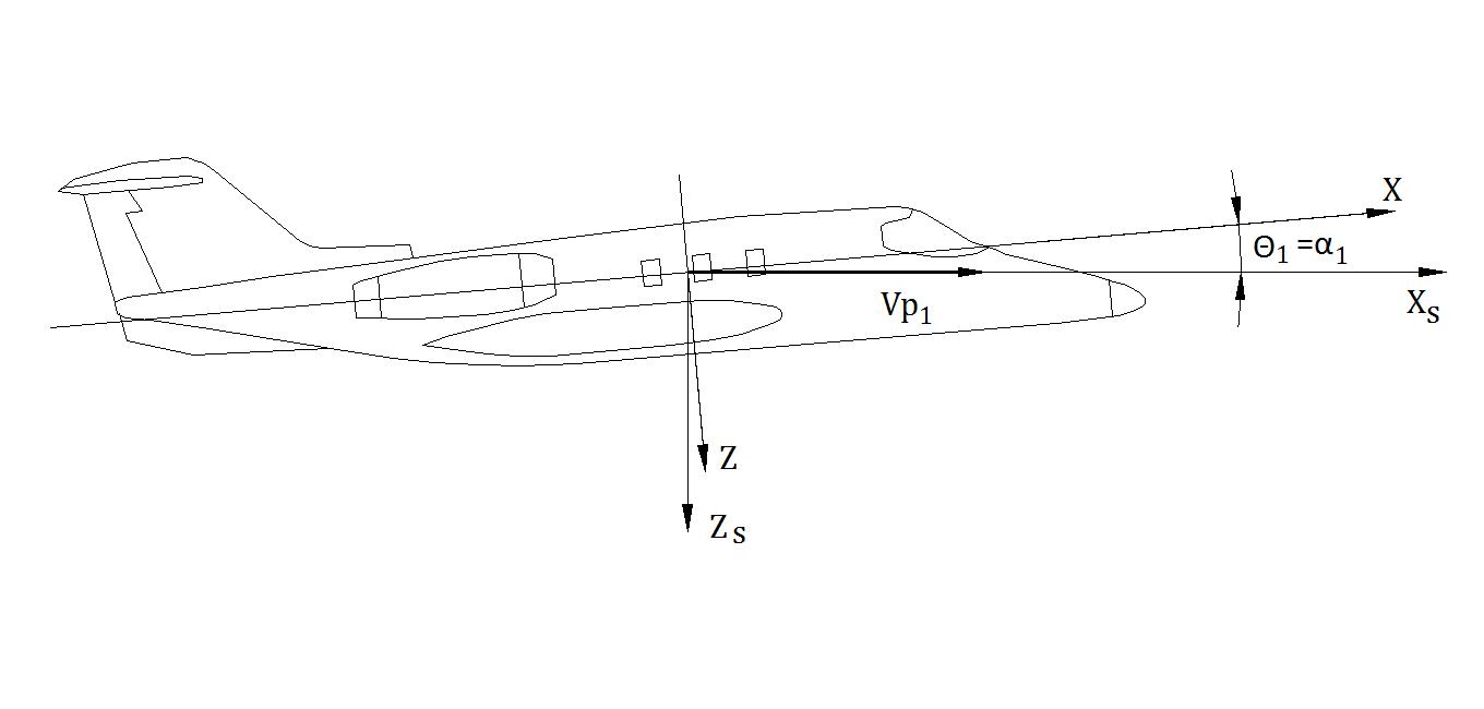
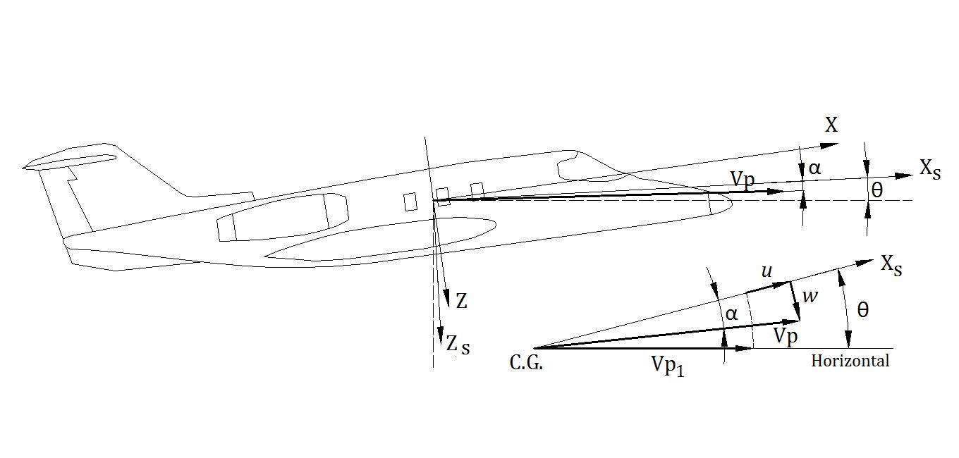
Then,

Figure 8.14.4 - Dynamic variables at an arbitrary time

Since (),(),() uttt  are known for any time t, then the required velocity can be obtained.

Figure P8.14.5 shows the associated results.

Figure P8.14.5 - Velocity components along the Earth-Fixed reference for the Learjet 24

Flight Path

The flight path can be determined by integrating numerically the aircraft velocity and using the following approximation:

Thus,

The initial conditions

'(0) Z is negative since the Z‟ axis points downwards.

Figure P8.14.6 shows the flight path; note that –Z was used in the vertical axis to relate it directly with the flight altitude. A sampling time t of 0.1 sec. was used.

FlightPath

P8.14.6 - Flight path for the Learjet 24

Flight Path Angle. -Approach 1. From Figure P8.14.2 it can be seen that at steady state in each time interval:

-Approach 2. From Figure P8.14.6 it can be seen that at steady state in each time interval:

Figure

Note that the results obtained with the two approaches virtually over lap each other. Finally, the required table is presented below. The altitude trend at each time interval is obtained from Figure P8.14.6. The steady state pitch angle at each time interval is obtained as 1 ssss  ; similarly, The steady state aircraft angle of attack at each time interval is obtained as 1

 . The steady state horizontal velocity is obtained from Figure P8.14.5. The sign of the steady state vertical velocity can be determined from Figure P8.14.5 or estimated from Figure P8.14.6.

Table P8.14.2 - Value of the dynamic variables at steady state in each time interval for the Learjet 24

Note that when the angle of attack decreases, the aircraft lift coefficient decreases, and the velocity increases. Also, note that during the maneuver the thrust is held constant.