Issuu

by Jordan, Miller, Dolvin

ISBN: 9781265417888

Chapter 1 A Brief History of Risk and Return

Concept Questions

1. For both risk and return, increasing order is b, c, a, d. On average, the higher the risk of an investment, the higher is its expected return.

2. Since the price didn’t change, the capital gains yield was zero. If the total return was four percent, then the dividend yield must be four percent.

3. It is impossible to lose more than 100 percent of your investment. Therefore, return distributions are cut off on the lower tail at 100 percent; if returns were truly normally distributed, you could lose much more.

4. To calculate an arithmetic return, you sum the returns and divide by the number of returns. As such, arithmetic returns do not account for the effects of compounding (and, in particular, the effect of volatility). Geometric returns do account for the effects of compounding and for changes in the base used for each year’s calculation of returns. As an investor, the more important return of an asset is the geometric return.

5. Blume’s formula uses the arithmetic and geometric returns along with the number of observations to approximate a holding period return. When predicting a holding period return, the arithmetic return will tend to be too high andthe geometric return will tend to be toolow. Blume’s formula adjuststhese returns for different holding period expected returns.

6. T-bill rates were highest in the early eighties since inflation at the time was relatively high. As we discuss in our chapter on interest rates, rates on T-bills will almost always be slightly higher than the expected rate of inflation.

7. Risk premiums are about the same regardless of whether we account for inflation. The reason is that risk premiums are the difference between two returns, so inflation essentially nets out.

8. Returns, risk premiums, and volatility would all be lower than we estimated because aftertax returns are smaller than pretax returns.

9. We have seen that T-bills barely kept up with inflation before taxes. After taxes, investors in T-bills actually lost ground (assuming anything other than a very low tax rate). Thus, an all T-bill strategy will probably lose money in real dollars for a taxable investor.

10. It is important not to lose sight of the fact that the results we have discussed cover over 80 years, well beyond the investing lifetime for most of us. There have been extended periods during which small stocks have done terribly. Thus, one reason most investors will choose not to pursue a 100 percent stock (particularly small-cap stocks) strategy is that many investors have relativelyshort horizons, and high volatility investments may be very inappropriate in such cases. There are other reasons, but we will defer discussion of these to later chapters.

McGrawHillLLC.Allrightsreserved.NoreproductionordistributionwithoutthepriorwrittenconsentofMcGraw Hill LLC.

Solutions to Questions and Problems

NOTE: All end of chapter problems were solved using a spreadsheet. Many problems require multiple steps. Due to space and readability constraints, when these intermediate steps are included in this solutions manual, rounding may appear to have occurred. However, the final answer for each problem is found without rounding during any step in the problem.

Core Questions

1. Total dollar return = 100($41 $37 + $.28) = $428.00 Whether you choose to sell the stock does not affect the gain or loss for the year; your stock is worth what it would bring if you sold it. Whether you choose to do so or not is irrelevant (ignoring commissions and taxes).

2. ( ) Capitalgainsyield $41 – $37/$37 .1081, or10.81% == Dividendyield $.28/$37 .0076, or.76% ==

3. Dollar return = 500($34 $37 + $.28) = $1,360 ( ) Capitalgainsyield $34 – $37/$37 –.0811,or –8.11% ==

.0076, or.76%

a. average return = 6.0%, average risk premium = 2.7%

b. average return = 3.3%, average risk premium = 0%

c. average return =

McGrawHillLLC.Allrightsreserved.NoreproductionordistributionwithoutthepriorwrittenconsentofMcGraw Hill LLC.

Intermediate Questions

10. That’s plus or minus one standard deviation, so about two-thirds of the time, or two years out of three. In one year out of three, you will be outside this range, implying that you will be below it one year out of six and above it one year out of six.

11. You lose money if you have a negative return. With a 12 percent expected return and a 6 percent standard deviation, a zero return is two standard deviations below the average. The odds of being outside (above or below) two standard deviations are 5 percent; the odds of being below are half that, or 2.5 percent. (It’s actually 2.28 percent.) You should expect to lose money only 2.5 years out of every 100. It’s a pretty safe investment.

12. The average return is 6.0 percent, with a standard deviation of 9.8 percent, so Prob(Return < 3.8 or Return 15.8 1/3 )  , but we are only interested in one tail; ( ) ProbReturn –3.9 1/6,  which is half of 1/3 (or about 16%)

95%: 6.0 ± 2σ = 6.0 ± 2(9.8) = 13.6% to 25.6%

99%: 6.0 ± 3σ = 6.0 ± 3(9.8) = 23.4% to 35.4%

13. Expected return = 16.4%; σ = 31.2%. Doubling your money is a 100% return, so if the return distribution is normal, ( ) 100 – 16.4/31.2 2.68 Z == standard deviations; this is in-between two and three standard deviations, so the probability is small, somewhere between .5% and 2.5% (why?). Referring to the nearest Z table, the actual probability is = 0.369%, or less than every 100 years. Tripling your money would be ( ) 200 – 16.4/31.2 5.88 Z == standard deviations; this corresponds to a probability of (much) less than 0.01%. (The actual answer is less than once every 1 million years, so don’t hold your breath.)

14.

a. Annual risk premium = Common stock return T-bill return (see table above).

b. Averagereturns:Commonstocks 12.84/5 .0257, or 2.57%; T-bills 31.67/5 .0633, or 6.33%

–18.83/5 –.0377, or –3.77%

) ( ) 22 .2393 – .0257 –.0717 ] 6 –

( )1/2

0.072337 .2690,or26.90%

–

– .0257

c. ( ) ( ) ( ) 222 Commonstocks:Var 1/4 –.1469 – .02 [

T-bills: Var = 1/4[( 0729 0633)2 + ( 0799 0633)2 + ( 0587 0633)2 + (.0507 .0633)2 + (.0545 .0633)2] = .000156 ( )1/2

Standarddeviation .000156 .0125,or1.25% ==

Standarddeviation .077446 .2783,or27.83% ==

Riskpremium:Var = 1/4[( 2198 ( 0377))2 + ( 3446 ( 0377))2 + ( 3136 ( 0377))2 +( 1886 ( 0377))2 + ( .1261 ( .0377))2] = .077446 ( )1/2

d. Before the fact, for most assets the risk premium will be positive; investors demand compensation over and above the risk-free return to invest their money in the risky asset. After the fact, the observed risk premium can be negative if the asset’s nominal return is unexpectedly low, the riskfree return is unexpectedly high, or any combination of these two events.

15. ( )1/50 $324,000/$1,000– 1 .1226, or12.26% =

17. Small-companystocks =($61,81603/$1)1/99 1 = 1179,or1179% Large-companystocks = ($17,894.03/$1)1/99 1

5 ©McGrawHillLLC.Allrightsreserved.NoreproductionordistributionwithoutthepriorwrittenconsentofMcGraw Hill LLC.

The larger the standard deviation, the greater will be the difference between the arithmetic return and geometric return. In fact, for lognormally distributed returns, another formula to find the geometric returnis: arithmeticreturn –½ variance.Therefore,forStockC,weget ( ) .0800–½.047950.0560. =

The difference in this case is because the return sample is not a true lognormal distribution.

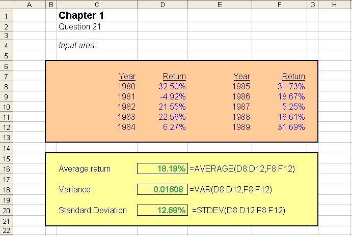
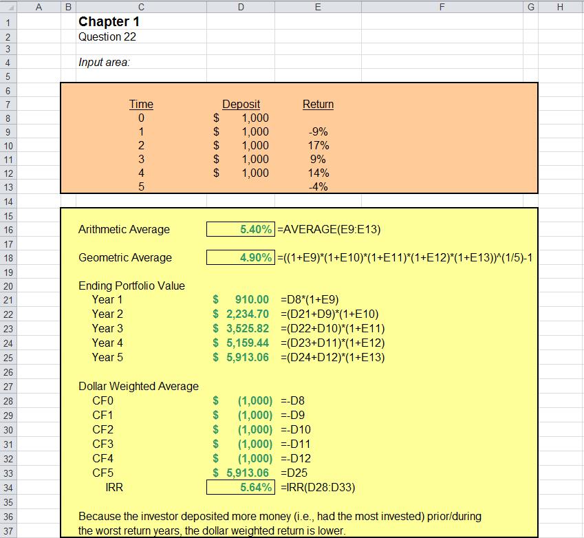
Spreadsheet Problems 21.

McGrawHillLLC.Allrightsreserved.NoreproductionordistributionwithoutthepriorwrittenconsentofMcGraw Hill LLC.

CFA Exam Review by Schweser 1. a

Scenario 2 Ending MV

of Year 2 = 100(.9)(1.25) + 20 = 132.5

Scenario 3 Ending MV

of Year 2 = 100(.9)(1.25) 10 = 102.5

3. c ( )12

4. b

Geometric returns provide the best estimate of a portfolio manager’s return because it neutralizes theimpact oftheclient’s cash flow decisions. Fortheclients themselves, the dollar-weighted return would be appropriate.

Chapter 1 A Brief History of Risk and Return

Chapter Organization

1.1 Returns

A. Dollar Returns

B. Percentage Returns

C. A Note on Annualizing Returns

1.2 The Historical Record

A. A First Look

B. A Longer Range Look

C. A Closer Look

D. 2008: The Bear Growled and Investors Howled

1.3 Average Returns: The First Lesson

A. Calculating Average Returns

B. Average Returns: The Historical Record

C. Risk Premiums

D. The First Lesson

1.4 Return Variability: The Second Lesson

A. Frequency Distributions and Variability

B. The Historical Variance and Standard Deviation

C. The Historical Record

D. Normal Distribution

E. The Second Lesson

1.5 More on Average Returns

A. Arithmetic versus Geometric Averages

B. Calculating Geometric Average Returns

C. Arithmetic Average Return or Geometric Average Return?

D. Dollar-Weighted Average Returns

1.6 Risk and Return

A. The Risk-Return Trade-off

B. A Look Ahead

1.7 Summary and Conclusions

Selected Web Sites

• finance.yahoo.com (basic financial information all free)

• www.globalfinancialdata.com (reference for historical financial market data not free)

• robertniles.com/stats (review of basic statistics)

Annotated Chapter Outline

1.1

Returns

This chapter uses financial market history to provide information about risk and return. In general, two key observations emerge:

• There is a reward for bearing risk and, on average, the reward has been considerable.

• Greater rewards are accompanied by greater risks.

The important point is that risk and return are always linked together.

A. Dollar Returns

Total dollar return: the return on an investment measured in dollars that accounts for all cash flows and capital gains or losses.

When you buy an asset, your gain or loss is called the return on your investment. This return is made up of two components:

• The cash you receive while you own the asset (interest or dividends), and

• The change in value of the asset, the capital gain or loss.

The total dollar return is the sum of the cash received and the capital gain or loss on the investment. Whether you sell the stock or not, this is a real gain because you had the opportunity to sell the stock at any time.

B. Percentage Returns

Total percent returns: the return on an investment measured as a percentage of the original investment that accounts for all cash flows and capital gains or losses

When you calculate percent returns, your return doesn't depend on how much you invested. Percent returns tell you how much you receive for every dollar invested. There are two components of the return:

• Dividend yield, the current dividend divided by the beginning price

• Capital gains yield, the change in price divided by the beginning price

C. A Note on Annualizing Returns

To compare investments, we need to “annualize” the returns, which we refer to as the Effective Annual Return (or EAR).

1 + EAR = (1 + holding period return)m

Where m is the number of holding periods in a year.

1.2 The Historical Record

The year-to-year historical rates of return on five important categories of investments are analyzed in this section. These categories are:

• Large-company stocks, which is based on the Standard & Poor’s 500 index (S&P 500).

• Small-company stocks, where "small" corresponds to the smallest 20% of the companies listed on the major U.S. exchanges, as measured by the market value of outstanding stock.

• Long-term corporate bonds, which is a portfolio of high-quality bonds with 20 years to maturity.

• Long-term U.S. government bonds, which is a portfolio of U.S. government bonds with 20 years to maturity.

• U.S. Treasury bills (T-bills) with a three-month life.

The annual percentage changes in the Consumer Price Index (CPI) are also calculated as a comparison to consumer goods price inflation.

A. A First Look

When we examine the returns on these categories of investments from 1926 through 2024, we see that the small-company investment grew from $1 to $61,816.03, the large-company stock portfolio to $17,894.03. At the other extreme, the T-bills only grew to $24.46. Inflation caused the price of an average consumer good to grow from $1 to $17.65. An obvious question resulting from examining this graph would be, “Why would anyone invest in anything other than

small-company stocks?” The answer lies in the higher volatility of the smallcompany stocks. This topic will be discussed later in the chapter.

B. A Longer Range Look

When we look at a longer term, back to 1801, we see that the return from investing in stocks is much higher than investing in bonds or gold. Over this 224year period, one dollar invested in stocks grew to an astounding $72.68 million, whereas gold has slightly outperformed inflation. The moral is, “Start investing early.”

C. A Closer Look

As you examine the bar graphs, you can observe that the return on stocks, especially small-company stocks, was much more variable than bonds or T-bills.

The returns on T-bills were much more predictable than stocks. Although the largest one-year return was 153% for small-company stocks and 53% for largecompany stocks, the largest T-bill return was only 14.6%. The largest historical return for long-term government bonds was 47.14%, which occurred in 1982

D. 2008: The Bear Growled and Investors Howled

The S&P 500 index plunged 37 percent in 2008, which is behind only 1931, which was at 44 percent. Moreover, there were 18 days during 2008 on which the value of the S&P changed by more than 5 percent. From 1956 to 2007, there were only 17 such days.

1.3 Average Returns: The First Lesson

This section provides simple measures to accurately summarize and describe all these numbers, starting with calculating average returns.

A. Calculating Average Returns

The simplest way to calculate average returns is to add the annual returns and divide by the number of years. This will provide the historical average. So, the average return for the large-company stocks over the 99 years is 12.3%.

B. Average Returns: The Historical Record

Table 1.2 also shows that small-company stocks had an average return of 16.0%, government bonds returned 5.5%, and T-bills only returned 3.3%. Note that the return on T-bills is slightly more than the inflation rate of 3.0%.

C. Risk Premiums

Risk-free rate: the rate of return on a riskless investment.

Risk premium: the extra return on a risky asset over the risk-free rate.

The rate of return on T-bills is essentially risk free because there is no risk of default. So, we will use T-bills as a proxy for the risk-free rate, our investing benchmark. If we consider T-bills as risk-free investing and investing in stocks as risky investing, the difference between these two returns would be the risk premium for investing in stocks. This is the additional return we receive for investing in the risky asset, or the reward for bearing risk.

The U.S. Equity Risk Premium: Historical and International Perspectives: Earlier periods suggest a lower risk premium than in recent periods, while international risk premiums also tend to be slightly lower. Based on evidence and expectations, 7 percent seems to be a reasonable estimate for the risk premium.

D. The First Lesson

When we calculate the risk premium for large-company stocks (stock return minus the T-bill return) we get 9.0% and for government bonds 2.2%. Of course, the risk premium for T-bills is zero. So, we see that risky assets, on average, earn a risk premium, or “there is a reward for bearing risk.” The next question is, “Why is there a difference in the risk premiums?” This is addressed in the next section and relates to the variability in returns.

1.4 Return Variability: The Second Lesson

A. Frequency Distributions and Variability

Variance: a common measure of volatility.

Standard deviation: the square root of the variance.

Variance and standard deviation provide a measure of return volatility or how much the actual return differs from this average in a typical year. This is the same variance and standard deviation discussed in statistics courses.

B. The Historical Variance and Standard Deviation

The variance measures the average squared difference between the actual returns and the average return. The larger this number, the more the actual returns differ from the average return. Note how the stocks have a much larger standard deviation than the bonds and were therefore more volatile.

Lecture Tip: Although all students should have been exposed to calculating variance and standard deviation, many still have difficulty with it. Another method to illustrate how to calculate the variance is to structure it in the form of a table

where each step is a separate column. This is illustrated below using the data in the text.

For 1926-1930, the average return for large-company stocks (as represented by the S&P 500) = (11.14% + 37.13% + 43.31% 8.91% 25.26%)/5 = 57.41%/5 = 11.48%

of squares = 3,436.77 (RN - RA)2/(N-1) = 3,436.77/(5-1) = 859.19 Variance

Square root = 29.31% Standard deviation

Lecture Tip: Note the difference between using N-1 and N as the divisor when calculating variance and standard deviation. You use N when you have the entire population, as opposed to N-1 when you have a sample of the population.

Lecture Tip: After calculating variance and standard deviation, ask what units are attached to each. The students will most likely have to puzzle on this. Of course, variance is percent squared, whereas standard deviation is percent. This provides a starting point for the discussion on how to interpret the resulting value for standard deviation.

Lecture Tip: You may want to point out that this example calculates variance and standard deviation using historical data. When expected futures values are used, there is another method that must employ probabilities. This method will be discussed in a later chapter.

C. The Historical Record

The standard deviation for the large-company stock portfolio is more than six times the standard deviation for the T-bill portfolio. Also notice that the distribution is approximately normal. This allows us to use the fact that plus or minus one standard deviation from the mean return gives us the range of returns that would result 2/3 of the time. If we take plus or minus two standard deviations from the mean, there is a 95% probability that our investment will be within this range of returns.

D. Normal Distribution

Like most statistical concepts, students will struggle remembering the concept of a normal distribution. In our experience, this is mostly because they are unsure of their understanding not that they have not “seen” the material before.

For many different random events in nature, a particular frequency distribution, the normal distribution (or bell curve) is useful for describing the probability of ending up in a given range. For example, the idea behind “grading on a curve” comes from the fact that exam scores often resemble a bell curve.

Figure 1.10 illustrates a normal distribution and its distinctive bell shape. As you can see, this distribution has a much cleaner appearance than the actual return distributions illustrated in Figure 1.8. Even so, like the normal distribution, the actual distributions do appear to be at least roughly mound shaped and symmetric. When this is true, the normal distribution is often a very good approximation.

Also, you will have to remind students that the distributions in Figure 1.8 are based on only 99 yearly observations, while Figure 1.10 is, in principle, based on an infinite number. So, if we had been able to observe returns for, say, 1,000 years, we might have filled in a lot of the irregularities and ended up with a much smoother picture. For our purposes, it is enough to observe that the returns are at least roughly normally distributed.

The usefulness of the normal distribution stems from the fact that it is completely described by the average and the standard deviation. If you have these two numbers, then there is nothing else to know. For example, with a normal distribution, the probability that we end up within one standard deviation of the average is about 2/3. The probability that we end up within two standard deviations is about 95 percent. Finally, the probability of being more than three standard deviations away from the average is less than 1 percent.

E. The Second Lesson

Observing that there is variability in returns from year-to-year, we see that there is a significant chance of a large change in value in the returns. So, the second lesson is: The greater the potential reward, the greater the risk.

1.5 More on Average Returns

A. Arithmetic versus Geometric Averages

The geometric average return answers the question: “What was your average compound return per year over a particular period?”

The arithmetic average return answers the question: “What was your return in an average year over a particular period?”

B. Calculating Geometric Average Returns

Let us use data from the example above to calculate an arithmetic average and a geometric average:

C. Arithmetic Average Return or Geometric Average Return?

Two points are worth stressing:

First, generally, when one sees a discussion of “average returns,” the return in question is an arithmetic return.

Second, there is a nettlesome problem concerning forecasting future returns using estimates of arithmetic and geometric returns. The problem is: arithmetic average returns are probably too high for longer periods, and geometric average returns are probably too low for shorter periods. Fortunately, Blume’s formula provides a way to weight arithmetic and geometric averages for a T-year average return forecast using arithmetic and geometric averages which have been calculated for an N-year period (T cannot exceed N).

As is clear from this formula, as T (the length of time of the forecast) increases, the geometric average receives a higher weight relative to the arithmetic average. That is, if N = T, the arithmetic average receives no weight, and the resulting forecast stems entirely from the geometric average. If T = 1, then the geometric average receives a zero weight. In this case, the resulting forecast comes only from the arithmetic average.

D. Dollar-Weighted Average Returns

If an investor adds money to or subtracts money from an account, his actual return will likely be different than either the arithmetic or geometric average. The dollar weighted return (or internal rate of return, IRR) captures the impact of cash flows, giving the average compound rate of return earned per year.

1.6 Risk and Return

A. The Risk-Return Trade-off

If we are unwilling to take on any risk, but we are willing to forego the use of our money for a while, then we can earn the risk-free rate. We can think of this as the time value of money. If we are willing to bear risk, then we can expect to earn a risk premium, on average. We can think of these two factors as the “wait” component and the “worry” component.

Notice that the risk premium is not guaranteed; it is “on average.” Risky investments by their very nature of being risky do not always pay more than riskfree investments. Also, only those risks that are unavoidable are compensated by the risk premium. There is no reward for bearing avoidable risk.

B. A Look Ahead

The remainder of the text focuses on financial assets only: stocks, bonds, options and futures. Remember that to understand the potential reward from an investment, you must understand the risk involved.