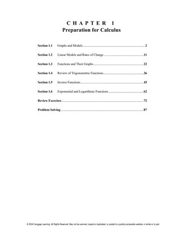
C H A P T E R 1 Preparation for Calculus Section 1.1
Graphs and Models................................................................................. 2
Section 1.2
Linear Models and Rates of Change ................................................... 11
Section 1.3
Functions and Their Graphs ................................................................. 22
Section 1.4
Review of Trigonometric Functions .................................................... 36
Section 1.5
Inverse Functions.................................................................................. 45
Section 1.6
Exponential and Logarithmic Functions ............................................. 62
Review Exercises .......................................................................................................... 72 Problem Solving ........................................................................................................... 87
© 2024 Cengage Learning. All Rights Reserved. May not be scanned, copied or duplicated, or posted to a publicly accessible website, in whole or in part.
C H A P T E R 1 Preparation for Calculus Section 1.1 Graphs and Models 1. To find the x-intercepts of the graph of an equation, let y be zero and solve the equation for x. To find the y-intercepts of the graph of an equation, let x be zero and solve the equation for y.
8. y = 5 − 2 x x
−1
0
1
2
5 2
3
4
y
7
5
3
1
0
−1
−3
2. Symmetry helps in sketching a graph because you need only half as many points to plot. Answers will vary. 3. y = − 32 x + 3 x-intercept: ( 2, 0) y-intercept: (0, 3) Matches graph (b). 9. y = 4 − x 2
9 − x2
4. y =
x-intercepts: ( −3, 0), (3, 0)
x
−3
−2
0
2
3
y-intercept: (0, 3)
y
−5
0
4
0
−5
Matches graph (d). 5. y = 3 − x 2 x-intercepts:
( 3, 0), (− 3, 0)
y-intercept: (0, 3) Matches graph (a). 6. y = x3 − x x-intercepts: (0, 0), ( −1, 0), (1, 0)
10. y = ( x − 3)
2
y-intercept: (0, 0)
x
0
1
2
3
4
5
6
Matches graph (c).
y
9
4
1
0
1
4
9
7. y = 12 x + 2
2
x
−4
−2
0
2
4
y
0
1
2
3
4
© 2024 Cengage Learning. All Rights Reserved. May not be scanned, copied or duplicated, or posted to a publicly accessible website, in whole or in part.
Section 1.1 11. y = x + 1
15. y =
x
−4
−3
−2
−1
0
1
2
y
3
2
1
0
1
2
3
Graphs and Models
3
3 x
x
−3
−2
−1
0
1
2
3
y
−1
− 32
−3
Undef.
3
3 2
1
12. y = x − 1 x
−3
−2
−1
0
1
2
3
y
2
1
0
−1
0
1
2
13. y =
16. y = x
−6
−4
−3
−2
−1
0
2
y
− 14
− 12
−1
Undef.
1
1 2
1 4
x −6
x
0
1
4
9
16
y
−6
−5
−4
−3
−2
17. y =
(a)
14. y =
1 x + 2
5− x
(2, y) = ( 2, 1.73)
(b) ( x, 3) = ( −4, 3)
x + 2
x
−2
−1
0
2
7
14
y
0
1
2
2
3
4
(y =
(3 =
5−2 = 5 − ( −4)
)
3 ≈ 1.73
)
18. y = x5 − 5 x
(a)
(−0.5, y) = (−0.5, 2.47)
(b) ( x, − 4) = ( −1.65, − 4) and ( x, − 4) = (1, − 4)
© 2024 Cengage Learning. All Rights Reserved. May not be scanned, copied or duplicated, or posted to a publicly accessible website, in whole or in part.
4
Chapter 1
Preparation for Calculus
19. y = 2 x − 5 y-intercept: y = 2(0) − 5 = −5; (0, − 5) x-intercept: 0 = 2 x − 5
5 = 2x x = 52 ;
( 52 , 0)
25. y =
2− x 5x + 1
y -intercept: y =
2− 0 = 2; 5(0) + 1
x-intercept: 0 =
2− x 5x + 1
20. y = 4 x 2 + 3
y-intercept: y = 4(0) + 3 = 3; (0, 3) 2
x-intercept: 0 = 4 x 2 + 3
26. y =
−3 = 4 x 2 None. y cannot equal 0.
0 = 2−
x
x = 4;
(4, 0)
x 2 + 3x
(3x + 1)
2
y-intercept: y =
21. y = x 2 + x − 2
0 = ( x + 2)( x − 1) x = −2, 1; ( −2, 0), (1, 0)
y = 0; (0, 0) x-intercepts: 0 = x3 − 4 x 0 = x( x − 2)( x + 2)
2
x 2 + 3x
(3x + 1) x( x + 3) 0 = 2 (3x + 1) x = 0, − 3; (0, 0), ( −3, 0)
x-intercepts: 0 = x + x − 2
y-intercept: y 2 = 03 − 4(0)
3(0) + 1
x-intercepts: 0 =
2
22. y 2 = x3 − 4 x
02 + 3(0)
y = 0; (0, 0)
y-intercept: y = 02 + 0 − 2
y = −2; (0, − 2)
2
27. x 2 y − x 2 + 4 y = 0
y-intercept: 02 ( y ) − 02 + 4 y = 0 y = 0; (0, 0) x-intercept: x 2 (0) − x 2 + 4(0) = 0 x = 0; (0, 0)
x = 0, ± 2; (0, 0), ( ± 2, 0) 28. y = 2 x −
23. y = x 16 − x 2
y-intercept: y = 0 16 − 02 = 0; (0, 0) x-intercepts: 0 = x 16 − x 2
(4 − x)(4 + x) x = 0, 4, − 4; (0, 0), ( 4, 0), ( − 4, 0)
0 = x
x2 + 1
y-intercept: y = 2(0) −
x-intercept:
0 = 2x − 4x2 = x2 + 1
y-intercept: y = (0 − 1) 02 + 1
x2 =
x-intercept: 0 = ( x − 1)
x = 1; (1, 0)
x2 + 1
x2 + 1
2x = 3x 2 = 1
y = −1; (0, −1)
02 + 1
y = −1; (0, −1)
x2 + 1
24. y = ( x − 1)
(0, 2)
1 3
x = ±
3 3
x =
3 3 ; , 0 3 3
x2 + 1
Note: x = − 3 3 is an extraneous solution.
© 2024 Cengage Learning. All Rights Reserved. May not be scanned, copied or duplicated, or posted to a publicly accessible website, in whole or in part.
Section 1.1 29. Symmetric with respect to the y-axis because y = ( − x) − 6 = x − 6. 2
2
Graphs and Models
5
41. y = 2 − 3 x y = 2 − 3(0) = 2, y -intercept 0 = 2 − 3( x) 3 x = 2 x = 23 , x-intercept
30. y = 9 x − x 2 No symmetry with respect to either axis or the origin. 31. Symmetric with respect to the x-axis because
Intercepts: (0, 2),
( 23 , 0)
Symmetry: none
(− y )2 = y 2 = x3 − 8 x. 32. Symmetric with respect to the origin because
( − y ) = ( − x )3 + ( − x ) − y = − x3 − x 42. y = 23 x + 1
y = x3 + x. 33. Symmetric with respect to the origin because ( − x)( − y ) = xy = 4. 34. Symmetric with respect to the x-axis because x( − y ) = xy = −10. 2
2
35. y = 4 −
y = 23 (0) + 1 = 1, y -intercept 0 = 23 x + 1 − 23 x = 1 x = − 32 , x-intercept
(
Intercepts: (0, 1), − 32 , 0
)
Symmetry: none
x +3
No symmetry with respect to either axis or the origin. 36. Symmetric with respect to the origin because
(− x)(− y ) −
4 − ( − x) = 0 2
xy −
4− x
2
= 0.
37. Symmetric with respect to the origin because −y =
−x
43. y = 9 − x 2 y = 9 − (0) = 9, y -intercept 2
0 = 9 − x 2 x 2 = 9 x = ± 3, x-intercepts Intercepts: (0, 9), (3, 0), ( −3, 0)
( − x) + 1 2
y = 9 − (− x) = 9 − x 2 2
x y = 2 . x +1
Symmetry: y-axis
38. Symmetric with respect to the origin because
−y =
( − x) 2 4 − ( − x)
−y =
− x5 4 − x2
5
44. y = 2 x 2 + x = x( 2 x + 1)
y = 0( 2(0) + 1) = 0, y -intercept
x5 . y = 4 − x2
0 = x( 2 x + 1) x = 0, − 12 , x-intercepts
39. y = x 3 + x is symmetric with respect to the y-axis because y = ( − x) + ( − x) = −( x3 + x) = x3 + x . 3
40.
(
Intercepts: (0, 0), − 12 , 0
)
Symmetry: none
y − x = 3 is symmetric with respect to the x-axis
because
−y − x = 3 y − x = 3.
© 2024 Cengage Learning. All Rights Reserved. May not be scanned, copied or duplicated, or posted to a publicly accessible website, in whole or in part.
6
Chapter 1
Preparation for Calculus
45. y = x3 + 2 y = 03 + 2 = 2, y -intercept 0 = x + 2 x = −2 x = − 3
3
(
Intercepts: −
25 − x 2
48. y =
3
25 − 02 =
y = 3
2, x-intercept
25 − x 2 = 0
)
2, 0 , (0, 2)
Symmetry: none
25 = 5, y -intercept
25 − x 2 = 0
(5 + x)(5 − x) = 0 x = ± 5, x -intercept Intercepts: (0, 5), (5, 0), ( −5, 0)
y =
25 − ( − x) = 2
25 − x 2
Symmetry: y-axis
46. y = x 3 − 4 x
y = 03 − 4(0) = 0, y -intercept x3 − 4 x = 0 x ( x 2 − 4) = 0 x( x + 2)( x − 2) = 0 x = 0, ± 2, x -intercepts Intercepts: (0, 0), ( 2, 0), ( −2, 0) y = ( − x ) − 4( − x ) = − x 3 + 4 x = −( x 3 − 4 x) 3
Symmetry: origin
49. x = y 3
y 3 = 0 y = 0, y -intercept x = 0, x-intercept Intercept: (0, 0) − x = (− y ) − x = − y 3 3
Symmetry: origin
50. x = y 4 − 16 y 4 − 16 = 0
( y 2 − 4)( y 2 + 4) = 0 ( y − 2)( y + 2)( y 2 + 4) = 0 y = ± 2, y -intercepts
47. y = x
x +5
y = 0 0 + 5 = 0, y -intercept x
x + 5 = 0 x = 0, − 5, x-intercepts
Intercepts: (0, 0), ( −5, 0)
x = 0 4 − 16 = −16, x -intercept
Intercepts: (0, 2), (0, − 2), ( −16, 0) Symmetry: x-axis because x = ( − y ) − 16 = y 4 − 16 4
Symmetry: none
© 2024 Cengage Learning. All Rights Reserved. May not be scanned, copied or duplicated, or posted to a publicly accessible website, in whole or in part.
Section 1.1
51. y =
8 x
7
54. y = 6 − x
8 y = Undefined no y -intercept 0 8 = 0 No solution no x-intercept x
Intercepts: none −y =
Graphs and Models
8 8 y = −x x
y = 6 − 0 = 6 = 6, y -intercept
6− x = 0 6− x = 0 6 = x, x-intercept Intercepts: (0, 6), (6, 0) Symmetry: none
Symmetry: origin
55. x 2 + y 2 = 9 y2 = 9 − x2
52. y = y =
10 x2 + 1 10 = 10, y -intercept 0 +1 2
10 = 0 No solution no x-intercepts 2 x +1
Intercept: (0, 10)
10
10 y = = 2 2 x +1 ( − x) + 1 Symmetry: y-axis
y = ± 9 − x2 y = ± 9 − 0 = ±3, y -intercepts ± 9− x
2
= 0
2
9− x = 0 9 = x2 ±3 = x, x-intercepts Intercepts: ( ±3, 0), (0, ± 3)
( − x)2 + y 2 = 9 x 2 + y 2 = 9 x2 + (− y) = 9 x 2 + y 2 = 9 2
(− x)2 + ( − y )2 = 9 x 2 + y 2 = 9 53. y = 6 − x
Symmetry: x-axis, y-axis, origin
y = 6 − 0 = 6, y -intercept
6− x = 0 6 = x x = ± 6, x-intercepts Intercepts: (0, 6), ( −6, 0), (6, 0)
y = 6 − −x = 6 − x Symmetry: y-axis
© 2024 Cengage Learning. All Rights Reserved. May not be scanned, copied or duplicated, or posted to a publicly accessible website, in whole or in part.
10
Chapter 1
Preparation for Calculus
69. (a) Using a graphing utility, you obtain
y = 0.74t + 7.2. (b)
72. y 2 = 4kx (a) (1, 1):
12 = 4k (1) 1 = 4k k = 14
(b) ( 2, 4) :
( 4)
The model is a good fit for the data. (c) For 2029, t = 29: y = 0.74( 29) + 7.2 ≈ 28.7
The GDP in 2029 will be about $28.7 trillion.
70. (a) Using a graphing utility, you obtain
(c)
(0, 0):
2
= 4k ( 2)
16
= 8k
k
= 2
0 2 = 4 k ( 0) k can be any real number.
(d) (3, 3):
(3)
y = − 0.007t 2 + 0.47t + 1.6.
2
= 4k (3)
9
= 12k
k
9 = 12 = 34
(b)
73. Answers may vary. Sample answer:
(
)
(
)
y = x + 32 ( x − 4) x − 52 has intercepts at
x = − 32 , x = 4, and x = 52 . The model is a good fit for the data. (c) For 2029, t = 29: y = − 0.007( 29) + 0.47( 29) + 1.6 ≈ 9.3 2
The number of cellphone subscriptions worldwide in 2029 will be about 9.3 billion.
71.
C = R 2.04 x + 5600 = 3.29 x 5600 = 3.29 x − 2.04 x 5600 = 1.25 x x =
5600 = 4480 1.25
To break even, 4480 units must be sold.
74. Yes. If (x, y) is on the graph, then so is ( − x, y ) by y-axis symmetry. Because ( − x, y ) is on the graph, then so is ( − x, − y ) by x-axis symmetry. So, the graph is symmetric with respect to the origin. The converse is not true. For example, y = x3 has origin symmetry but is not symmetric with respect to either the x-axis or the y-axis.
75. Yes. Assume that the graph has x-axis and origin symmetry. If (x, y) is on the graph, so is ( x, − y ) by x-axis symmetry. Because ( x, − y ) is on the graph, then so is ( − x, − ( − y )) = ( − x, y ) by origin symmetry. Therefore, the graph is symmetric with respect to the y-axis. The argument is similar for y-axis and origin symmetry.
© 2024 Cengage Learning. All Rights Reserved. May not be scanned, copied or duplicated, or posted to a publicly accessible website, in whole or in part.
Section 1.2
Linear Models and Rates of Change
11
76. (a) Intercepts for y = x 3 − x : y = 03 − 0 = 0 ; (0, 0)
y -intercept:
x -intercepts: 0 = x 3 − x = x ( x 2 − 1) = x( x − 1)( x + 1) ;
(0, 0), (1, 0) (−1, 0) Intercepts for y = x 2 + 2: y = 0 + 2 = 2 ; (0, 2)
y -intercept:
x-intercepts: 0 = x 2 + 2 None. y cannot equal 0. (b) Symmetry with respect to the origin for y = x3 − x because − y = ( − x) − ( − x) = − x 3 + x. 3
Symmetry with respect to the y-axis for y = x 2 + 2 because y = ( − x) + 2 = x 2 + 2. 2
x3 − x = x 2 + 2
(c) 3
2
x − x − x − 2 = 0
( x − 2)( x 2 + x + 1) = 0 x = 2 y = 6 Point of intersection : (2, 6)
Note: The polynomial x 2 + x + 1 has no real roots. 77 False. x-axis symmetry means that if ( − 4, − 5) is on the graph, then ( − 4, 5) is also on the graph. For example,
−b ± 79. True. The x-intercepts are
( 4, − 5) is not on the graph of x = y 2 − 29, whereas ( − 4, − 5) is on the graph.
80. True. The x-intercept is −
b 2 − 4ac , 0 . 2a
b , 0 . 2a
78. True. f ( 4) = f ( −4).
Section 1.2 Linear Models and Rates of Change 1. In the form y = mx + b, m is the slope and b is the y-intercept.
7. m =
2 − ( −4) 5−3
=
6 = 3 2
2. No. Perpendicular lines have slopes that are negative reciprocals of each other. So, one line has a positive slope and the other line has a negative slope. 3. m = 2 4. m = 0 5. m = −1 6. m = −12
© 2024 Cengage Learning. All Rights Reserved. May not be scanned, copied or duplicated, or posted to a publicly accessible website, in whole or in part.
16
Chapter 1
50. m =
Preparation for Calculus
7 −5 2 = , undefined 2 − 2 0
The line is vertical. x = 2 or x − 2 = 0
x y + =1 a −a
56.
(− 23 ) + (− 2) = 1 −a
a
−
51. The slope is
1−b 1−b = . 3− 0 3
y
=1
( ) (− 43 )
1 − b y = mx + b = x + b. 3
4 3 3x − 3 y − 4 = 0
b a
4 3
x − y =
57. The given line is vertical.
y =
−b x +b a
b x + y = b a x y + =1 a b
54.
+
The y-intercept is (0, b). Hence,
52. m = −
53.
x
2 + 2 = a 3 4 a = 3
(a) x = −7, or x + 7 = 0 (b) y = −2, or y + 2 = 0
58. The given line is horizontal. (a) y = 0 (b) x = −1, or x + 1 = 0
x y + =1 2 3 3x + 2 y − 6 = 0 x y + =1 2 − 2 − 3 − 3x y − =1 2 2 3x + y = −2
59. x + y = 7 y = −x + 7
(a)
y − 2 = −x − 3 x + y +1= 0 (b) y − 2 = 1( x + 3)
y − 2 = x +3 0 = x − y +5
3x + y + 2 = 0 x y + =1 55. 2a a 9 −2 + =1 2a a 9 − 4 =1 2a 5 = 2a 5 a = 2
x
+
y
() ()
2 52
5 2
m = −1 y − 2 = −1( x + 3)
60. x − y = − 2 y = x + 2 m =1
(a)
y − 5 = 1( x − 2) y −5 = x − 2 x − y + 3 = 0
(b)
y − 5 = −1( x − 2) y − 5 = −x + 2 x + y −7 = 0
=1
x 2y + =1 5 5 x + 2y = 5 x + 2y − 5 = 0
© 2024 Cengage Learning. All Rights Reserved. May not be scanned, copied or duplicated, or posted to a publicly accessible website, in whole or in part.
Section 1.2
61. 5 x − 3 y = 0
−6 − 4 10 = − 7 −0 7 11 − 4 7 m2 = = − −5 − 0 5 m1 ≠ m2
m = 53
(
y − 78 = 53 x − 43
(a)
)
The points are not collinear.
24 y − 21 = 40 x − 30 0 = 40 x − 24 y − 9 y − 78
(b)
17
66. m1 =
5 x 3
y =
Linear Models and Rates of Change
(
= − 53 x − 34
67.
)
40 y − 35 = −24 x + 18 24 x + 40 y − 53 = 0
62. 7 x + 4 y = 8 4 y = −7x + 8 −7 x + 2 4 7 m = − 4 y =
y +
(a)
−7 1 35 x + = 2 4 24 24 y + 12 = − 42 x + 35 42 x + 24 y − 23 = 0
y +
1 4 5 = x − 2 7 6
42 y + 21 = 24 x − 20 24 x − 42 y − 41 = 0 63. The slope is 250. V = 1850 when t = 1. V = 250(t − 1) + 1850 = 250t + 1600
64. The slope is −1600.
V = 17,200 when t = 1. V = −1600(t − 1) + 17,200 = −1600t + 18,800 65. m1 =
1−0 = −1 −2 − ( −1)
m2 =
2 −2 − 0 = − 2 − ( −1) 3
8 = 2
2.
For example, the length of segment AB is
(1 − (−1)) + (2 − 0)2 = 2
=
−7 1 5 = x − 2 4 6
y +
(b)
The four sides are of equal length:
4 + 4 8
= 2
2 units.
Furthermore, the adjacent sides are perpendicular 2 − 0 2 because the slope of AB is = = 1, whereas 1 − ( −1) 2 the slope of BC is
2 −0 = −1. 1−3
68. ax + by = 4 (a) The line is parallel to the x-axis if a = 0 and b ≠ 0. (b) The line is parallel to the y-axis if b = 0 and a ≠ 0. (c) Answers will vary. Sample answer: a = −5 and b = 8.
−5 x + 8 y = 4 y = 18 (5 x + 4) = 58 x + 12 (d) The slope must be − 52 . Answers will vary. Sample answer: a = 5 and b = 2.
5x + 2 y = 4 y = 12 ( −5 x + 4) = − 52 x + 2 (e) a = 52 and b = 3.
m1 ≠ m2
5 x + 3y = 4 2
The points are not collinear.
5x + 6 y = 8
© 2024 Cengage Learning. All Rights Reserved. May not be scanned, copied or duplicated, or posted to a publicly accessible website, in whole or in part.