JasonInvesting WeeklyInvestment Overview_2024-03_ISSUE 3

This issue, we ' re covering:

Weekly Investment Overview

Dear Subscribers,

Welcome to the JasonInvesting com Weekly Investment Overview! This week has certainly been a roller-coaster ride for investors, with unexpected twists and turns driven largely by the latest economic data The hotter-thanexpected Consumer Price Index (CPI) and Producer Price Index (PPI) reports have injected volatility into the markets, stirring up a mix of reactions across different sectors. Amidst this backdrop of fluctuating market sentiments, many of our subscribers have expressed confusion regarding our initial set of trades.

To clarify and provide insight, this week's overview will delve into one of the key strategies we employed at the initiation of our trading activities - the Bull Call Spread

Bull Call Spread Option

When we anticipate an upward movement in the market, we utilize a bull call spread strategy. This involves taking a long position on a call option with a lower strike price while simultaneously taking a short position on a call option with a higher strike price This dual approach is what defines a spread

To illustrate using an example from one of our trade recommendations:

- We go long on a 19APR24 505C

- And go short on a 19APR24 540C

One might wonder why not simply opt for a long call option if we ' re bullish on the market The rationale lies in the high premium associated with call options Incorporating a short call option helps in lowering the initial premium outlay, or net cost The extent of this reduction is influenced by the selected strike prices, a decision that involves a degree of subjectivity.

Our choice of strike prices is guided by our own proprietary time series model, which accounts for market trends and volatility

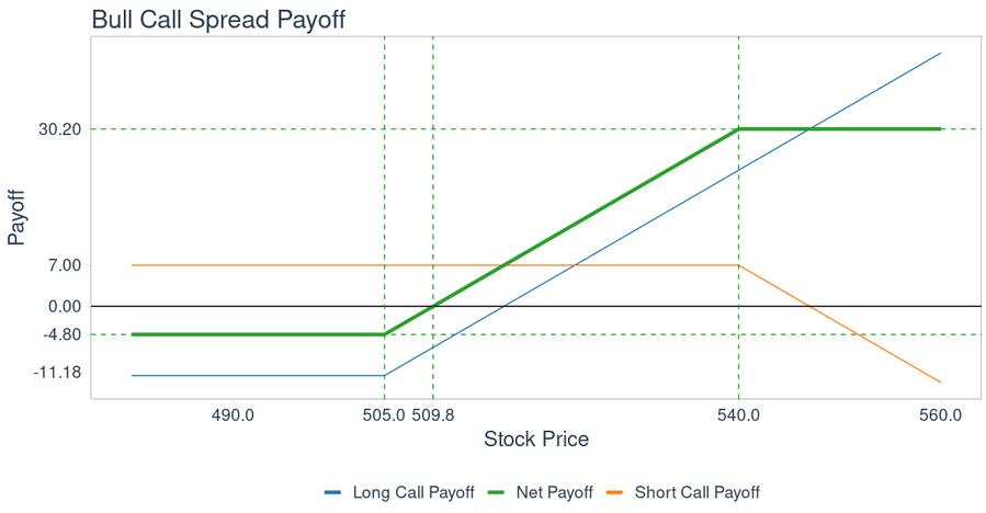
The payoff diagram for a bull call spread is usually shown as:

The payoff diagram is created by combining the outcomes from the payoff of a long call option and a short call option:

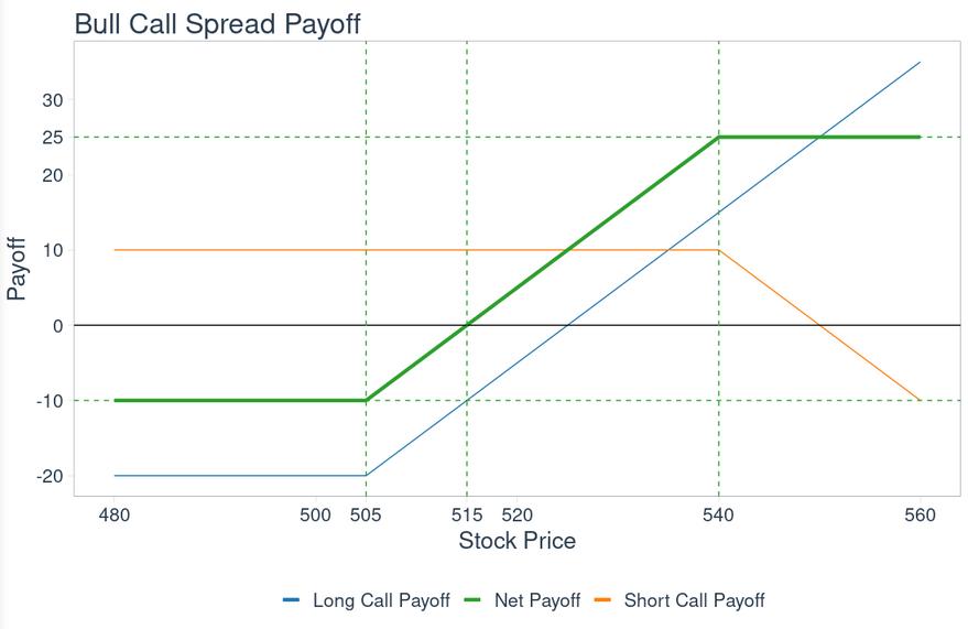
In this visualization, the payoff for the long call is depicted by the blue line, while the orange line represents the payoff for the short call.

For this example, we ' ve set the premium of the long call at a strike price of 505 to $20, and the premium of the short call at a strike price of 540 to $10 This results in a net premium outlay of $10 ($20 - $10)

The graph illustrates that the potential for profit is limited once the stock price exceeds 540; beyond this point, additional gains are not realized. To calculate the maximum profit, we subtract the strike price of the long call from that of the short call (540 - 505 = $35), and then deduct the net premium cost of $10, yielding a maximum profit of $25 The greatest possible loss is limited to the net

premium paid, which is $10. Furthermore, for the position to break even, the stock price needs to increase from 505 to at least 515, offsetting the $10 net premium cost

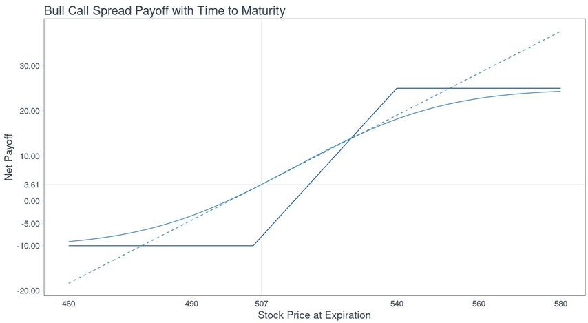
The payoff diagram as presented only accurately represents the situation at the options' expiration The actual value of the options does not follow this diagram's trajectory until they are nearing their expiry date By employing the Black-Scholes formula, we are able to illustrate how the option's payoff would appear with respect to its time-to-maturity. In this context, a time-to-maturity value of 1 corresponds to one year until maturity, whereas a value of 0 signifies the options' maturity date.

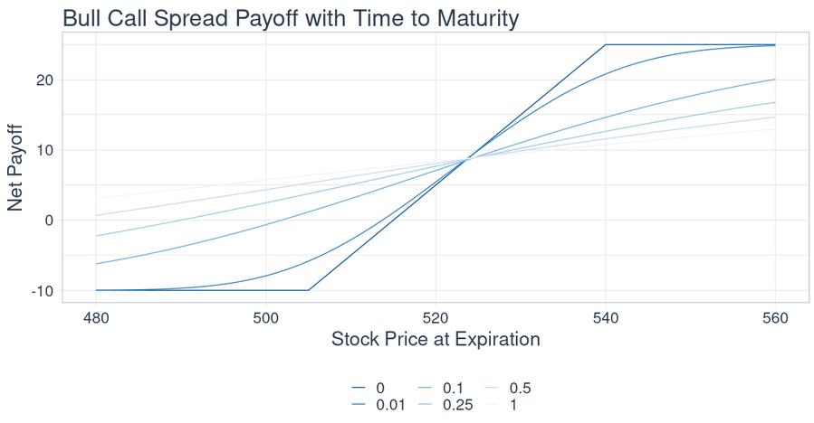
The payoff line depicted in lighter blue will ultimately merge with the darker payoff line as we approach expiration It's noticeable that the line becomes more pronounced or steeper as the time-to-maturity approaches zero. This phenomenon is related to the concept of delta, which tends to converge towards 1 between the two strike prices and drops to zero outside of this range.

Essentially, this means that as the spread nears its maturity particularly within the bounds of the two strike prices it starts to move closer to the underlying stock

Prior to this convergence, the movement of the spread will be only a portion of the underlying stock's movement. We plan to delve deeper into the intricacies of option Greeks in future issues

Let's go back and review the example with the actual premiums for the options we traded, as executed in our portfolio at the beginning

Referencing the trade details:

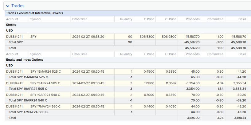
Examining the premiums for the "SPY 19APR24 505 C" at $11.18 and the "SPY 19APR24 540 C" at -$0 70, with each having a 100 multiplier for SPY options, results in a net premium expense of $1,180 ($11 18 x 100) minus $700 (-$0 70 x 100), equaling $480

This means to establish this spread, an upfront payment of $480 is required.

For breakeven, the SPY's price must reach 505 plus the premium of 4.8, totaling 509.8.

The spread's maximum loss is set at -$480, and the maximum profit potential is calculated as (540 - 505 - 4 8) x 100, which equals $3,020

Put simply, should the SPY close above 540 by expiration, our initial expenditure of $480 would yield a profit of $3,020, equating to a return of $3,020 / $480 – 1 = 5 30, or 530% return!

Yet, it's important to note that this high potential return is misleading The maximum loss is -$480, or 100%, if the SPY closes below 505, a scenario that could very well occur Consequently, investors typically risk only a small fraction of their capital to any given spread, acknowledging the possibility of a complete loss against the backdrop of a relatively high return should the trade be successful

On the trade initiation day, February 27, 2024, with the spread expiring on April 19, 2024, we find ourselves 52 days out of the 365 days, translating to a time-to-maturity of about 0.14.

For the purpose of depicting the payoff diagram prior to expiration with the Black-Scholes model, it's imperative to first determine the Implied Volatility (IV) using the given option prices

Our long option was executed at $11 18, and the short option at $0 70 When these figures are inputted into the Black-Scholes equation, the resulting IVs are 16% and 12% respectively. For those interested, a deeper dive into this calculation process could be discussed in future issues

Given that SPY closed at 507 on the day we initiated the trade, it’s also possible to calculate the delta at this specific price point

Again, applying the Black-Scholes formula,

The delta at the closing price of 507 is found to be 0 47

This delta, is lower than the 1 slope (shown as darker blue line) seen in a call spread at its expiration as seen from the chart below

When plotting this delta as a slope, it offers an insightful glimpse into the option's price sensitivity ahead of expiry

Plotting the delta as a tanget slope:

Legend: T=Time-to-Maturity

Delta (Tangent Line)

Payoff at T=0 14

Payoff at T=0 (Maturity)

SPY T=0 14 Price (Closing Price)

Trade Notifications

On March 13th (Tuesday), we sent out trade instructions to be executed at the opening of the next market day, March 14th (Wednesday):

- Long 1 “SPY 15MAR24 525C”

- Short 1 “SPY 21JUN24 565C”

Our strategy here was to transition from the nearly expired March contract to a June contract, aiming to capture additional premium since the value of the March contract has nearly diminished to 0 due to time decay.

The executed prices can be verified in the trade statements from March 13th:

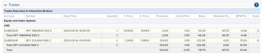
We closed by buying back the March contract at $0 02 x 100 = $2 making a realized profit of $40.70 after deducting commissions.

Next, we sold a new June contract at $1.24 x 100 = $124, thereby collecting a premium of $122.95 after deducting comission.

Portfolio Review

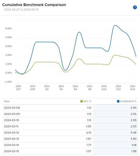
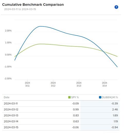
This week marked another period of losses for both the broader market and our portfolio, with our performance falling behind the market for the second consecutive week, partly due to the slight leverage from our options positions

Nonetheless, since its inception, our portfolio has managed to outperform the market by nearly 1%.

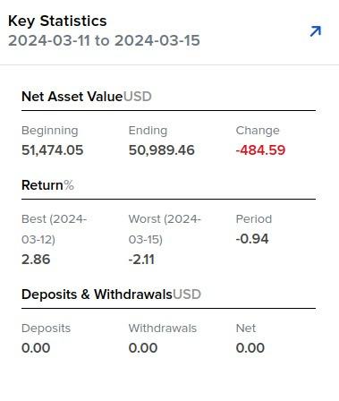
Initially, our portfolio experienced a decline leading up to the CPI report. Despite the CPI report coming in hotter than expected (refer to the Market Recap section for details), the market managed to rally on Tuesday. However, it faced downward pressure both before and after the release of a disappointing PPI report, continuing its descent into the close on Friday

We anticipate greater market volatility in the upcoming week, largely due to the scheduled FOMC meeting

Current Week:

Market Recap

On Tuesday, despite unexpectedly high consumer price index (CPI) inflation data, stocks managed to close with gains. The yield on Treasury bonds also increased, with the 2-year yield jumping by 0.06 percentage points to 4.59% and the 10-year yield by the same margin to 4.15%. The U.S. CPI for February showed a year-over-year increase of 3 2%, slightly above the previous 3 1% and exceeding the forecasted 3 1% rise The month-over-month figure for the headline CPI was 0 4%, aligning with expectations

However, the core CPI, which excludes food and energy prices, went up by 3 8% year-over-year, slightly down from January's 3.9% but still above the expected 3.7% increase.

This month-over-month, the core CPI increased by 0 4%, surpassing the 0 3% rise forecasted This continued trend of higher-than-expected CPI inflation could introduce some uncertainty regarding when the Federal Reserve might cut interest rates.

The stock market had a mixed performance on Wednesday following Tuesday’s rally, with the Dow Jones inching up and the Nasdaq falling Investors are now awaiting Thursday morning's release of the February U.S. producer price index (PPI) inflation and retail sales data. Meanwhile, the yields on Treasury bonds kept ticking upwards, with the 10-year note reaching around 4 19%

Thursday saw stocks closing lower while government bond yields climbed after U S producer prices and retail sales figures came in stronger than anticipated. The energy sector saw notable gains, fueled by a surge in oil prices, with WTI crude exceeding $80 for the first time in four months The headline PPI for February showed a 0 6% increase from the previous month and a 1 6% rise year-over-year, indicating a rebound in energy prices The core PPI, excluding food and energy, also saw a month-over-month increase of 0.3%, maintaining a steady annual growth of 2%. These inflation reports suggest the Federal Reserve might maintain a cautious stance on rate cuts, a topic likely to be emphasized in the upcoming FOMC meeting and its projections

Despite earlier market predictions of six rate cuts this year, expectations have now adjusted to align with the Fed's and our December projections of three cuts, hinting at the first reduction possibly occurring in June

U.S. retail sales in February bounced back from a slump in January, attributed to winter storms, though the increase was more modest than expected A boost in car sales and gas prices helped retail sales rise by 0 6% from the previous month

On Friday, the equity markets generally ended on a lower note, with the S&P 500 falling nearly 0.7% and the NASDAQ, known for its technological stocks, dropping around 1% In contrast, small-cap stocks showed better performance, as evidenced by the Russell 2000 Index, which rose approximately 0 4% Meanwhile, Treasury yields experienced a slight increase, with the 10-year yield closing slightly over 4.3% and the 2-year yield ending the day at about 4.74%.

Economic Data Preview

Following the release of the February CPI and PPI report, attention shifts to the upcoming FOMC meeting next week. Market expectations are for the Fed to hold rates steady at 5 25% - 5 50%

Key Takeaways:

Unexpectedly High CPI: On Tuesday, stocks closed higher despite a consumer price index (CPI) report showing inflation at 3 2% year-over-year for February, slightly above forecasts and the previous month's figure. The core CPI also rose more than expected, fueling speculation about the Federal Reserve's rate cut timeline

Mixed Stock Market Responses: The week saw fluctuating stock performances, with gains on Tuesday offset by mixed results on Wednesday and declines on Thursday and Friday Notably, the energy sector benefited from rising oil prices, with WTI crude topping $80 for the first time in months.

Inflation and Retail Sales Data: February's producer price index (PPI) and retail sales data came in stronger than anticipated. The PPI indicated a rebound in energy prices, and a modest increase in retail sales was supported by higher car sales and gas prices

Government Bond Yields Rise: Treasury yields increased throughout the week, reflecting the market's reaction to economic reports and adjusting expectations for the Federal Reserve's interest rate decisions

Federal Reserve's Rate Cut Projections: Despite initial market predictions of six rate cuts this year, stronger-than-expected inflation data has led to a reassessment Now, market expectations more closely align with the Fed's and our December projections of three cuts, with the first potential reduction in June

Friday's Market Close: The week concluded with equity markets mostly lower, small-cap stocks outperforming, and a slight increase in Treasury yields

Next week, we ' re set to delve into the Diagonal Call Spread, completing our overview of the two different type of spreads we utilized on trade initiation date. Following this, we'll have the tools needed to analyze the maximum potential profit and loss stemming from the day of trade initiation and compare this with how our portfolio has performed overall. Stay tuned!

Best regards,

JasonInvesting.com Team