Carbon Emission Forecasting using ARIMA

International Research Journal of Engineering and Technology (IRJET) e-ISSN:2395-0056

Volume: 09 Issue: 09 | Sep 2022 www.irjet.net p-ISSN:2395-0072

Carbon Emission Forecasting using ARIMA

Anshumaan Phukan 1 , Varad Vinayak Godse 2

1 Dept. of Computer Science Engineering, Bennett University, Greater Noida, Uttar Pradesh, India

2 Dept. of Computer Science Engineering, Bennett University, Greater Noida, Uttar Pradesh, India ***

Abstract - Global warming has become a growing concern in recent times. The root cause of the problem directs toward carbon emissions in the form of greenhouse gas.Theincreasinghumanactivitiesintervene intheearth's natural carbon-absorbing capacity. It leads to unwanted situations like the melting of ice caps, increasing sea levels, extreme weather conditions, and many others. The contributors to carbon emissions vary across industries ranging from electricity and heat production, transportation, agriculture, forestry, fossil fuel, and many more.

The idea behind our project is to run a prediction, analysis, and forecasting system over datasets related to carbon emissions. We will focus on certain core factors causing carbon emissions. It would include trends over the years, maximum and minimum contributors, etc. The analysis can be a foundation for predicting the future trends of these contributors.

1.INTRODUCTION

1.1 PROBLEM AND MOTIVATION

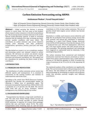
The distribution of carbon emissions across sectors has different aspects and consequences. It is essential to concentrate on the existing numbers and statistics to understandthescaleoftheissue.

According to the article from World Resources Institute, agriculture has become the second-largest emitter by releasing 6 billion tons of greenhouse gases. The emissionsincreasedby8percentfrom1990to2010,with a projection of a 15 percent rise till 2030. The sources range from fuel use on farms, fertilizers, manure management,urea,fieldburningofcropresidue.

1.2 BACKGROUND KNOWLEDGE

Transportation has become a large-scale contributor as well. The data from Oxford Martin School account for transportation for around one-fifth of carbon dioxide (CO2) emissions. A majority of it comes from passenger vehicles like cars, and buses- about 45.1%. The entire transportation sector involving road, air, and rail travel

contributes to 21% of total carbon emissions. The use of gasoline (fossil fuel) engines across vehicles has become therootcause.

Electricity is a widely used resource across industries and daily life. Its production from primary energy sources like coal, uranium, and natural gas contributes to emissions. According to a report from Planete Energy, electricity forms42.5%ofCO2emissions.Fromthistheamount,41% is produced from coal, 16% from hydropower, 22% from gas, 11% from nuclear power, and 10% percent from oil and renewables. The growing population and technology have triggered an exponential need for electricity. It has causedgrowingconcerns.

The carbon emissions from commercial and residential construction materials have become prominent as well. A report from nature communications sees a rapid emission increase of 750 Mt(22% globally) in 2020. It predicts the range of emissions to be 3.5 to 4.6 Gt in the upcoming 30 years.

Thestatisticalnumbersofthecontributorsaresignificantly large.Thecurrentscenariohintsatthegrowingconcernsof the future. The idea behind our effort will be to use the latesttechnologyfordevelopingananalysisandprediction model that provides concrete insights over different contributors.

Fig.1. Topindustriesresponsibleforemissions

International Research Journal of Engineering and Technology (IRJET) e-ISSN:2395-0056

Volume: 09 Issue: 09 | Sep 2022 www.irjet.net p-ISSN:2395-0072

Asseeninthescantotheright,thepatienthasabnormal tissue in the brain, which can be spotted as a white highlight towards the center of the scan. Unique patterns such as these can be used to detect any malignant in the brain, further helping us classify whether the brain is abnormal.

2. RELATED WORK

CO2 emissions is a big problem all around the planet. There are numerous studies begin conducted to reduce the CO2 emissions. There is an urgent need for a system that can estimate CO2 emissions and allow us to take appropriate actions to minimise the CO2 emissions. IN ordertosolvethisproblemmachinelearningcanbeused. The process of creating algorithms which can improve through experience is known as machine learning. For example, training a model which could automatically recognise fraud mails. Some models for prediction of CO2 emissionshavebeencreatedemployingmachinelearning.

In 2015 Researcher Chairul Saleh created a model which predictedtheCO2emissionsthatmakeuseoftheSupport Vector Machine algorithm in machine learning. Coal combustion and electrical energy were the input parametersforthemodel,bothofwhichplayamajorrole inCO2emissions.Inordertoevaluateandtrainthemodel, thedatafromtheAlcoholindustrywasobtained.InMayof 2017,anotherteamofresearchersdevelopedamodelthat described the quantity of CO2 released during the manufacturing of raw milk. Data from various milk manufacturing processes such as dairy processing and packaging waste disposal were provided to the model for predictionsofCO2 emissions.Accordingtothefindings of the research, 1120 g CO2 is released per litre in manufacturingofrawmilkproducts.

3.SYNOPSIS OF DATA

Thetrendsincarbonemissionsdependoncertainbaseline corefactorsthatcauselargerimpacts.

Thecorefactorsvaryasbelow-

1)CoalSector(CO2Emissions)

2)NaturalGasSectorCO2Emissions

3)Distillate Fuel, Including Kerosene-Type Jet Fuel, Oil SectorCO2Emissions

4)PetroleumCoke SectorCO2Emissions

5)ResidualFuelOilSectorCO2Emissions

6)PetroleumSectorCO2Emissions

7)GeothermalEnergySectorCO2Emissions

8)Non-BiomassWasteSectorCO2Emissions

9)Total

EnergySectorCO2Emissions

The use of coal across various industries grew to 45 % globally between 2001 and 2010. The burning of coal to generate steams to run turbines for electricity, as a raw material for agricultural fertilizers, as core material for cement production in constructions, as a combustion sourceinrailwayandwatertransportmadeitaprominent sourceofcarbonemissions.

It is responsible for 46% of global carbon emissions and 72%oftotalGreenHouseGas(GHG)emissions.

The emissions from natural gas are comparatively low but account for around half of what is caused by coal. A widescale use for generating electricity(steam generation units), fuel for transport (Compressed Natural Gas- CNG), heat for buildings, household use(refrigerator cooling), agricultureinputs(Pesticides,fertilizers,irrigation-cheaper than electricity) has caused a 43 percent increase since 2005. Although it contributes less compared to coal, it requiressignificantattention.

Distillatefuelsarefractionsofpetroleumformedasaresult of distillation subdues. It includes diesel fuels, jet fuel, and fuel oil(marine fuel, furnace oil, heavy oil). In 2021, the sector emitted 81.92 metric tons of carbon. It causes emissions almost four times that of petroleum. The recent days witnessedlimiteduse ofdiesel vehicles(notincluding heavy vehicles) and purer alternatives for jet and marine fuels.

Petroleum coke is a carbon-rich by-product of crude oil refining. Its use in the aluminum industry, graphite electrodes for the steel industry, and fuel for cement kilns has caused growing concerns. It emits more greenhouse gases and air pollutants than raw coal. China initiated the early use, with an 18.9 percent rise between 2010-and 2016. The economic advantages of petroleum coke benefit manyindustriesacrosstheglobe.

Petroleum is a widely used resource across industries and daily lives. A largescale application as fuel for vehicles extends to ammonia for fertilizers, heating furnaces, petrochemical industry, and Lubricants. It also produces manyharmfulby-products.Thesectoremitted1.22million metric tons of carbon dioxide in 2013. In 2020, a 6.3 percent decline in emissions marked the growth rate over thedecade.

International Research Journal of Engineering

and

Technology (IRJET) e-ISSN:2395-0056

Volume: 09 Issue: 09 | Sep 2022 www.irjet.net p-ISSN:2395-0072

Geothermal energy uses heat from the earth's core by producing minimal waste products. It emits 38 grams of Carbon dioxide per kilowatt of electricity produced. The minimal emissions from the sector introduce the need to monitortoavoidoverexploitation.

Non-biomass sectors like nuclear energy produce zero carbonemissions,buttheproductionprocesses(extraction andtransportofuranium,nuclearwastegeneration)cause harmfuleffects.

4.INTRODUCTION

Approach

We plan to achieve our goal by using a combination of machine learning and neural networks to forecast carbon emissionsbasedonmeaningfuldata.

Hypothesis testing would play a prominent role in our data analysis section. Hypothesis testing is a type of statistical method of drawing conclusions about a probability distribution or population parameter using data from a designated sample. It would be useful for our scenario because it allows us to evaluate 2 mutual exclusive statements, create an assumption and perform statistical analysis to reject or accept the hypothesis. In ourusecase,testssuchastheChi-Squaretest,T-Test,and AnnovaTestwillbeused.Thenullhypothesis,abbreviated as H0, would be our assumption. If statistical testing rejects our null hypothesis, we will define an alternate hypothesis. As a result, we can clearly deduce the relationships between individual carbon emission variables and total emission levels using these methodologies.

After understanding our data, the necessary feature engineering and selection procedures would be followed to ensure our model can predict carbon emissions with maximum accuracy. Techniques like mutual info index, correlation matrix, and variance threshold would play a huge role in selecting features that affect our prediction the most. Taking too many useful features can also result in a dimensionality curse. Feature extraction techniques like principal component analysis could help us in reducing dimensions by creating eigenvalues and eigenvectors. After acquiring the preprocessed data, numerous statistical models and neural networks will be trainedonit.Thisstudywillemploymodelssuchaslinear regression, polynomial regression, locally weighted regression, KNN, naive Bayes, SVM with different kernels, ensemble approaches with different base learners, and ANN. The base machine learning models like regression

The data is from the US Energy Information Administration,anditisatimeseriesdatathatspansfrom January1973toJuly2016.Itisacomprehensivecollection of carbon emission values spanning several years and involvesvariousenergysectorssuchasgeothermalenergy, naturalgas,petroleumcoke,andsoon.Withtheuseofsuch data throughout constant time intervals, we may run carbon emission forecasting models like ARIMA. It would beusefulincaseswhenvitaldecisionsmustbemadebased onpredictedemissionvalues.

will be our introductory approach, which would be followed by theimplementationofadvanced techniques.If the scatter plot portrays clear subdivisions among our dataset, models like KNN and SVM would be our first priority. Bagging and boosting ensemble techniques like decision tree, AdaBoost, gradient boost, and xgboost will help us combine several base models to produce one optimal predictive model. These techniques are also called as free lunch model as no single model wins. The aim of ensemblemodelsistobuildstronglearningbasedonweak learners.

The final model would be the custom neural network with differentexperimentaloptimizers,activationfunctions,and weight initialization techniques. Finally, we will perform a detailedinvestigationofourfindingsanddiscoveriesusing visualizationsandhyperparametertuningtodeterminethe parameters and model combinations that will provide the bestforecast.

5.PROPOSED METHODOLGY

The dataset consists of time-series data points collected atconstanttimeintervals.Thetime-dependentordynamic natureoftheproblemrequirestime-seriesmodeling.Itisa powerfultoolforextractingcurrentdataandmakingfuture predictionsandforecasting.

The overview of the steps for the final output involves the retrieval of the CSV time-series data, transforming or preprocessing of the data for suitable input, visualizing the data, applying different methods for testing whether it is stationary, transforming time-series data to stationary, finding optimal parameters to build SARIMA model, diagnosing,andvalidatingthepredictionsandforecasting.

RETRIEVAL

The read_csv function of pandas extracts the data in the form of a data frame. The info() function provides specifications describing 5096 observations with six columns. The data type of four columns is an object, while two have an integer. The current data frame does not

International Research Journal of Engineering and Technology (IRJET)

e-ISSN:2395-0056

represent a time series. The read_csv function needs specializedargumentstobringthedataintheformoftime series.Theargumentsgoasfollows-



parse_dates: Identifies the key for the date-time column. The initial dates come in string format. Forexample'YYYYMM'

DICKY-FULLER TEST

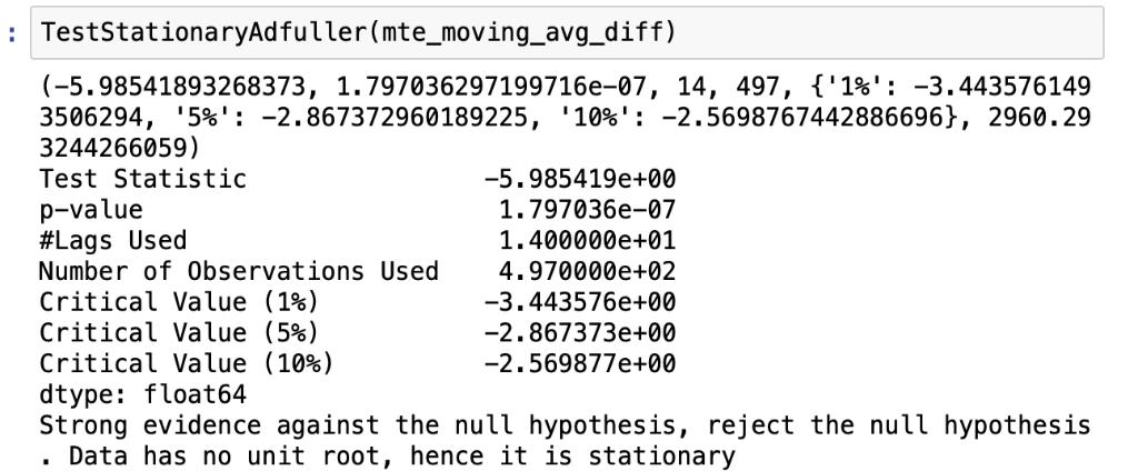
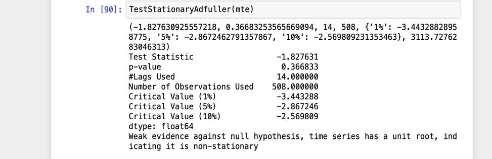
The test considers a null hypothesis. In this case, the null hypothesis is- that the time series is nonstationary. A Test statistic gets compared with critical values at different confidencevalues.IfthecriticalvalueexceedstheStatistic, the null hypothesis gets rejected. The time series is stationary.



index_col: Shifts DateTime column into index column.



date_parser: Converts an input string into a DateTimevariable.

Further pre-processing involves dropping null rows and null values in the index column using functions like notNull() and dropNa(). The coerce property with setting errors converts columns to float and fills problematic entries with Null(NaN). The to_numeric function converts theemissionvaluecolumnfromobjecttonumeric.

ANAYLYSIS

TEST STATIONARY

The dataset is analyzed to observe any trends and seasonality. The presence makes it nonstationary data. The removal of nonstationary elements converts the dataset into stationary. The residuals from the process formthebaseforfurtheranalysis.

Stationary Process- Astationaryprocesshasa probability distribution that remains unchanged with time. The parameters like mean and variance do not change over time.

The most common violation of stationarity comes from trendsinmean.Ifthecauseofnon-stationarityistheunit root, then it is not mean-reverting. If it is a deterministic trend,itcantransformtostationarity.

The analysis occurs with a single category of Natural gas CO2emissions.Thesamestepscanrepeatforothers.

The group-by function creates data frames with columns corresponding to the categories and having emission values.Theindexcolumnhasdate-timeentries.

GRAPH METHOD

TheplotmethodfromMatPlotlibgeneratesagraph.Ithas emissionvaluesonthey-axisandDateTime(inyears)data onthex-axis.Thestructureandtrendsoftheplotcanhelp toobservestationarity.

The opposite case accepts the null hypothesis keeping the time-seriesdatanon-stationary.

The Adler function from python takes the data and lag parameters. A lag describes the delay time between two sets of observations. Methods like Akaike Information Criterion(AIC) determine the optimal number of lags. The autolagparameterssetthenumberoflagstominimizethe AIC.

The test provides a p-value which gets compared to the user-providedcutoff.

It also gives a test statistic that compares critical values at differentconfidencelevels.

CONVERSION TO STATIONARY

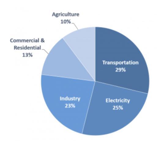
The technique focuses on taking the mean of a set of consecutivevalues.

We target a yearly trend that requires an average of 12 consecutive values or months. The value in each entry in thecolumnisthemeanoftheprevious12values.Thefirst 11 values remain null as they do not have a sufficient number of values prior(12). The original data gets subtractedfromthenewdataofthemovingaverage.Itgets tested through the dicky fuller test that tells whether the conversiontostationarityissuccessful.

Thetechniqueusestherollingmethodfrompython.

Adding seasonal terms to an ARIMA model results in a model called SARIMA. This model is characterized by 3 terms:

P:orderoftheautoregressiveterm

Q:orderofmovingaverageterm

Volume: 09 Issue: 09 | Sep 2022 www.irjet.net p-ISSN:2395-0072 © 2022, IRJET | Impact Factor value: 7.529 | ISO 9001:2008 Certified Journal | Page1313

D: number of differencing required to convert non stationarytimeseriesdatato stationary.

Whena seasonal ARIMAmodel needstobefitted,ourgoal shouldbetodeterminetheparametersthatareresponsible for optimizing the metric of interest. While implementing

International Research Journal of Engineering and Technology (IRJET) e-ISSN:2395-0056

Volume: 09 Issue: 09 | Sep 2022 www.irjet.net p-ISSN:2395-0072

seasonal ARIMA, we considered two possible scenarios. First one being a stationary time series data with no dependence.Inthiscase,residualsweremodeledaswhite noise. The second case would involve a time series data withnoticeabledependenceamongvalues.Wespecifically needed to implement statistical model like ARIMA in the secondscenario.

For forecasting stationary time series data, the ARIMA model,whichisalinearfunctionakintolinearregression, iscommonlyutilized.

For finding optimal parameters, we implemented two major techniques: Plotting of ACF and PACF curve. Autocorrelation Function and Partial Autocorrelation Function are both responsible for measuring correlation betweents(timeseries)withalaggedversionofitself.But in the case of PACF, elimination of variations are already explained beforehand by intervening comparisons. As a result, these two graphs will be used to determine the model'stuningparameters(pandq).

Second method involves Grid Search for optimizing parameters. This method was included as it a more systematic approach compared to the previous one. It is an iterative technique of exploring all possible combination of parameters of our forecasting model. Seasonal ARIMA model will be fitted all combinations. After exploration, parameters that yield the best performance will be opted. A function called SARIMAX() was used in our case to perform hyperparameter optimization.

6.RESULTS

STATIONARITY

Theresultofthefirstadderfullertestyieldedagreaterval ueof -1.827631forTestStaticcomparedtothecriticalval ues at different confidence levels. The initial critical value wassetat0.01.Theconfidencelevelsweresetat95,90%, 99%.Itmeans5%(-2.867303),10%(-2.569840)and1%( -3.443418)ofthecriticalvalue.

Themovingaveragemethodresultsinteststatic(-5.98541 9e+00)lesserthancriticalvalues10%(-2.569840),1%(-3. 443418)and5%(-2.867303)

EVALUATION

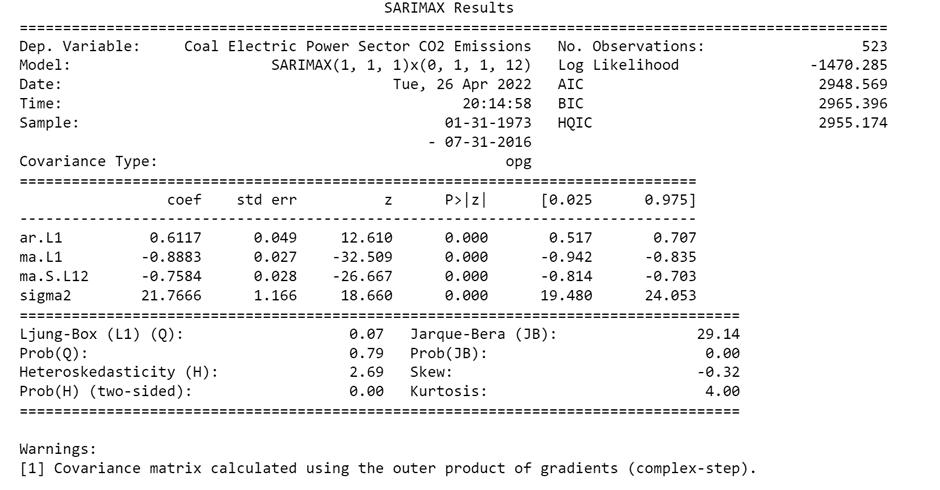
For performing evaluation, we first plotted the Autocorrelation Function (ACF) and Partial Autocorrelation Function (PACF) curve for our seasonal ARIMAmodel.Asfindingtheoptimalparametersmanually graphs is time consuming, we opted for grid search method. Using this method, we explored each and every possible combination of parameters possible. When analyzing and comparing statistical models with various parameters, each can be rated against the others based on how well they fit the data or their ability to properly forecast future data points. A statistical value called AIC was used for the scenario. For this example, weare taking emission values only for Coal Electric Power Sector. The Akaike Information Criterion value measures how well a model fits our training data. It is calculated using the number of independent variables, and the maximum likelihoodestimateofthemodel.AICvaluesareonlyuseful incomparisonscenarios.AlowerscoreofAICindicatesour model is performing well. After performing hyperparameter tuning through grid search, the SARIMAX

International Research Journal of Engineering and Technology (IRJET) e-ISSN:2395-0056

Volume: 09 Issue: 09 | Sep 2022 www.irjet.net p-ISSN:2395-0072

(1, 1, 1)x(0, 1, 1, 12) yielded the lowest AIC score of 2003.553. Hence, we considered these conditions for our proposed model. Next step we went for in-depth analysis ofthemodelwiththeabove-mentionedparameters

Fig:State-spacemodelresultforCoalElectricPower Sector

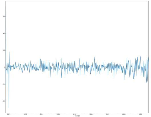
The next analysis would plot the residual errors for our seasonalARIMAmodel.

Fig:DiagnosticPlot

TheredKDElineinthetoprightplotcloselyresemblesthe N(0,1) line. This indicates the residual residuals are normally distributed. However, we can observe some deviations in the straight line, indicating the normal distribution is not perfect for the distribution of errors in the forecast, but it is defiantly acceptable. The qq-plot at the bottom left again indicated our residuals are normally distributed.

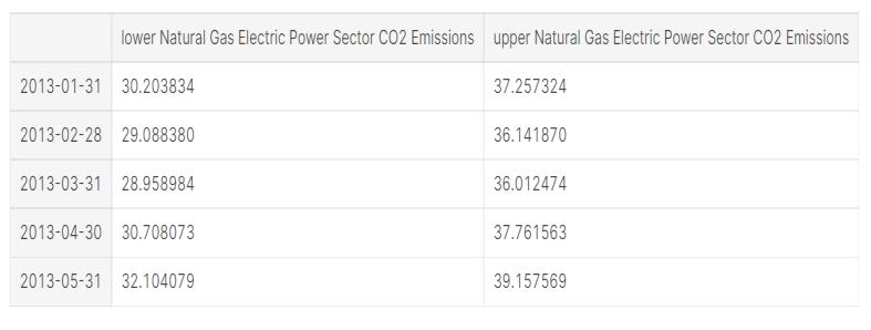
Afterweobtainedourmodelfortimeseriesforecasting,we startedcomparingthepredictedandrealvaluesofthedata. We got the values and accompanying confidence intervals for time series forecasts using the get prediction() and conf_int()properties.

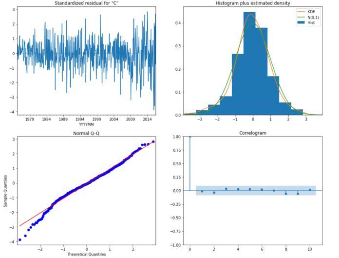
Fig:ResidualerrorsforSARIMAforcoalpowergeneration

Theresidualerrordistributionisdepictedinthediagram. Itshowsthatthepredictionisalittleskewed.

Fig:Onestepaheadforecast

The table above portrays one-step forecasts at each point usingtheentirehistoricaldatauntilthecurrentpoint.

International Research Journal of Engineering and Technology (IRJET) e-ISSN:2395-0056

Volume: 09 Issue: 09 | Sep 2022 www.irjet.net p-ISSN:2395-0072

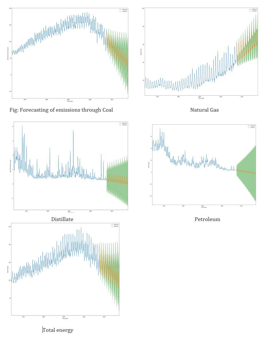
Itconsistsofvariationsintheforecastedline.

Thetotalenergyplotcombiningeverysectorshowsadown wardtrendwithnegligiblevariations.

7.CONCLUSION

Thecategorieslikenaturalgasandcoalareusedwidelyan dhaveledtoenvironmentalconsequences.Thegrowingtre ndinnaturalgasisalarming,butadecreasingtrendincoal highlightsanimprovedscenario.

Othercategorieslikepetroleumanddistillatehave constantgrowth.

Fig:RealvsForecastedvaluesofCO2emissionsforcoal powergeneration

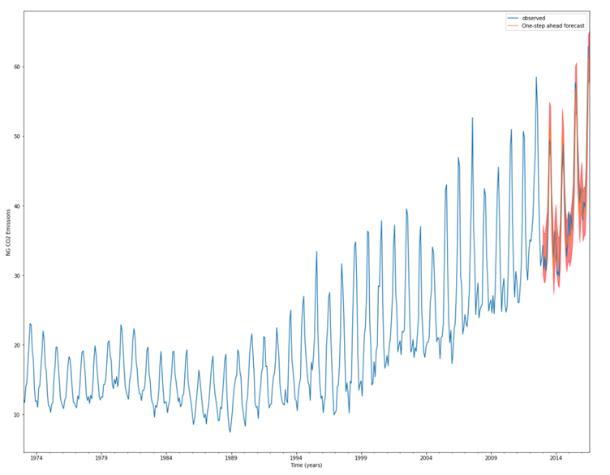
Overall, our forecasts closely match the true numbers, indicatingasimilarpatternofbehavior.

ThemodelwebuiltgaveusanMSEscoreof14.39andan RMSEscoreof3.7936,whichisfairlylow.Themodel'spur pose was to achieve high-quality predictive power throug hdynamicforecasting.

FORECASTING

Theget_forecastmethodundertakesthetotalnumberofst epstoforecast.Theconf_init()methodprovidesconfidenc eintervals.Aconfidenceintervalhasasetofvalueswithi nwhichtheparametercanlie.

Thedatafromtheabovefunctionisusedtodrawtheplots todisplaytheforecastfordifferentcategories.

Thehighlightedareaingreencolorrepresentstheotherp ossiblevariationsintheforecastedvalues.Theforecasting modelperformsbetterwhenitisless.

Thenaturalgasforecastshowsanupwardtrendforthene xttenyears.Thegreenarearemainsshorterasaresultof agoodprediction.

Thecoalforecastshowsadownwardtrendhighlightingth edecreaseduseofcoalinthefuture.Theshortergreenare acorrespondstoagoodprediction.

Thedistillatefuelcategorywitnessesaslightlydecreasing butalmostconstanttrend. Thelargergreenarea suggests morevariationsintheforecastedline.

Thepetroleumcategorywitnessesa slightlydecreasing tr end.

Thepatternsandtrendsforecastedbythemodelproveess entialasithelpstounderstandthefuture.Theglobalaimof achievingnetcarbonemissiontozeroby2050needsconti nuous analysis and predictions over the current scenarios. Thecurrentemissiontrendmightseemconstantordecrea sing, but the situation will deteriorate because the present emissionshaveeffectsinthefarfuture.Hypothetically,ifw ereducethenetemissionstozeroatonce,theimpactofrec entemissionswilltriggertheproblemagain.

Theuseoftechnologytoanalyzedatasetsforgeneratingins ightsplaysasignificantrole.Thevariousmachinelearning techniques extended by python libraries help run efficient andusefulpredictionsandforecasts.

Wefocussedonthetechniquestogenerateaforecastingan alysis that is useful to environmentalists, researchers, and othersworkingtowardsthecause.

International Research Journal of Engineering and Technology

(IRJET)

e-ISSN:2395-0056

Volume: 09 Issue: 09 | Sep 2022 www.irjet.net p-ISSN:2395-0072

https://www.machinelearningplus.com/timeseries/augmented-dickey-fuller-test/ 

https://machinelearningmastery.com/moving -average-smoothing-for-time-seriesforecasting-python/ 

https://neptune.ai/blog/select-model-fortime-series-prediction-task 

https://towardsdatascience.com/identifyingar-and-ma-terms-using-acf-and-pacf-plots-intime-series-forecastingccb9fd073db8?gi=e940575f86f8 

https://www.yourdatateacher.com/2021/05/ 19/hyperparameter-tuning-grid-search-andrandom-search/ 

https://robert-alvarez.github.io/2018-06-04diagnostic_plots/ 

https://pandas.pydata.org/docs/reference/api /pandas.read_csv.html

REFERENCES

https://www.wri.org/insights/4-chartsexplain-greenhouse-gas-emissions-countriesand-sectors 

http://www.annualreviews.org/doi/abs/10.1 146/annurev-environ-032310-112100 

https://www.planeteenergies.com/en/medias/close/electricitygeneration-and-related-co2-emissions 

https://machinelearningmastery.com/arimafor-time-series-forecasting-with-python/