Comparative Analysis of Tuning Hyperparameters in Policy-Based DRL Algorithm for Self-Driving Scenar

International Research Journal of Engineering and Technology (IRJET) e-ISSN: 2395-0056 Volume:09Issue:08|Aug2022 www.irjet.net p-ISSN: 2395-0072

Comparative Analysis of Tuning Hyperparameters in Policy-Based DRL Algorithm for Self-Driving Scenario

1Tribhuvan University, Institute of Engineering, Pulchowk Campus, Lalitpur, Nepal -*** -

Abstract: This technical article makes a comparative study on the outcome of policy-based deep reinforcement learning algorithm PPO (Proximal Policy Optimization) at different hyperparameter values in self driving scenario to analyze its effectiveness in navigation of vehicles. The agents are trained and evaluated in OpenAI Gym CarRacing-v0 simulation environment. The action space is continuous and the observation spaces are images of 96x96x3 dimension which is fed to the actor-critic network architecture. Three major hyperparameters discount factor, clip range and learning rate are altered to evaluatetheirperformanceingivenenvironment.Thebehaviorsoftheagentswhiletuningthehyperparametersareobservedand analyzed against evaluation metrics such as mean episode reward, policy loss, value loss, etc. The agents were found to perform optimallyatthediscountfactorof0.99,cliprangeof0.2andlearningrateof0.0003whicharealsothebaselinedefaultvalues.

Key Words: PPO,DRL,ProximalPolicyOptimization,DeepReinforcementLearning,SelfDriving

1. INTRODUCTION

Deep reinforcement learning has prevailed in recent times as a popular algorithm to solve navigation problem for autonomous vehicles. It is seen as the possible tool to replace classical control mechanisms used in autonomous systems with numerous sensors and their compute hardware and software stack by simple output oriented programminglogic.

Various types of learning agents have been developed over the years to accomplish multitude of tasks among which model-based algorithms, value-based algorithms and policy optimizing algorithms are popular among researchers. Model based algorithms represent the system in a dynamic model form and tries to optimize the solution. Value based algorithmsprepareatableofvalueforeachstate-actionpair which represents the possible outcome of the agent incorporating the reward value for upcoming outcomes. Policy optimization algorithms guides the agent directly depending upon whether the policy is deterministic or stochastic to maximize the reward based upon the probability distribution of outcomes developed and optimized previously during the training. In this article, we will compare and analyze the performance of Proximal

Policy Optimization algorithm to evaluate its navigation efficiencyinselfdrivingscenario.Theoutcomesareweighed up in terms of evaluation metrics such as mean episode reward,policyloss,valueloss,etc.

2. RELATED WORKS

The deep learning revolution started at around 2012 as function approximators in various domains which led researchers to investigate the implementation of these neural networks in pre-existing reinforcement learning algorithms. The new approach started using images as the state of the agent instead of position, velocity and distance tocollisionwithotherobstaclesinthesurrounding.DeepQNetwork (DQN) was introduced as a potential solution to solve high-dimensional state space environment with policies that worked efficiently in large array of problems with same algorithm, network architecture and hyperparameters [1]. The DQN agent succeeded in multiple Atari games with pixel and game score as inputs and performed better than majority of algorithms previously proposed, which were effective only in domains with fully defined,lowdimensionalstatespace.WhileDQNcouldsolve problems with discrete action spaces quite effectively, a widerangeofrealphysicalenvironmentsaremuchcomplex

International Research Journal of Engineering and Technology (IRJET)

e-ISSN: 2395-0056

Volume:09Issue:08|Aug2022 www.irjet.net p-ISSN: 2395-0072

and consists of tasks requiring continuous control. Deterministic policy gradient (DPG) algorithms were developed to encounter the problems with continuous action spaces [2]. REINFORCE was one of the early straight forward policy-based algorithms which operated by converging in the direction of performance gradient and hence, separate network for policy evaluation was not trained[3].

Deep Deterministic Policy Gradient (DDPG) was developed adapting to the underlying principles of DQN which could address the problems with continuous action domain [4] Actor-critic architecture was incorporated in the algorithm which could optimize its own policy based on the state values obtained from critic network. Trust region policy optimization (TRPO) was introduced which prevented the policies from deviating excessively on a single cycle by adding a surrogate objective function to the algorithm [5] Advantage Actor Critic (A2C) was put forward as synchronous version of Asynchronous Advantage Actor Critic (A3C) algorithm [6]. A2C has larger batch size which ensures the completion of training for each actor in that particular segment before the mean parameters are updated. Soft Actor Critic (SAC) is also a popular off-policy deepreinforcementlearningalgorithmbasedonmaximizing the entropy by actor to optimize expected reward through randomness[7].

Among the algorithms proposed, Proximal Policy Optimization (PPO) is prominently used in testing selfdriving features due to its effectiveness in the given scenario. The algorithm fine-tuned the outcome of previously existing policy-based reinforcement learning algorithms in which surrogate objective function is optimized using stochastic gradient ascent [8]. PPO allows multiple gradient updates over a data sample in minibatches with repeated epochs. The algorithm, when it first launched, outperformed other online policy gradient methods in tasks including simulated robotic locomotion andAtarigames.

Kiran et al. have outlined the development of deep reinforcement learning algorithms on autonomous driving scenario [9]. Chen et al. discussed and experimented with model free DRL algorithms for urban driving conditions

[10]. Deep reinforcement learning has been proposed as a solutionformaplessnavigation,andways to bridgethe gap between virtual and real environment was also addressed [11]. Apart of ground vehicles, DRLs have also been researched and utilized in the domain of unmanned aerial vehicles (UAV) and unmanned underwater vehicles (UUV) [12]

3. SIMULATION SETUP

Despite of reinforcement learning algorithms performing quite well in controlled environments with finite state spaces and pre-defined quantifiable goals, autonomous driving is much complex scenario, especially in real world applications.Thechallengesare evenhighergivenitssafety issues. Hence, the algorithms are tested and evaluated in oversimplified gaming or simulated environments to verify itsoutcome.

3.1 Environment

The algorithms, in this article, are tested and evaluated on OpenAI Gym CarRacing-v0 environment which is much simplified version for autonomous driving scenario. The environment does not contain any static or dynamic obstacles which makes the task much easier than what wouldbeexpectedinrealworldapplication.Stablebaseline algorithm provided by the platform is compared against agents with varied hyperparameter values. Each agent was trained for an approximate of 200,000 timesteps to obtain theresult

Fig - 1:OpenAIGymsampleracetrack

International Research Journal of Engineering and Technology (IRJET) e-ISSN: 2395-0056

Volume:09Issue:08|

3.2 Action/Observation Spaces

www.irjet.net p-ISSN: 2395-0072

statevaluedependinguponwhetheritisbeingusedbyactor orcritic.Thelossfunctionisgivenby:

The action space is continuous with steering value ranging from –1 to 1 for extreme left and right, and 0 for no movement. The gas amount can be increased or decreased within the range of 0 to 1 depending upon the amount of acceleration required. Similarly, braking range is within the value of 0 to 1 for no braking to full stop. The observation spaces are the images of 96x96x3 pixel size and color channels.

Lt CLIP+VF+S(θ)=Ê[Lt CLIP(θ)-c1Lt VF(θ)+c2S[πθ](st)]

Inaboveequation, Lt CLIP(θ)=Êt[min(rt(θ)Ât,clip(rt(θ),1-ɛ,1+ɛ)Ât)]

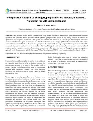
Also,the2nd and3rd termwithco-efficientc1andc2arethe mean squared error of value function and entropy loss respectively.The rt(θ) term isthe ratio of new policy to the oldpolicy.

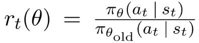
Fig - 2:Observationspacesample

3.3 Reward Functions

The racecar environment is considered solved when the agent consistently scores 900+ points. Given that the number of tiles visited is N, reward of +1000/N is granted foreverytracktilevisited.Also,0.1pointisreducedoneach frameencouragingthevehicletoreachthedesignatedscore pointfaster.Anepisodeiscompletedwhenallthetilesofthe trackarevisited.Ifthevehicleistoofarawayfromthetrack, 100 point is reduced which eventually terminates the episode.

3.4 Network Architecture

Proximal Policy Optimization (PPO) adopts actor critic architecture, and in case of stable baselines provided by OpenAI, the network consists of two separate parts. The feature extractor class uses Convolutional Neural Network (CNN) to extract useful information from the image and is sharedby bothactorandcritictoreducecomputationtime. Thefullyconnectednetworkmapsthefeaturestoactionsor

PPO limits the update to policy network by restricting this ratiotocertainvaluessothatthesuddenperformancedrop prevalentinactor-criticarchitectureisavoided.ThetermÂt is introduced to identify the good states and provide advantagetothesesates.Also,thelearningiterationsduring training is carried out over small fixed length trajectory of memoriesandmultiplenetworkupdatepersampleisdone

3.5 Hyperparameters

The default hyperparameters and arguments used by the baselinealgorithmaretabulatedbelow.

Table - 1: Defaulthyperparametervalues

Hyperparameters

Argument Default value

Learningrate learning_rate 0.0003

Numberofsteps n_steps 2048 Mini-batchsize batch_size 64

Numberofepochs n_epochs 10

Discountfactor gamma 0.99 Trade-offfactor(biasvs variance) gae_lambda 0.95

Clippingparameter clip_range 0.2

Entropyco-efficient ent_coef 0.0 Valuefunctioncoefficient vf_coef 0.5

Maximumgradient clippingvalue max_grad_norm 0.5

Verbositylevel verbose 0

International Research Journal of Engineering and Technology (IRJET) e-ISSN: 2395-0056 Volume:09Issue:08|Aug2022 www.irjet.net p-ISSN: 2395-0072

ThecodeiswrittenandexecutedonJupyterNotebookusing PyTorchframeworkwithnoGPUacceleration.

4. OBSERVATIONS AND DISCUSSIONS

The algorithms are compared and evaluated in terms of average reward per episode during training and evaluation cycles. Loss and time metrics are also analyzed to better understand the advantage and shortcomings of each algorithm.Threemajorhyperparametersi.e.discountfactor (γ), clip range and learning rate (α) are altered and their behavior over 200,000 timesteps are observed to analyze their performance. The results are visualized using tensorboardlogdataandgraphsprovidedbytheplatform.

4.1 Discount Factor

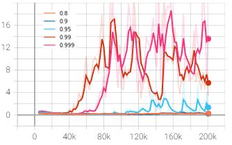
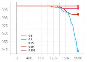
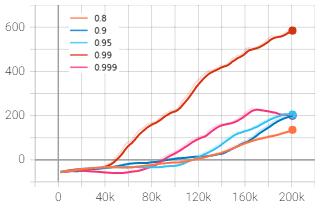
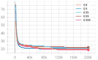
Thediscountfactoristhemeasureofhowmuchthepolicyis influencedbypossiblereturnfromfuturestepscomparedto the immediate reward. The discount factor was altered withintherangeof0.8to0.999andthegraphswereplotted inTensorboard.Inthefiguresbelow,orange,darkblue,light blue,redandpinkplotsrepresentthediscountfactorof0.8, 0.9, 0.95, 0.99 and 0.999 respectively. The rewards and lossesareplottediny-axisagainstthetimestepsinx-axis.

4.1.1 Graphs

ThegraphsobtainedfromtheTensorboadareshownbelow:

Chart – 2: Meanepisodelength(y)vs.timesteps(x)

Chart – 1: Meanepisodereward(y)vs.timesteps(x)

Chart – 3: Policygradientloss(y)vs.timesteps(x)

Chart – 4: Valueloss(y)vs.timesteps(x)

International Research Journal of Engineering and Technology (IRJET) e-ISSN: 2395-0056 Volume:09Issue:08|Aug2022 www.irjet.net p-ISSN: 2395-0072

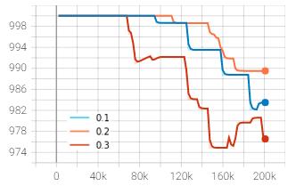
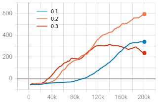
0.2 and 0.3 represented by blue, orange and red plots respectively.Theprogressionoftimestepsisplottedalongxaxisandtherewardsandlossesaremappediny-axis.

4.2.1 Graphs

ThegraphsobtainedfromtheTensorboadareshownbelow:

Chart – 5: Framepersecond(y)vs.timesteps(x)

4.1.2 Inference

The mean episode reward was found to be maximum at discountfactorof0.99asrepresentedbyredcurvewhichis also the baseline default value. The discount factor was increased and decreased to 0.999 and 0.95 which gave the mean reward of 202 and 204 respectively at 200,000 timesteps, which is much lesser than 594 points obtained from 0.99. The discount factor wasfurther decreased to 0.9 and0.8asrepresentedbydarkblueandorangecurvewhich further lowered the outcome to 200 and 135 respectively. Hence, it can be inferred from the experiments above that the discount factor of 0.99 is best suited among the tested valuesforthegivenenvironment.

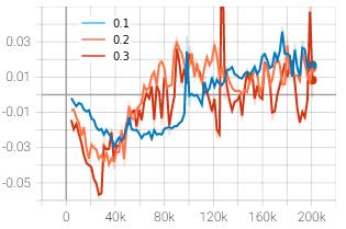
The policy gradient loss seemed to be gradually increasing initiallyin either direction oftheaxisand decreasing asthe timestep progressed. It can be expected from the pattern thatthecurvewillconvergetowardszeroneartheendifitis furthertrainedto1-2milliontimesteps.Thepolicylosswas higherinitiallybecausetheagenthadnotlearnedasmuchin the beginning, hence large policy update occurred in each iteration. However, the more the agent learned, the policy started becoming more stable resulting in lower loss per update.

4.2 Clip Range

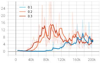
The restriction imposed on the ratio of new policy to old policy of the agent which determines the extent of update thata networkcanhaveperiterationisgivenbycliprange. Thealgorithmwastestedagainstthreecliprangevalues0.1,

Chart – 6: Meanepisodereward(y)vs.timesteps(x)

Chart – 7: Meanepisodelength(y)vs.timesteps(x)

International Research Journal of Engineering and Technology (IRJET) e-ISSN: 2395-0056 Volume:09Issue:08|Aug2022 www.irjet.net p-ISSN: 2395-0072

to a steady range once the agent stabilized. The orange and red curve representing the clip range of 0.2 and 0.3 respectivelystartedascendingataround30k-40ktimesteps and reached their peaks at about 100,000 timesteps. The curvesstarteddescendingandstabilizedaroundthevalueof 6. The blue curve with clip range of 0.1 started ascending muchlaterandmaygivebetterresultsathighertimestepsif trained for longer. However, at 200,000 mark, the loss was foundtobelowestforcliprangeof0.2withtheapproximate valueof3.5.

4.3 Learning Rate

Chart – 8: Policygradientloss(y)vs.timesteps(x)

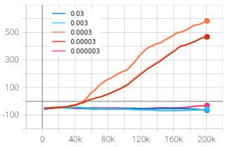
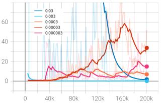
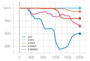
PPO performs mini-batch stochastic gradient ascent for updatingitsnetworkparameters,andlearningratecontrols the pace at which the updates take place. The baseline algorithm was tested against varying learning rate values rangingfrom0.03to0.000003toanalyzeitsinfluenceinthe agent’s overall performance. The learning rate values of 0.03, 0.003, 0.0003, 0.00003 and 0.000003 are depicted by dark blue, light blue, orange, red and pink respectively. As usual, x-axis represents timesteps and y-axis represents rewardsandlosses.

4.3.1 Graphs:

ThegraphsobtainedfromtheTensorboadareshownbelow:

Chart – 9: Valueloss(y)vs.timesteps(x)

4.2.2 Inference

Theaverageepisoderewardstartedincreasingfasterincase of clip range 0.3 represented by red curve, however, the growth was not steady and stopped increasing after about 120,000 timesteps. The blue curve representing the clip range of 0.1 started sloping up later than other curves and yet succeeded in overtaking the clip range of 0.3. The average episode reward of default agent with clip range of 0.2wasstillmaximumthanotheragentsatthelandmarkof 200,000 timesteps. The above experiment implies that tuning the clip range towards the lower value than the baseline default may produce better results than tuning it towardshighervalueifitistobedoneatall.

The value loss curves were as expected for PPO learning cycles.Thelossincreasedinitsearlycyclesandcamedown

Chart – 10: Meanepisodereward(y)vs.timesteps(x)

International Research Journal of Engineering and Technology (IRJET) e-ISSN: 2395-0056 Volume:09Issue:08|Aug2022 www.irjet.net p-ISSN: 2395-0072

4.3.2 Inference

Chart – 11: Meanepisodelength(y)vs.timesteps(x)

The mean episode reward of baseline algorithm with learning rate 0.0003 was found to be at an approximate of 590 points (unsmoothed value) after 200,000 timesteps as depictedbytheorangecurve.However,whileincreasingthe learning rate to 0.03, the mean episode reward came down to –65 points as shown by dark blue curve. Hence, the learning rate was further decreased to 0.00003 and the episode reward reached an average value of 470 points whichisstilllesserthanthatobtainedfrombaselinedefault. The learning rate was then increased one unit higher than thebaselinevalueto0.003whichalsogavesimilarresultas that of 0.03. On the last experiment, the learning rate was decreased to 0.000003, however, the algorithm didn’t converge at all leaving negative average reward. It can be inferred from the above experiments that the learning rate of0.0003 isoptimumamongthetestedvaluesforthegiven environment.

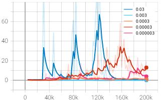
Incaseofthelossplot,aconsistentpatternwasobservedin thetotallossofagentwithlearningrateof0.03represented bydarkbluecurve.Thelossappearedtopeakupabruptlyat times taking much longer time to fall back to its previous range. This is possibly due to the performance falling of actor critic architecture which became prominent when the learningratewasnotrestrictedtosmallvalue.

Chart – 12: Totalloss(y)vs.timesteps(x)

5. CONCLUSION

Chart – 13: Valueloss(y)vs.timesteps(x)

It can be concluded from the above observations that the hyperparameters used by baseline algorithm as shown in Table 1 are optimized to give the best possible outcome in majority of scenarios. However, the data and graphs obtained were based on training carried out for 200,000 timestepswhichismuchlesstoinfertheagent’sbehaviorin longerrun.Inmajorityofcases,themeanepisoderewardis within 400-500 which is only half the expected reward for the racetrack to be considered completed. Hence, training the agent for longer timesteps i.e. an approximate of 1-2 millions could yield better insight into the performance of algorithm at different hyperparameter values. For future work, the baseline algorithm can be tweaked to fit in other tools and techniques such as image processing, altering

International Research Journal of Engineering and Technology (IRJET) e-ISSN: 2395-0056 Volume:09Issue:08|Aug2022 www.irjet.net p-ISSN: 2395-0072

framestacksand/ordiscretizingtheactionspacetoimprove performanceintermsoftrainingtimeandaccuracy.

REFERENCES

[1] Mnih, V., Kavukcuoglu, K., Silver, D., Rusu, A. A., Veness,J.,Bellemare,M.G.,...&Hassabis,D.(2015). Human-level control through deep reinforcement learning. nature, 518(7540),529-533.

[2] Silver,David&Lever,Guy&Heess,Nicolas&Degris, Thomas & Wierstra, Daan & Riedmiller, Martin. (2014). Deterministic Policy Gradient Algorithms. 31stInternationalConferenceonMachineLearning, ICML2014.

[3] Williams, R. J. (1992). Simple statistical gradientfollowing algorithms for connectionist reinforcementlearning. Machinelearning, 8(3),229256.

[4] Lillicrap, T. P., Hunt, J. J., Pritzel, A., Heess, N., Erez, T., Tassa, Y., ... & Wierstra, D. (2015). Continuous control with deep reinforcement learning. arXiv preprintarXiv:1509.02971.

[5] Schulman, J., Levine, S., Abbeel, P., Jordan, M., & Moritz, P. (2015, June). Trust region policy optimization. In International conference on machinelearning (pp.1889-1897).PMLR.

[6] Mnih, V., Badia,A. P.,Mirza, M., Graves, A., Lillicrap, T., Harley, T., ... & Kavukcuoglu, K. (2016, June). Asynchronous methods for deep reinforcement learning. In International conference on machine learning (pp.1928-1937).PMLR.

[7] Haarnoja,T.,Zhou,A.,Hartikainen,K.,Tucker,G.,Ha, S., Tan, J., ... & Levine, S. (2018). Soft actor-critic algorithms and applications. arXiv preprint arXiv:1812.05905

[8] Schulman, J., Wolski, F., Dhariwal, P., Radford, A., & Klimov, O. (2017). Proximal policy optimization algorithms. arXivpreprintarXiv:1707.06347

[9] Kiran, B. R., Sobh, I., Talpaert, V., Mannion, P., Al Sallab, A. A., Yogamani, S., & Pérez, P. (2021). Deep reinforcement learning for autonomous driving: A survey. IEEE Transactions on Intelligent TransportationSystems

[10] Chen, J., Yuan, B., & Tomizuka, M. (2019, October). Model-free deep reinforcement learning for urban

autonomous driving. In 2019 IEEE intelligent transportation systems conference (ITSC) (pp. 27652771).IEEE.

[11] Tai, L., Paolo, G., & Liu, M. (2017, September). Virtual-to-real deep reinforcement learning: Continuous control of mobile robots for mapless navigation. In 2017 IEEE/RSJ International Conference on Intelligent Robots and Systems (IROS) (pp.31-36).IEEE.

[12] Pham,H.X.,La,H.M.,Feil-Seifer,D.,&Nguyen,L.V. (2018). Autonomous UAV navigation using reinforcement learning. arXiv preprint arXiv:1801.05086.