EmmanuelEpau,LoganEadesandThomasZwiller
MendozaCollegeofBusiness,UniversityofNotreDame
MSBR-70320-SS-1F:TimeSeriesForecasting
ProfessorSriramSomanchi
February28th,2025
Data Description
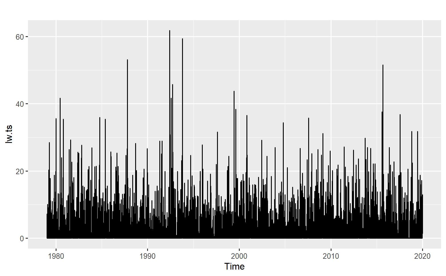
Our project utilized two data sources. The first dataset collected 15,341 daily observations of London weather1 . Each observation was comprised of ten (10) attributes dating from 1979 to 2020 and included the date of the observation, the cloud coverage, the amount of sunshine in hours, global radiation measurements, minimum and maximum temperature (in Celsius), the average temperature for the day (in Celsius), the pressure, depth of snow in centimeters, and lastly the amount of rain in millimeters. Our team found the dataset on Kaggle, which was initially created by reconciling measurements from requests for individual weather attributes provided by the European Climate Assessment (ECA). A weather station near Heathrow Airport in London, UK, recorded the measurements of this particular dataset.
The second dataset that the team used contained 3,510,433 observations on London energy consumption2 , with three attributes dating from 2011 to 2014. The observations contain a unique individual household identifier, the date, and the household's energy consumption in kWh. We found this dataset on Kaggle, which was initially created by aggregating hourly energy consumption data from individual London homes provided by UK Power Networks The dataset then keeps track of the energy consumption of 5,567 randomly selected households in London from November 2011 to February 2014. The energy consumption dataset was joined to the London Weather dataset via the date, enabling our team to observe the correlation between the date and electricity consumption as well as temperature and electricity consumption.
1 Werr, E F (2022, May 16) London Weather Data Kaggle https://www kaggle com/datasets/emmanuelfwerr/london-weather-data/data
2 Werr, E F (2022b, May 17) London Energy Data Kaggle https://www kaggle com/datasets/emmanuelfwerr/london-homes-energy-data
Questions Addressed
Historically, London has dealt with large-scale electrical blackouts. In 1974, a global oil crisis combined with a miner strike due to lagging wages resulted in the British government implementing a three-day working week (Roller, 2021) The main idea behind the three-day working week was to limit commercial electricity consumption to conserve the limited coal supply, allowing the government to ride out the miners' strike (Roller, 2021). However, the plan crippled the British economy, and after a snap election was called, the miners saw a raise in wages, and the three-day work week ended after three months. The three-day working week was not the only time London dealt with blackouts. On October 16, 1987, London experienced a storm with winds of up to 120 mph, which reportedly knocked out over “15 million trees [which] knock[ed] out powerlines and blocked the roads and railways” (Owens, 2020). The damaged powerlines resulted in “hundreds of thousands of homes” losing power More recently, in 2003, a 37-minute blackout left upwards of “410,000 homes and businesses” (Twomey, 2023) without electricity.
On January 8th, 2025, the country faced a potential crisis due to a surge in demand caused by low temperatures. This spike in demand could have led to selective blackouts, a situation the National Energy System Operator (NESO) managed to avert by 'paying generators to switch on extra power stations' (Leake, 2025). Given this near shortage, our team's primary focus was to answer a crucial question: Can electricity consumption be accurately predicted using time series or external variables such as temperature? A positive answer to this question could empower NESO to anticipate demand accurately, thereby ensuring a sufficient energy
supply and protecting the citizens of London from blackouts during peak demand in the winter months
Relevant Visualizations
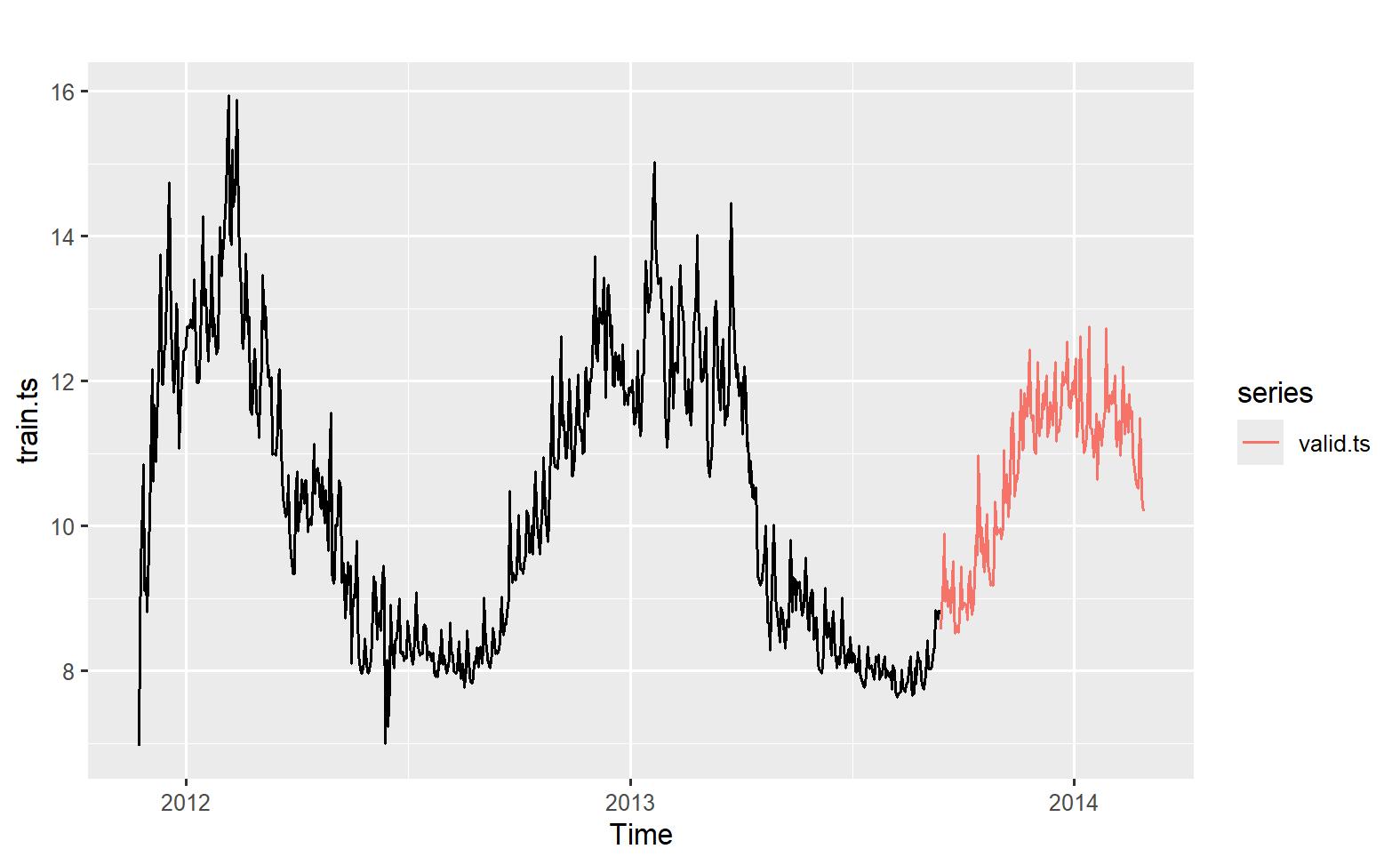
Initially, our team plotted the sum of the energy consumption for a given day but quickly realized that the study was rolling in nature. As households began to opt into the study, there were fewer houses at the start of the dataset This led us to take the average of each day’s consumption.
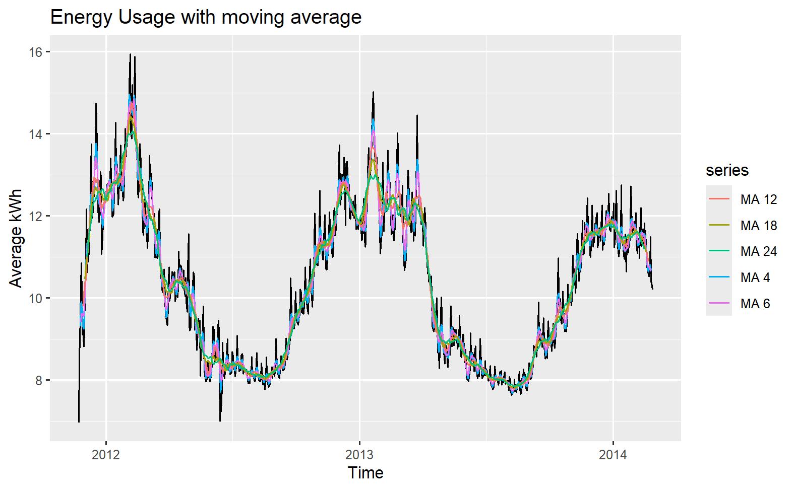
The plot showed seasonality in the data, with demand generally beginning to spike in September before peaking in January and starting to decline until July. Overall, however, there was a general negative trend, which may be due to the size of the sample rather than a strong indicator of the overall trajectory of London’s energy consumption
Forecasting Models
Linear Regression Model
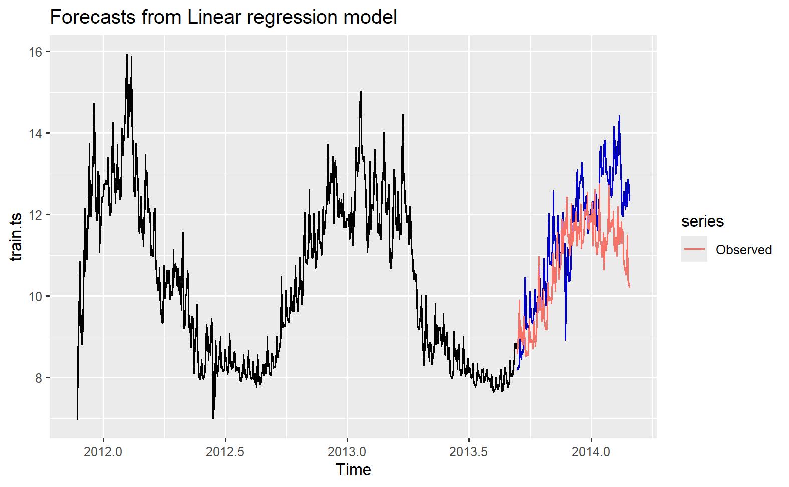
Our data was highly seasonal, so we wanted to ensure that we utilized its trend and seasonality when building our linear regression model. This model served as a baseline for our other models and was incorporated into the ensemble model. The forecast was reasonably accurate for a base model but generally overestimated energy consumption.
Holt Winters
One of the significant hurdles we encountered in our research was the seasonal nature of our data. While the Holt Winters model seemed like a natural fit due to its ability to integrate trend and seasonality into forecasts, it struggled with daily or weekly data To overcome this, we aggregated our daily averages into monthly averages and fit an ets model with additive error, additive trend, and additive seasonality This allowed us to smooth the data and factor in trend and seasonality. However, the primary downside was that it was not aggregated at the same level as the other data, preventing its use in an ensemble model.
Seasonal Naive
Naive methods are quick models that use previous values to build a simple model we can use as a baseline to compare future model performance. Our data was highly seasonal, so our team quickly found that a seasonal naive model performed more accurately. However, given that our data set does not follow a random walk, the optimal model is unlikely to be naive After conducting the forecasting of the remaining models, it is clear that the accuracy of the naive method is lower than that of the following models after incorporating seasonality. This finding
underscores the importance of considering seasonality in energy consumption forecasting models
Trailing moving average
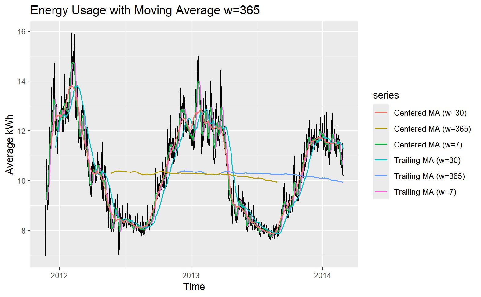
Our team used a lagged five-day moving average to predict the day's consumption. A smaller window failed to capture any short-term trends in the data, while a larger window was slow to react to changes and susceptible to being fooled by outliers For example, if a particular day had exceptionally high usage, the model would continue to predict higher-than-average temperatures for too long.
Seasonal Auto ARIMA
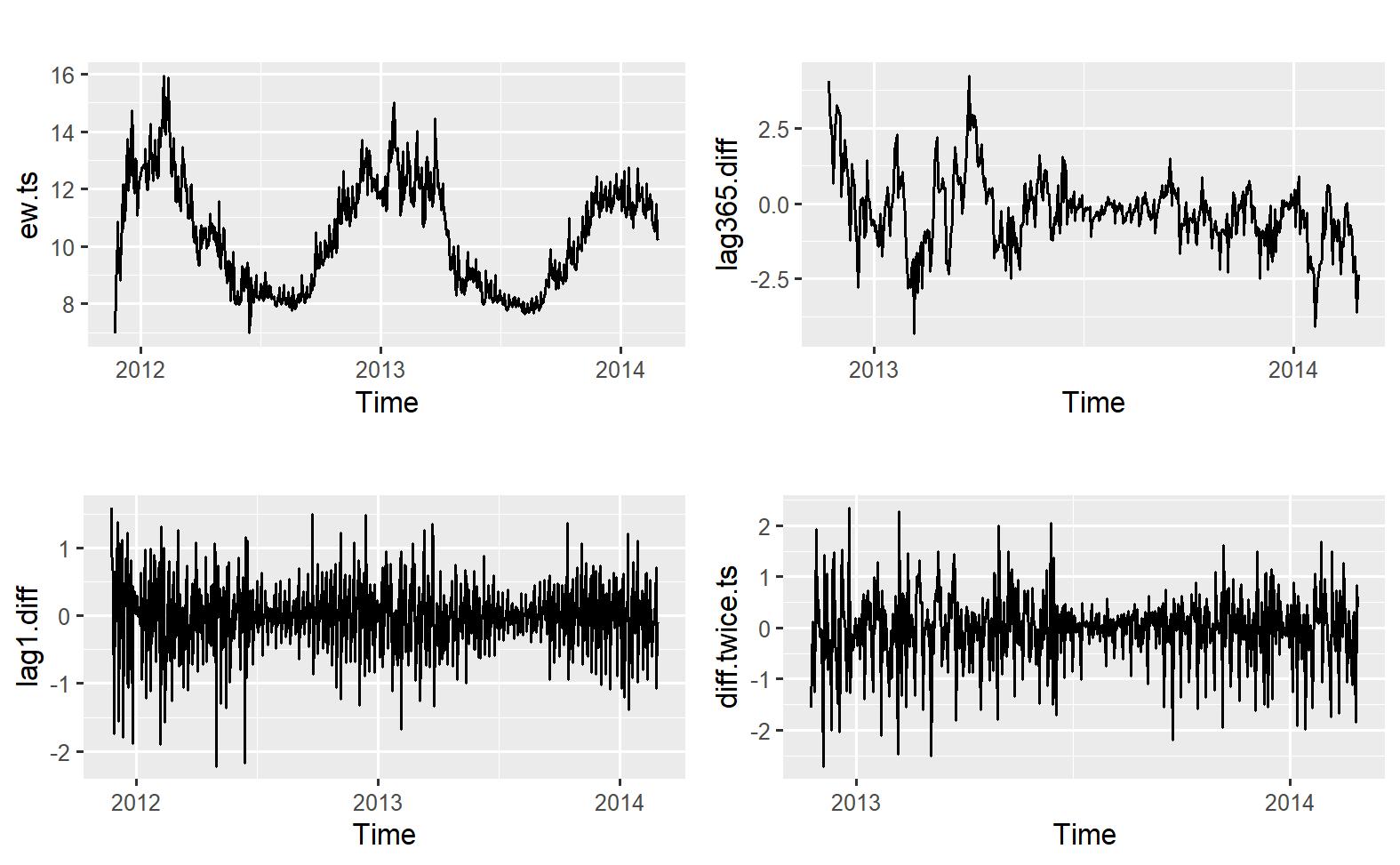
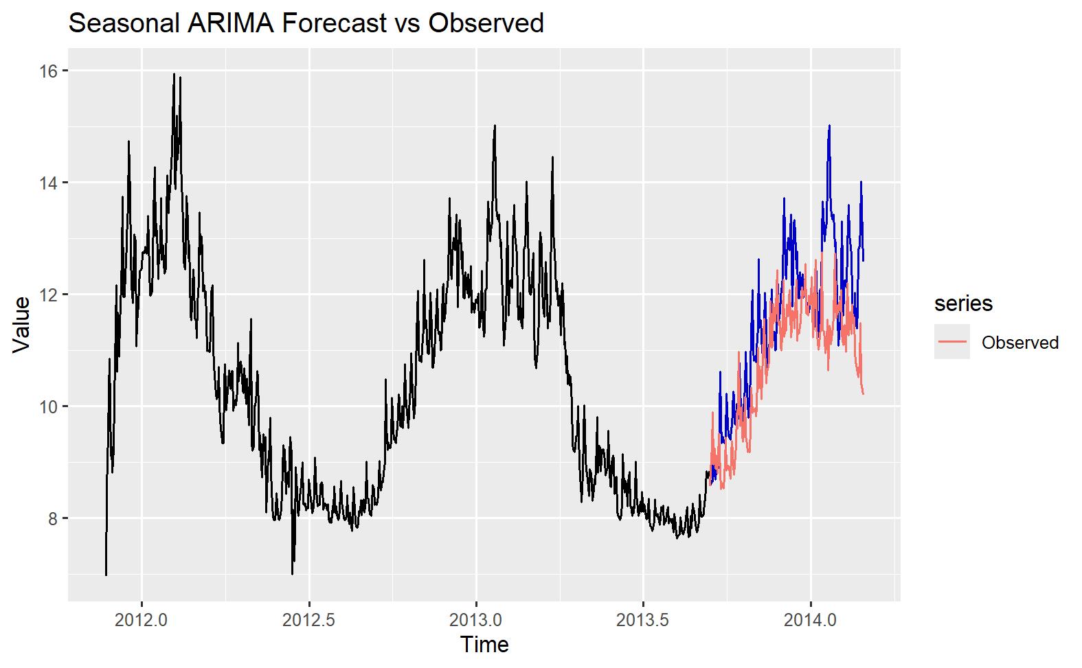
When developing an ARIMA model, we thought it would likely perform well because ARIMA models describe the autocorrelations in the data. We believed that being able to find relationships between neighboring values would be accurate due to seasonal energy demand. As with the other models, we opted for a seasonal ARIMA (SARIMA) model that utilizes autoregression, which uses past values (p lags) to predict future values. Next, it incorporates differencing to remove data trends and make it stationary It then includes moving averages to account for past forecast errors (q lags) to improve predictions. Lastly, it adds seasonal components to handle repeating patterns at fixed intervals.
ARIMAX
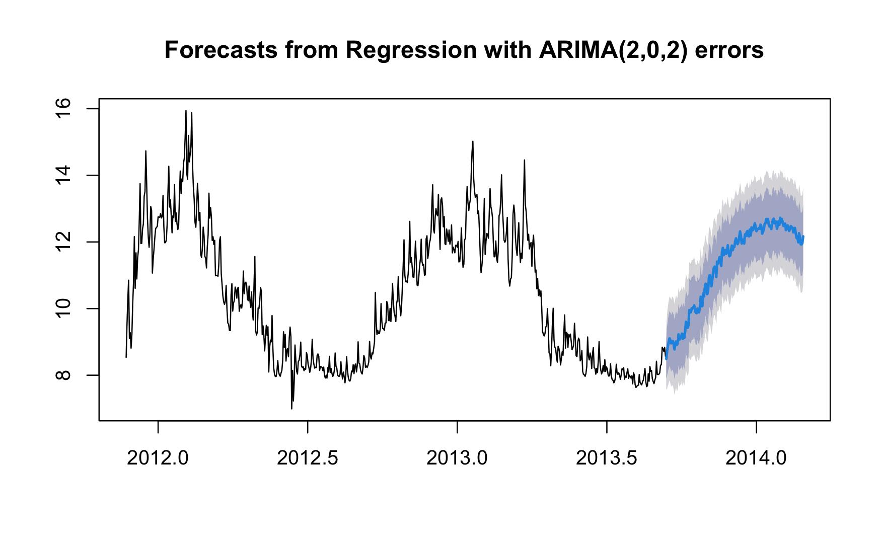
Our team also developed an ARIMAX model, which is an auto-ARIMA model that incorporates lag variables. The model included two autoregressive terms and a moving average component of two but did not include any differencing.
Advanced - Neural Net
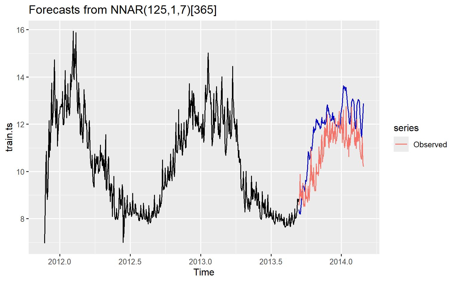
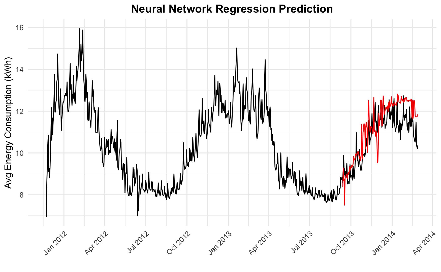
Our neural network was trained using a randomized grid search. We finally settled on 125 previous steps using only one seasonal value. The model also used seven hidden nodes to avoid overfitting It was trained over 20 epochs
Regression-Based Models - External Information
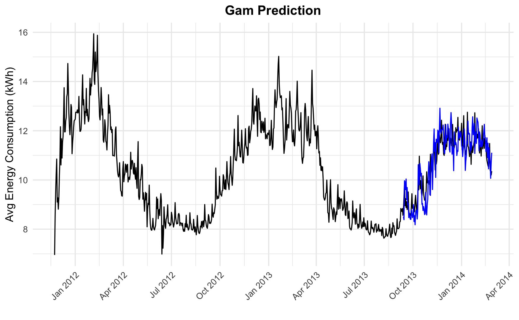
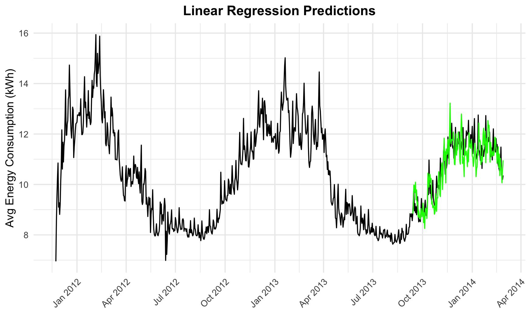
The team included lagged external weather information for our regression-based models, focusing on the previous day's mean temperature, cloud coverage, precipitation, snow, and sunshine. We opted to simplify the model and concentrated on the mean temperature, precipitation, and sunshine, as the snow and cloud cover were less statistically significant We settled on creating three models that utilized the lagged external information: a GAM model, a GLM model, and a neural network model The GAM, GLM, and neural network models were utilized in the regression-based ensemble model.
Forecast Accuracy
Conclusion
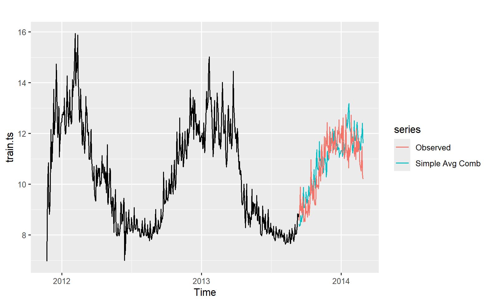
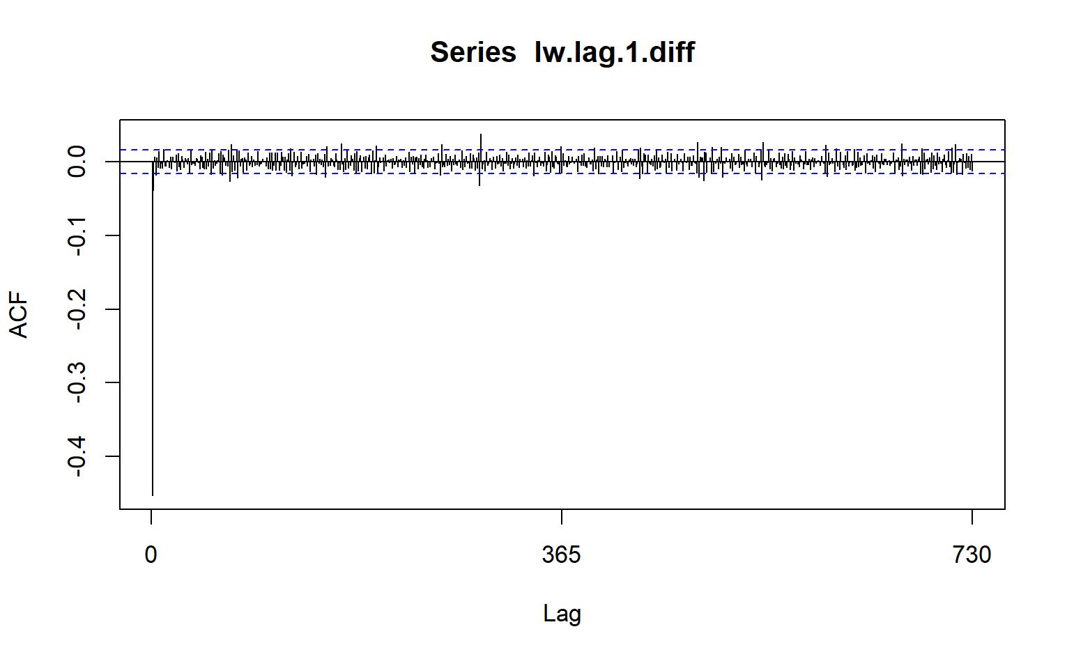
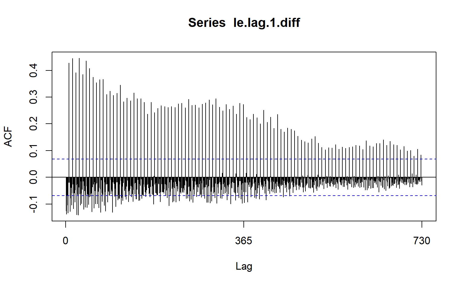
Our team found that neither the weather dataset nor the energy consumption datasets were random walks, allowing us to utilize both datasets to make predictions. Given the seasonality of the energy consumption of the dataset, the seasonal naive and seasonal ARIMA models performed well, capturing the overall seasonality of the data. The Holt-Winters model also performed adequately, though because of the daily nature of the data and the monthly nature of the Holt-Winters model, our team opted not to include it in our final ensemble model The final version of the time series regression ensemble model included the linear regression with seasonality and trend, seasonal ARIMA, the neural network, the seasonal naive, and the trailing average. While each model independently had varying accuracy, the ensemble model performed the best, with a MAPE of 2.664.
After creating an accurate ensemble model, our team tried incorporating lagged external predictors to see if variables like temperature, sunshine, and precipitation could help increase the overall accuracy of our model The lagged models generally outperformed the time series models individually, and the lagged ensemble model outperformed the ensemble regression model. Potential further analysis could include combining the best-performing lagged models with the top-performing time series models to create a more accurate model
In conclusion, our team feels it is possible to accurately predict energy consumption using time series forecasting and lagged variables This would enable NESO to predict energy consumption accurately and, in turn, protect the key stakeholders of London from energy shortages during peak demand.
References
Leake, J (2025, January 18) A Day in the Life of Blackout Britain: How Net Zero Electricity Rationing Would Play Out. Yahoo! News.
https://www.yahoo.com/news/day-life-blackout-britain-net-140000399.html
Owens, C (2020, October 16) Revisiting the Great Storm of 1987. The Blackout report
https://www.theblackoutreport.co.uk/2020/10/16/great-storm-1987/#:~:text=Biggest%20 Blackouts%20In%20History%3A%20The%20Great%20Storm%20Of%201987&text=Oc tober%201987%20saw%20the%20biggest,thousands%20of%20homes%20without%20p ower
Pathways to Net Zero Carbon by 2030. London City Hall. (2024, December 2).
https://www.london.gov.uk/programmes-strategies/environment-and-climate-change/clim ate-change/zero-carbon-london/pathways-net-zero-carbon-2030
Roller, S. (2021, September 21). When the Lights Went Out in Britain: The Story of the Three-Day Working Week. History Hit.
https://www historyhit com/when-the-lights-went-out-in-britain-the-story-of-the-three-da y-working-week/
Twomey, J. (2023, September 5). Remembering London’s Electrical Outage of 2003. South London News
https://londonnewsonline.co.uk/lifestyle/memories/remembering-londons-electrical-outag e-of-2003/#google vignette
Werr, E F (2022, May 16) London Weather Data Kaggle
https://www.kaggle.com/datasets/emmanuelfwerr/london-weather-data/data
Werr, E. F. (2022b, May 17). London Energy Data. Kaggle.
https://www kaggle com/datasets/emmanuelfwerr/london-homes-energy-data
Exhibit1:MergeddatasettrainingvalidationsplitofAveragekWhperday.
Exhibit2:LinearRegressionForecastWithSeasonalityandTrend
Exhibit3:DataVisualizationwithMovingAverages
Exhibit4:Movingaveragewithvariouswindowsizes
Exhibit6:TrendandSeasonalityRemovalUsingDi�erencing
Exhibit7:SeasonalArimaForecast
Exhibit8:NeuralNetForecastwithafewparameters
Exhibit9:SeasonalNaiveForecast
Exhibit10:CombinedSimpleAverageEnsembleModelForecast
Exhibit11:TrimmedMeanEnsembleModelForecast
Exhibit12:PlottingtheCombinedRegressionEnsemble
Exhibit16:ACFPlotofDi�erencedWeatherinLondon
Exhibit17:ACFPlotofDi�erencedEnergyConsumptioninLondon
Exhibit18:MovingAverageModel
Exhibit19:NeuralNetworkRegressionModel
Exhibit20:NeuralNetworkRegressionArchitecture
Exhibit21:GAMRegressionModel
Exhibit22:LinearRegressionPrediction
Exhibit23:LaggedEnsembleRegression
Exhibit24:ARIMAXModelForecast


