Chapter 9 • Beer, Farms, and Peas and the Use of Statistics
Historical Perspective
Sampling a Population
Understanding Descriptive Statistics
Using Descriptive Statistics
Using Histograms to Understand a Distribution
Normal Distributions
Chapter 10 • Sample in a Jar
Sampling in R
Repeating Our Sampling
Law of Large Numbers and the Central Limit
Theorem
Comparing Two Samples
Chapter 11 • Storage Wars
Importing Data Using RStudio
Accessing Excel Data
Accessing a Database
Comparing SQL and R for Accessing a Data Set
Accessing JSON Data
Chapter 12 • Pictures Versus Numbers
A Visualization Overview
Basic Plots in R
Using ggplot2
More Advanced ggplot2 Visualizations
Chapter 13 • Map Mashup
Creating Map Visualizations With ggplot2
Showing Points on a Map
A Map Visualization Example
Chapter 14 • Word Perfect
Reading in Text Files
Using the Text Mining Package
Creating Word Clouds
Chapter 15 • Happy Words?
Sentiment Analysis
Other Uses of Text Mining
Chapter 16 • Lining Up Our Models
What Is a Model?
Linear Modeling
An Example—Car Maintenance
Chapter 17 • Hi Ho, Hi Ho—Data Mining We Go
Data Mining Overview
Association Rules Data
Association Rules Mining
Exploring How the Association Rules Algorithm Works
Chapter 18 • What’s Your Vector, Victor?
Supervised and Unsupervised Learning
Supervised Learning via Support Vector Machines
Support Vector Machines in R
Chapter 19 • Shiny® Web Apps
Creating Web Applications in R
Deploying the Application
Chapter 20 • Big Data? Big Deal!
What Is Big Data?
The Tools for Big Data
Index
Preface
Welcome to IntroductiontoDataScience! This book began as the key ingredient to one of those massive open online courses, or MOOCs, and was written from the start to welcome people with a wide range of backgrounds into the world of data science. In the years following the MOOC we kept looking for, but never found, a better textbook to help our students learn the fundamentals of data science. Instead, over time, we kept refining and improving the book such that it has now become in integrated part of how we teach data science.
In that welcoming spirit, the book assumes no previous computer programming experience, nor does it require that students have a deep understanding of statistics. We have successfully used the book for both undergraduate and graduate level introductory courses. By using the free and open source R platform (R Core Team, 2016) as the basis for this book, we have also ensured that virtually everyone has access to the software needed to do data science. Even though it takes a while to get used to the R command line, our students have found that it opens up great opportunities to them, both academically and professionally.
In the pages that follow, we explain how to do data science by using R to read data sets, clean them up, visualize what’s happening, and perform different modeling techniques on the data. We explore both structured and unstructured data. The book explains, and we provide via an online repository, all the commands that teachers and learners need to do a wide range of data science tasks. If your goal is to consider the whole book in the span of 14 or 15 weeks, some of the earlier chapters can be grouped together or made optional for those learners with good working knowledge of data concepts. This approach allows an instructor to structure a semester so that each week of a
course can cover a different chapter and introduce a new data science concept.
Many thanks to Leah Fargotstein, Yvonne McDuffee, and the great team of folks at Sage Publications, who helped us turn our manuscript into a beautiful, professional product. We would also like to acknowledge our colleagues at the Syracuse University School of Information Studies, who have been very supportive in helping us get student feedback to improve this book. Go iSchool!
There were a number of reviewers we would like to thank who provided extremely valuable feedback during the development of the manuscript:
Luis F. Alvarez Leon, University of Southern California
Youngseek Kim, University of Kentucky
Nir Kshetri, UNC Greensboro
Richard N. Landers, Old Dominion University
John W. Mohr, University of California, Santa Barbara
Ryan T. Moore, American University and The Lab @ DC
Fred Oswald, Rice University
Eliot Rich, University at Albany, State University of New York
Ansaf Salleb-Aouissi, Columbia University
Toshiyuki Yuasa, University of Houston
About the Authors
Jeffrey S. Saltz, PhD (New Jersey Institute of Technology, 2006), is currently associate professor at Syracuse University, in the School of Information Studies. His research and teaching focus on helping organizations leverage information technology and data for competitive advantage. Specifically, Saltz’s current research focuses on the sociotechnical aspects of data science projects, such as how to coordinate and manage data science teams. In order to stay connected to the real world, Saltz consults with clients ranging from professional football teams to Fortune 500 organizations. Prior to becoming a professor, Saltz’s more than 20 years of industry experience focused on leveraging emerging technologies and data analytics to deliver innovative business solutions. In his last corporate role, at JPMorgan Chase, he reported to the firm’s chief information officer and drove technology innovation across the organization. Saltz also held several other key technology management positions at the company, including chief technology officer and chief information
architect. Saltz has also served as chief technology officer and principal investor at Goldman Sachs, where he invested and helped incubate technology start-ups. He started his career as a programmer, a project leader, and a consulting engineer with Digital Equipment Corp.
Jeffrey M. Stanton, PhD (University of Connecticut, 1997), is associate provost of academic affairs and professor of information studies at Syracuse University. Stanton’s research focuses on organizational behavior and technology. He is the author of InformationNation:EducatingtheNext GenerationofInformationProfessionals(2010), with Indira Guzman and Kathryn Stam. Stanton has also published many scholarly articles in peer-reviewed behavioral science journals, such as the Journalof AppliedPsychology,PersonnelPsychology,and Human Performance.His articles also appear in Journalof ComputationalScienceEducation,Computersand Security,CommunicationsoftheACM,Computersin HumanBehavior,the InternationalJournalofHumanComputerInteraction,InformationTechnologyand People,the JournalofInformationSystemsEducation, the JournalofDigitalInformation,Surveillanceand
Society,and Behaviour&InformationTechnology . He also has published numerous book chapters on data science, privacy, research methods, and program evaluation. Stanton’s methodological expertise is in psychometrics, with published works on the measurement of job satisfaction and job stress. Dr. Stanton’s research has been supported through 18 grants and supplements, including the National Science Foundation’s CAREER award.
For some, the term datascienceevokes images of statisticians in white lab coats staring fixedly at blinking computer screens filled with scrolling numbers. Nothing could be farther from the truth. First, statisticians do not wear lab coats: this fashion statement is reserved for biologists, physicians, and others who have to keep their clothes clean in environments filled with unusual fluids. Second, much of the data in the world is non-numeric and unstructured. In this context, unstructured means that the data are not arranged in neat rows and columns. Think of a web page full of photographs and short messages among friends: very few numbers to work with there. While it is certainly true that companies, schools, and governments use plenty of numeric information—sales of products, grade point averages, and tax assessments are a few examples— there is lots of other information in the world that mathematicians and statisticians look at and cringe. So, while it is always useful to have great math skills, there is much to be accomplished in the world of data science for those of us who are presently more comfortable working with words, lists, photographs, sounds, and other kinds of information.
In addition, data science is much more than simply analyzing data. There are many people who enjoy analyzing data and who could happily spend all day looking at histograms and averages, but for those who prefer other activities, data science offers a range of roles and requires a range of skills. Let’s consider this idea by thinking about some of the data involved in buying a box of cereal. Whatever your cereal preferences—fruity, chocolaty, fibrous, or nutty—you prepare for the purchase by writing “cereal” on your grocery list. Already your planned purchase is a piece of data, also called a datum, albeit a pencil scribble on the back on an envelope that only you can read. When you get to the grocery store, you use your datum as a reminder to grab that jumbo box of
FruityChocoBoms off the shelf and put it in your cart. At the checkout line, the cashier scans the barcode on your box, and the cash register logs the price. Back in the warehouse, a computer tells the stock manager that it is time to request another order from the distributor, because your purchase was one of the last boxes in the store. You also have a coupon for your big box, and the cashier scans that, giving you a predetermined discount. At the end of the week, a report of all the scanned manufacturer coupons gets uploaded to the cereal company so they can issue a reimbursement to the grocery store for all of the coupon discounts they have handed out to customers. Finally, at the end of the month a store manager looks at a colorful collection of pie charts showing all the different kinds of cereal that were sold and, on the basis of strong sales of fruity cereals, decides to offer more varieties of these on the store’s limited shelf space next month. So the small piece of information that began as a scribble on your grocery list ended up in many different places, most notably on the desk of a manager as an aid to decision making. On the trip from your pencil to the manager’s desk, the datum went through many transformations. In addition to the computers where the datum might have stopped by or stayed on for the long term, lots of other pieces of hardware—such as the barcode scanner—were involved in collecting, manipulating, transmitting, and storing the datum. In addition, many different pieces of software were used to organize, aggregate, visualize, and present the datum. Finally, many different human systems were involved in working with the datum. People decided which systems to buy and install, who should get access to what kinds of data, and what would happen to the data after its immediate purpose was fulfilled. The personnel of the grocery chain and its partners made a thousand other detailed decisions and negotiations before the scenario described earlier could become reality.
The Steps in Doing Data Science
Obviously, data scientists are not involved in all of these steps. Data scientists don’t design and build computers or barcode readers, for instance. So where would the data scientists play the most valuable role? Generally speaking, data scientists play the most active roles in the four As of data: data architecture, data acquisition, data analysis, and data archiving. Using our cereal example, let’s look at these roles one by one. First, with respect to architecture, it was important in the design of the point-of-sale system (what retailers call their cash registers and related gear) to think through in advance how different people would make use of the data coming through the system. The system architect, for example, had a keen appreciation that both the stock manager and the store manager would need to use the data scanned at the registers, albeit for somewhat different purposes. A data scientist would help the system architect by providing input on how the data would need to be routed and organized to support the analysis, visualization, and presentation of the data to the appropriate people.
Next, acquisition focuses on how the data are collected, and, importantly, how the data are represented prior to analysis and presentation. For example, each barcode represents a number that, by itself, is not very descriptive of the product it represents. At what point after the barcode scanner does its job should the number be associated with a text description of the product or its price or its net weight or its packaging type? Different barcodes are used for the same product (e.g., for different sized boxes of cereal). When should we make note that purchase X and purchase Y are the same product, just in different packages? Representing, transforming, grouping, and linking the data are all tasks that need to occur before the
data can be profitably analyzed, and these are all tasks in which the data scientist is actively involved. The analysis phase is where data scientists are most heavily involved. In this context, we are using analysis to include summarization of the data, using portions of data (samples) to make inferences about the larger context, and visualization of the data by presenting it in tables, graphs, and even animations. Although there are many technical, mathematical, and statistical aspects to these activities, keep in mind that the ultimate audience for data analysis is always a person or people. These people are the data users, and fulfilling their needs is the primary job of a data scientist. This point highlights the need for excellent communication skills in data science. The most sophisticated statistical analysis ever developed will be useless unless the results can be effectively communicated to the data user.
Finally, the data scientist must become involved in the archiving of the data. Preservation of collected data in a form that makes it highly reusable—what you might think of as data curation—is a difficult challenge because it is so hard to anticipate all of the future uses of the data. For example, when the developers of Twitter were working on how to store tweets, they probably never anticipated that tweets would be used to pinpoint earthquakes and tsunamis, but they had enough foresight to realize that geocodes—data that show the geographical location from which a tweet was sent—could be a useful element to store with the data.
The Skills Needed to Do Data Science
All in all, our cereal box and grocery store example helps to highlight where data scientists get involved and the skills they need. Here are some of the skills that the example suggested:
Learning the application domain: The data scientist must quickly learn how the data will be used in a particular context.
Communicating with data users: A data scientist must possess strong skills for learning the needs and preferences of users. The ability to translate back and forth between the technical terms of computing and statistics and the vocabulary of the application domain is a critical skill.
Seeing the big picture of a complex system: After developing an understanding of the application domain, the data scientist must imagine how data will move around among all of the relevant systems and people. Knowing how data can be represented: Data scientists must have a clear understanding about how data can be stored and linked, as well as about metadata (data that describe how other data are arranged).
Data transformation and analysis: When data become available for the use of decision makers, data scientists must know how to transform, summarize, and make inferences from the data. As noted earlier, being able to communicate the results of analyses to users is also a critical skill here.
Visualization and presentation: Although numbers often have the edge in precision and detail, a good data display (e.g., a bar chart) can often be a more effective means of communicating results to data users.
Attention to quality: No matter how good a set of data might be, there is no such thing as perfect data. Data scientists must know the limitations of the data they work with, know how to quantify its accuracy, and be able to make suggestions for improving the quality of the data in the future.
Ethical reasoning: If data are important enough to collect, they are often important enough to affect people’s lives. Data scientists must understand
important ethical issues such as privacy, and must be able to communicate the limitations of data to try to prevent misuse of data or analytical results. The skills and capabilities noted earlier are just the tip of the iceberg, of course, but notice what a wide range is represented here. While a keen understanding of numbers and mathematics is important, particularly for data analysis, the data scientist also needs to have excellent communication skills, be a great systems thinker, have a good eye for visual displays, and be highly capable of thinking critically about how data will be used to make decisions and affect people’s lives. Of course, there are very few people who are good at all of these things, so some of the people interested in data will specialize in one area, while others will become experts in another area. This highlights the importance of teamwork, as well. In this IntroductiontoDataSciencebook, a series of data problems of increasing complexity is used to illustrate the skills and capabilities needed by data scientists. The open source data analysis program known as R and its graphical user interface companion RStudio are used to work with real data examples to illustrate both the challenges of data science and some of the techniques used to address those challenges. To the greatest extent possible, real data sets reflecting important contemporary issues are used as the basis of the discussions.
Note that the field of big data is a very closely related area of focus. In short, big data is data science that is focused on very large data sets. Of course, no one actually defines a “very large data set,” but for our purposes we define big data as trying to analyze data sets that are so large that one cannot use RStudio. As an example of a big data problem to be solved, Macy’s (an online and brick-andmortar retailer) adjusts its pricing in near real time for 73 million items, based on demand and inventory (http://searchcio.techtarget.com/opinion/Ten-big-data-case-
studies-in-a-nutshell). As one might guess, the amount of data and calculations required for this type of analysis is too large for one computer running RStudio. However, the techniques covered in this book are conceptually similar to how one would approach the Macy’s challenge and the final chapter in the book provides an overview of some big data concepts.
Of course, no one book can cover the wide range of activities and capabilities involved in a field as diverse and broad as data science. Throughout the book references to other guides and resources provide the interested reader with access to additional information. In the open source spirit of R and RStudio these are, wherever possible, webbased and free. In fact, one of guides that appears most frequently in these pages is Wikipedia, the free, online, user-sourced encyclopedia. Although some teachers and librarians have legitimate complaints and concerns about Wikipedia, and it is admittedly not perfect, it is a very useful learning resource. Because it is free, because it covers about 50 times more topics than a printed encyclopedia, and because it keeps up with fast-moving topics (such as data science) better than printed sources, Wikipedia is very useful for getting a quick introduction to a topic. You can’t become an expert on a topic by consulting only Wikipedia, but you can certainly become smarter by starting there. Another very useful resource is Khan Academy. Most people think of Khan Academy as a set of videos that explain math concepts to middle and high school students, but thousands of adults around the world use Khan Academy as a refresher course for a range of topics or as a quick introduction to a topic that they never studied before. All the lessons at Khan Academy are free, and if you log in with a Google or Facebook account you can do exercises and keep track of your progress.
While Wikipedia and Khan Academy are great resources, there are many other resources available to help one learn data science. So, at the end of each chapter of this book is a list of sources. These sources provide a great place to start if you want to learn more about any of the topics the chapter does not explain in detail. It is valuable to have access to the Internet while you are reading so that you can follow some of the many links this book provides. Also, as you move into the sections in the book where open source software such as the R data analysis system is used, you will sometimes need to have access to a desktop or laptop computer where you can run these programs.
One last thing: The book presents topics in an order that should work well for people with little or no experience in computer science or statistics. If you already have knowledge, training, or experience in one or both of these areas, you should feel free to skip over some of the introductory material and move right into the topics and chapters that interest you most.
Understand the most granular representation of data within a computer.
Describe what a data set is.
Explain some basic R functions to build a data set.
The inventor of the World Wide Web, Sir Tim Berners-Lee, is often quoted as having said, “Data is not information, information is not knowledge, knowledge is not understanding, understanding is not wisdom,” but this quote is actually from Clifford Stoll, a well-known cyber sleuth.
The quote suggests a kind of pyramid, where data are the raw materials that make up the foundation at the bottom of the pile, and information, knowledge, understanding, and
wisdom represent higher and higher levels of the pyramid. In one sense, the major goal of a data scientist is to help people to turn data into information and onward up the pyramid. Before getting started on this goal, though, it is important to have a solid sense of what data actually are. (Notice that this book uses “data” as a plural noun. In common usage, you might hear “data” as both singular and plural.) If you have studied computer science or mathematics, you might find the discussion in this chapter somewhat redundant, so feel free to skip it. Otherwise, read on for an introduction to the most basic ingredient to the data scientist’s efforts: data.
A substantial amount of what we know and say about data in the present day comes from work by a U.S. mathematician named Claude Shannon. Shannon worked before, during, and after World War II on a variety of mathematical and engineering problems related to data and information. Not to go crazy with quotes or anything, but Shannon is quoted as having said, “The fundamental problem of communication is that of reproducing at one point either exactly or approximately a message selected at another point”
(http://math.harvard.edu/~ctm/home/text/others/shannon/e ntropy/entropy.pdf, 1). This quote helpfully captures key ideas about data that are important in this book by focusing on the idea of data as a message that moves from a source to a recipient. Think about the simplest possible message that you could send to another person over the phone, via a text message, or even in person. Let’s say that a friend had asked you a question, for example, whether you wanted to come to her house for dinner the next day. You can answer yes or no. You can call the person on the phone and say yes or no. You might have a bad connection, though, and your friend might not be able to hear you. Likewise, you could send her a text message with your answer, yes or no, and hope that she has her phone turned on so she can receive
the message. Or you could tell your friend face-to-face and hope that she does not have her earbuds turned up so loud that she couldn’t hear you. In all three cases, you have a one-bit message that you want to send to your friend, yes or no, with the goal of reducing her uncertainty about whether you will appear at her house for dinner the next day. Assuming that message gets through without being garbled or lost, you will have successfully transmitted one bit of information from you to her. Claude Shannon developed some mathematics, now often referred to as Information Theory, that carefully quantified how bits of data transmitted accurately from a source to a recipient can reduce uncertainty by providing information. A great deal of the computer networking equipment and software in the world today—and especially the huge linked worldwide network we call the Internet—is primarily concerned with this one basic task of getting bits of information from a source to a destination.
Storing Data—Using Bits and Bytes
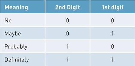
Once we are comfortable with the idea of a bit as the most basic unit of information, either “yes” or “no,” we can combine bits to make more-complicated structures. First, let’s switch labels just slightly. Instead of “no” we will start using zero, and instead of “yes” we will start using one. So we now have a single digit, albeit one that has only two possible states: zero or one (we’re temporarily making a rule against allowing any of the bigger digits like three or seven). This is in fact the origin of the word bit, which is a squashed down version of the phrase Binary digIT. A single binary digit can be zero (0) or one (1), but there is nothing stopping us from using more than one binary digit in our messages. Have a look at the example in the table below:
Here we have started to use two binary digits—two bits—to create a code book for four different messages that we might want to transmit to our friend about her dinner party. If we were certain that we would not attend, we would send her the message 0 0. If we definitely planned to attend, we would send her 1 1. But we have two additional possibilities, “maybe,” which is represented by 0 1, and “probably,” which is represented by 1 0. It is interesting to compare our original yes/no message of one bit with this new four-option message with two bits. In fact, every time you add a new bit you double the number of possible messages you can send. So three bits would give 8 options and four bits would give 16 options. How many options would there be for five bits?
When we get up to eight bits—which provides 256 different combinations—we finally have something of a reasonably useful size to work with. Eight bits is commonly referred to as a “byte”—this term probably started out as a play on words with the word bit. (Try looking up the wordnybble online!) A byte offers enough different combinations to encode all of the letters of the alphabet, including capital and small letters. There is an old rulebook called ASCII— the American Standard Code for Information Interchange— which matches up patterns of eight bits with the letters of the alphabet, punctuation, and a few other odds and ends. For example, the bit pattern 0100 0001 represents the
capital letter A and the next higher pattern, 0100 0010, represents capital B. Try looking up an ASCII table online (e.g., http://www.asciitable.com/) and you can find all of the combinations. Note that the codes might not actually be shown in binary because it is so difficult for people to read long strings of ones and zeroes. Instead, you might see the equivalent codes shown in hexadecimal (base 16), octal (base 8), or the most familiar form that we all use every day, base 10. Although you might remember base conversions from high school math class, it would be a good idea to practice this—particularly the conversions between binary, hexadecimal, and decimal (base 10). You might also enjoy Vi Hart’sBinaryHandDancevideo at Khan Academy (search for this at http://www.khanacademy.org or follow the link at the end of the chapter). Most of the work we do in this book will be in decimal, but more-complex work with data often requires understanding hexadecimal and being able to know how a hexadecimal number, like 0xA3, translates into a bit pattern. Try searching online for “binary conversion tutorial” and you will find lots of useful sites.
Combining Bytes into Larger Structures
Now that we have the idea of a byte as a small collection of bits (usually eight) that can be used to store and transmit things like letters and punctuation marks, we can start to build up to bigger and better things. First, it is very easy to see that we can put bytes together into lists in order to make a string of letters, often referred to as a character string or text string. If we have a piece of text, like “this is a piece of text,” we can use a collection of bytes to represent it like this:
Now nobody wants to look at that, let alone encode or decode it by hand, but fortunately, the computers and software we use these days takes care of the conversion and storage automatically. For example, we can tell the open source data language R to store “this is a piece of text” for us like this:
> myText <- “this is a piece of text” We can be certain that inside the computer there is a long list of zeroes and ones that represent the text that we just stored. By the way, in order to be able to get our piece of text back later on, we have made a kind of storage label for it (the word “myText” above). Anytime that we want to remember our piece of text or use it for something else, we can use the label myText to open up the chunk of computer memory where we have put that long list of binary digits that represent our text. The left-pointing arrow made up out of the less-than character (<) and the dash character (–) gives R the command to take what is on the right-hand side (the quoted text) and put it into what is on the lefthand side (the storage area we have labeled myText). Some people call this the assignment arrow, and it is used in some computer languages to make it clear to the human who writes or reads it which direction the information is flowing. Yay! We just explored our first line of R code. But don’t worry about actually writing code just yet: We will discuss installing R and writing R code in Chapter 3. From the computer’s standpoint, it is even simpler to store, remember, and manipulate numbers instead of text. Remember that an eight-bit byte can hold 256 combinations, so just using that very small amount we could store the numbers from 0 to 255. (Of course, we could have also done 1 to 256, but much of the counting and numbering that goes on in computers starts with zero instead of one.) Really, though, 255 is not much to work
with. We couldn’t count the number of houses in most towns or the number of cars in a large parking garage unless we can count higher than 255. If we put together two bytes to make 16 bits we can count from zero up to 65,535, but that is still not enough for some of the really big numbers in the world today (e.g., there are more than 200 million cars in the United States alone). Most of the time, if we want to be flexible in representing an integer (a number with no decimals), we use four bytes stuck together. Four bytes stuck together is a total of 32 bits, and that allows us to store an integer as high as 4,294,967,295. Things get slightly more complicated when we want to store a negative number or a number that has digits after the decimal point. If you are curious, try looking up “two’s complement” for more information about how signed numbers are stored and “floating point” for information about how numbers with digits after the decimal point are stored. For our purposes in this book, the most important thing to remember is that text is stored differently than numbers, and among numbers integers are stored differently than floating point. Later we will find that it is sometimes necessary to convert between these different representations, so it is always important to know how it is represented. So far, we have mainly looked at how to store one thing at a time, like one number or one letter, but when we are solving problems with data we often need to store a group of related things together. The simplest place to start is with a list of things that are all stored in the same way. For example, we could have a list of integers, where each thing in the list is the age of a person in your family. The list might look like this: 43, 42, 12, 8, 5. The first two numbers are the ages of the parents and the last three numbers are the ages of the kids. Naturally, inside the computer each number is stored in binary, but fortunately we don’t have to type them in that way or look at them that way. Because
there are no decimal points, these are just plain integers and a 32-bit integer (4 bytes) is more than enough to store each one. This list contains items that are all the same type or mode.
Creating a Data Set in R
The open source data program R refers to a list where all of the items are of the same mode as a vector. We can create a vector with R very easily by listing the numbers, separated by commas and inside parentheses:
> c(43, 42, 12, 8, 5)
The letter c in front of the opening parenthesis stands for combine, which means to join things together. Slightly obscure, but easy enough to get used to with some practice. We can also put in some of what we learned earlier to store our vector in a named location (remember that a vector is list of items of the same mode/type):
> myFamilyAges <- c(43, 42, 12, 8, 5)
We have just created our first data set. It is very small, for sure, only five items, but it is also very useful for illustrating several major concepts about data. Here’s a recap:
In the heart of the computer, all data are represented in binary. One binary digit, or bit, is the smallest chunk of data that we can send from one place to another. Although all data are at heart binary, computers and software help to represent data in more convenient forms for people to see. Three important representations are “character” for representing text, “integer” for representing numbers with no digits after the decimal point, and “floating point” for numbers that might have digits after the decimal point. The numbers in our tiny data set just above are integers. Numbers and text can be collected into lists, which the open source program R calls vectors. A vector has a length, which is the number of items in it, and a mode
which is the type of data stored in the vector. The vector we were just working on has a length of five and a mode of integer.
In order to be able to remember where we stored a piece of data, most computer programs, including R, give us a way of labeling a chunk of computer memory. We chose to give the five-item vector up above the name myFamilyAges. Some people might refer to this named list as a variable because the value of it varies, depending on which member of the list you are examining.
If we gather together one or more variables into a sensible group, we can refer to them together as a data set. Usually, it doesn’t make sense to refer to something with just one variable as a data set, so usually we need at least two variables. Technically, though, even our very simple myFamilyAges counts as a data set, albeit a very tiny one.
Later in the book we will install and run the open source R data program and learn more about how to create data sets, summarize the information in those data sets, and perform some simple calculations and transformations on those data sets.
Chapter Challenge
Discover the meaning of Boolean Logic and the rules for and,or,not,and exclusiveor. Once you have studied this for a while, write down on a piece of paper, without looking, all the binary operations that demonstrate these rules.