Issuu

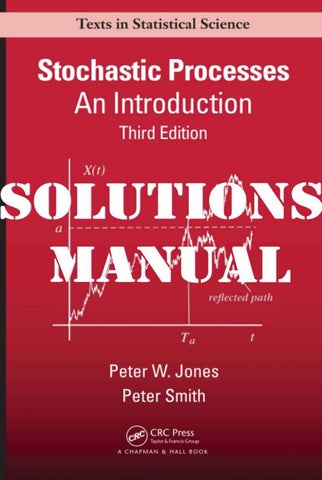
Stochastic Processes: An Introduction Solutions Manual Third Edition c Peter W Jones and Peter Smith School of Computing and Mathematics, Keele University, UK

Preface The website includes answers and solutions of all the end-of-chapter problems in the textbook Stochastic Processes: An Introduction, third edition. We hope that they will prove helpful to lecturers in designing courses, and to students as a source of model examples. The original problems as numbered in the text are also included. There are obviously references to results and examples from the textbook, and the manual should be viewed as a supplement to the book. To help identify the sections and chapters, the full contents of Stochastic Processes follow this preface. Every effort has been made to eliminate misprints or errors (or worse), and the authors, who were responsible for the LaTeX code, apologise in advance for any which occur. Peter W. Jones Peter Smith

Keele, 2017

Contents of Stochastic Processes Chapter 1: Some Background in Probability 1.1 Introduction 1.2 Probability 1.3 Conditional probability and independence 1.4 Discrete random variables 1.5 Continuous random variables 1.6 Mean and variance 1.7 Some standard discrete probability distributions 1.8 Some standard continuous probability distributions 1.9 Generating functions 1.10 Conditional expectation Problems Chapter 2: Some Gambling Problems 2.1 Gambler’s ruin 2.2 Probability of ruin 2.3 Some numerical simulations 2.4 Expected duration of the game 2.5 Some variations of gambler’s ruin 2.5.1 The infinitely rich opponent 2.5.2 The generous gambler 2.5.3 Changing the stakes Problems Chapter 3: Random Walks 3.1 Introduction 3.2 Unrestricted random walks 3.3 Probability distribution after n steps 3.4 First returns of the symmetric random walk Problems Chapter 4: Markov Chains 4.1 States and transitions 4.2 Transition probabilities 4.3 General two-state Markov chain 4.4 Powers of the transition matrix for the m-state chain 4.5 Gambler’s ruin as a Markov chain 4.6 Classification of states 4.7 Classification of chains 4.8 A wildlife Markov chain model Problems Chapter 5: Poisson Processes 5.1 Introduction 5.2 The Poisson process 5.3 Partition theorem approach 5.4 Iterative method 5.5 The generating function 5.6 Variance for the Poisson process

5.7 Arrival times 5.8 Summary of the Poisson process Problems Chapter 6: Birth and Death Processes 6.1 Introduction 6.2 The birth process 6.3 Birth process: generating function equation 6.4 The death process 6.5 The combined birth and death process 6.6 General population processes Problems Chapter 7: Queues 7.1 Introduction 7.2 The single server queue 7.3 The stationary process 7.4 Queues with multiple servers 7.5 Queues with fixed service times 7.6 Classification of queues Problems Chapter 8: Reliability and Renewal 8.1 Introduction 8.2 The reliability function 8.3 The exponential distribution and reliability 8.4 Mean time to failure 8.5 Reliability of series and parallel systems 8.6 Renewal processes 8.7 Expected number of renewals Problems Chapter 9: Branching and Other Random Processes 9.1 Introduction 9.2 Generational growth 9.3 Mean and variance 9.4 Probability of extinction 9.5 Branching processes and martingales 9.6 Stopping rules 9.7 A continuous time epidemic 9.8 A discrete time epidemic model 9.9 Deterministic epidemic models 9.10 An iterative scheme for the simple epidemic Problems Chapter 10: Brownian Motion: Wiener Process 10.1 Introduction 10.2 Brownian motion 10.3 Wiener process as a limit of a random walk 10.4 Brownian motion with drift 10.5 Scaling 10.6 First visit times 3

10.7 Other Brownian motions in one dimension 10.8 Brownian motion in more than one dimension Problems Chapter 11: Computer Simulations and Projects

Contents of the Solutions Manual Chapter 1: Some Background in Probability Chapter 2: Some Gambling Problems Chapter 3: Random Walks

Chapter 4: Markov Chains

Chapter 5: Poisson Processes

Chapter 6: Birth and Death Processes Chapter 7: Queues

105

Chapter 8: Reliability and Renewal

121

Chapter 9: Branching and Other Random Processes Chapter 10: Brownian Motion: Wiener Process

150

130

Chapter 1

Some background in probability 1.1. The Venn diagram of three events is shown in Figure 1.5(in the text). Indicate on the diagram the following events: (a) A ∪ B; (b) A ∪ (B ∪ C); (c) A ∩ (B ∪ C); (d) (A ∩ C)c ; (e) (A ∩ B) ∪ C c . S

S A

(a)

(b) S

S A

(c)

(d) S B

C (e)

Figure 1.1: The events are shaded in Figure 1.1. 1.2. In a random experiment, A, B, C are three events. In set notation write down expressions for the events: (a) only A occurs; (b) all three events A, B, C occur; (c) A and B occur but C does not; (d) at least one of the events A, B, C occurs; (e) exactly one of the events A, B, C occurs; (f ) not more than two of the events occur. (a) A ∩ (B ∪ C)c ; (b) A ∩ (B ∩ C) = A ∩ B ∩ C; (c) (A ∩ B) ∩ C c ; (d) A ∪ B ∪ C;

(e) A ∩ (B ∪ C)c represents an event in A but not in either B nor C: therefore the answer is (A ∩ (B ∪ C)c ) ∪ (B ∩ (A ∪ C)c ) ∪ (C ∩ (A ∪ B)c ). (f) A ∩ B ∩ C 1.3. For two events A and B, P(A) = 0.4, P(B) = 0.5 and P(A ∩ B) = 0.3. Calculate (a) P(A ∪ B); (b) P(A ∩ B c ); (c) P(Ac ∪ B c ). (a) From (1.1) P(A ∪ B) = P(A) + P(B) − P(A ∩ B), it follows that P(A ∪ B) = 0.4 + 0.5 − 0.3 = 0.6. (b) Since A = (A ∩ B c ) ∪ (A ∩ B) and A ∩ B c , and A ∩ B are mutually exclusive, then, P(A) = P[(A ∩ B c ) ∪ (A ∩ B)] = P(A ∩ B c ) + P(A ∩ B), so that

P(A ∩ B c ) = P(A) − P(A ∩ B) = 0.4 − 0.3 = 0.1.

P(Ac ∪ B c ) = P[(A ∩ B)c ] = 1 − P(A ∩ B) = 1 − 0.3 = 0.7. 1.4. Two distinguishable fair dice a and b are rolled. What are the elements of the sample space? What is the probability that the sum of the face values of the two dice is 9? What is the probability that at least one 5 or at least one 3 appears? The 36 elements of the sample space are listed in Example 1.1. The event A1 , that the sum is 9, is given by A1 = {(3, 6), (4, 5), (5, 4), (6, 3)}.

4 Hence P = 36 = 19 . Let A2 be the event that at least one 5 or at least one 3 appears. Then by counting the elements in 20 the sample space in Example 1.1, P(A2 ) = 36 = 59 .

1.5. Two distinguishable fair dice a and b are rolled. What is the probability that the sum of the faces is not more than 6? Let the random variable X be the sum of the faces. By counting events in the sample space in Example 15 5 1.1, P(X) = 36 = 12 . 1.6. For the probability generating function 1

G(s) = (2 − s)− 2 find {pn } and its mean.

Note that G(1) = 1. Using the binomial theorem (see the Appendix) ∞

1 1 1 1 X − 21 G(s) = √ (1 − s)− 2 = √ 2 2 2 n=0 n

Hence 1 p0 = √ , 2

1 1 pn = √ n 22

The mean is

n s 2

− 21 , n

− 21 0

(n = 1, 2, . . .).

µ = G′ (1) = 21 (2 − s)− 2

where

s=1

= 12 .

= 1.

1.7. Find the probability generating function G(s) of the Poisson distribution (see Section 1.7) with parameter α given by e−α αn pn = , n = 0, 1, 2, . . . . n! Determine the mean and variance of {pn } from the generating function. Given pn = e−α αn /n!, the generating function is given by G(s) =

∞ X

p n sn =

n=0

∞ X e−α αn sn

n=0

= e−α

∞ X (αs)n

n=0

= eα(s−1) .

The mean and variance are given by µ = G′ (1) =

d α(s−1) = α, e s=1 ds

σ 2 = G′′ (1) + G′ (1) − [G′ (1)]2 = [α2 eα(s−1) + αeα(s−1) − α2 e2α(s−1) ]s=1 = α. 1.8. A panel contains n warning lights. The times to failure of the lights are the independent random variables T1 , T2 , . . . , Tn which have exponential distributions with parameters α1 , α2 , . . . , αn respectively. Let T be the random variable of the time to first failure, that is T = min{T1 , T2 , . . . , Tn }.

Show that T has an exponential distribution with parameter

j=1

αj .

The probability that no warning light has failed by time t is P(T ≥ t)

P(T1 ≥ t ∩ T2 ≥ t ∩ · · · ∩ Tn ≥ t)

P(T1 ≥ t)P(T2 ≥ t) · · · P(Tn ≥ t)

e−α1 t e−α2 t · · · e−αn t = e−(α1 +α2 +···+αn )t .

1.9. The geometric distribution with parameter p is given by p(x) = q x−1 p,

x = 1, 2, . . .

where q = 1−p (see Section 1.7). Find its probability generating function. Calculate the mean and variance of the geometric distribution from its pgf. The generating function is given by G(s) =

∞ X x−1

∞

pX ps p qs = , (qs)x = q q 1 − qs 1 − qs

psx =

x=1

using the formula for the sum of a geometric series. The mean is given by ps 1 − qs

d G (s) = ds

d µ = G (1) = ds ′

For the variance, ′′

is required. Hence

= s=1

pqs p + 1 − qs (1 − qs)2

p (1 − qs)2

σ 2 = G′′ (1) + G′ (1) − [G′ (1)]2 =

= s=1

2pq . (1 − qs)3

1 1 q 2q + − 2 = 2. p2 p p p

1 . p

1.10. Two distinguishable fair dice a and b are rolled. What are the probabilities that: (a) at least one 4 appears; (b) only one 4 appears; (c) the sum of the face values is 6; (d) the sum of the face values is 5 and one 3 is shown; (e) the sum of the face values is 5 or only one 3 is shown? From the Table in Example 1.1: (a) If A1 is the event that at least one 4 appears, then P(A1 ) = 11 . 36 10 5 (b) If A2 is the event that only one 4 appears, then P(A2 ) = 36 = 18 . 5 (c) If A3 is the event that the sum of the faces is 6, then P(A3 ) = 36 . 2 1 (d) If A4 is the event that the face values is 5 and one 3 is shown, then P(A4 ) = 36 = 18 . 5 10 = 18 . (e) If A5 is the event that the sum of the faces is 5 or only one 3 is shown, then P(A5 ) = 36 1.11. Two distinguishable fair dice a and b are rolled. What is the expected sum of the face values? What is the variance of the sum of the face values? Let N be the random variable representing the sum x + y, where x and y are face values of the two dice. Then " 6 # 6 6 6 X X 1 XX 1 E(N ) = (x + y) = 6 x+6 y = 7. 36 36 x=1 y=1

x=1

y=1

and

V(N )

1 XX (x + y)2 − 72 E(N ) − E(N ) = 36 2

x=1 y=1

= =

X 2 1 12 x +2 36 x=1

6 X x=1

!2 #

− 49

35 329 − 49 = = 5.833 . . . . 6 6

1.12. Three distinguishable fair dice a, b and c are rolled. How many possible outcomes are there for the faces shown? When the dice are rolled, what is the probability that just two dice show the same face values and the third one is different? The sample space contains 63 = 216 elements of the form, (in the order a, b, c), S = {(i, j, k)},

(i = 1, . . . , 6; j = 1, . . . , 6; k = 1, . . . , 6).

Let A be the required event. Suppose that a and b have the same face values, which can occur in 6 ways, and that c has a different face value which can occurs in 5 ways. Hence the total number of ways in which a and b are the same but c is different is 6 × 5 = 30 ways. The faces b and c, and c and a could also be the same so that the total number of ways for the possible outcome is 3 × 30 = 90 ways. Therefore the required probability is 90 5 P(A) = = . 216 12 1.13. In a sample space S, the events B and C are mutually exclusive, but A and B, are not. Show that P(A ∪ (B ∪ C)) = P(A) + P(B) + P(C) − P(A ∩ (B ∪ C)). From a well-shuffled pack of 52 playing cards a single card is randomly drawn. Find the probability that it is a club or an ace or the king of hearts. From (1.1) (in the book) P(A ∪ (B ∪ C)) = P(A) + P(B ∪ C) − P(A ∩ (B ∪ C))

(i).

Since B and C are mutually exclusive, P(B ∪ C) = P(B) + P(C).

(ii)

From (i) and (ii), it follows that P(A ∪ (B ∪ C)) = P(A) + P(B) + P(C) − P(A ∩ (B ∪ C)). Let A be the event that the card is a club, B the event that it is an ace, and C the event that it is the king of hearts. We require P(A ∩ (B ∪ C)). Since B and C are mutually exclusive, we can use the result above. The individual probabilities are P(A) =

1 13 = ; 52 4

4 1 = ; 52 13

P(B) =

P(C) =

1 , 52

and since A ∩ (B ∪ C) = A ∩ B (A and C are mutually exclusive) is the ace of clubs, P(A ∩ (B ∪ C)) = Finally

1 1 1 17 1 + + − = . 4 13 52 52 52

P(A ∪ (B ∪ C)) = 1.14. Show that f (x) =

  0

x<0 0≤x≤a x>a

1 2a 1 −(x−a)/a e 2a



1 . 52

is a possible probability density function. Find the corresponding probability function. Check the density function as follows:

Z ∞

f (x)dx

1 2a

−∞

Z a

dx +

The probability function is given by, for 0 ≤ x ≤ a, F (x) =

Z ∞

e−(x−a)/a dx

1 − 21 [e−(x−a)/a ]∞ a = 1. 2

Z x

1 2a

f (u)du =

−∞

Z x 0

x 1 du = , 2a 2a

and, for x > a, by F (x)

Z x

f (u)du =

Z a 0

1 du + 2a

1 1 − [ae−(u−a)/a ]xa 2 2a 1 1 − e−(x−a)/a . 2

= =

Z a 0

1 −(u−a)/a e du 2a

1.15. A biased coin is tossed. The probability of a head is p. The coin is tossed until the first head appears. Let the random variable N be the total number of tosses including the first head. Find P(N = n), and its pgf G(s). Find the expected value of the number of tosses. The probability that the total number of throws is n (including the head) until the first head appears is (assuming independent events) (n−1) times

{

P(N = n) = (1 − p)(1 − p) · · · (1 − p) p = (1 − p)n−1 p,

(n ≥ 1)

The probability generating function is given by G(s)

∞ X

n=1

(1 − p)n−1 psn =

∞

p X [(1 − p)s]n 1−p n=1

s(1 − p) ps p · = , 1 − p [1 − s(1 − p)] 1 − s(1 − p)

after summing the geometric series. For the mean, we require G′ (s) given by, G′ (s) =

sp(1 − p) p p + = . [1 − s(1 − p)] [1 − s(1 − p)]2 [1 − s(1 − p)]2

The mean is given by µ = G′ (1) = 1/p. 1.16. The m random variables X1 , X2 , . . . , Xm are independent and identically distributed each with a gamma distribution with parameters n and α. The random variable Y is defined by Y = X1 + X2 + · · · + Xm . Using the moment generating function, find the mean and variance of Y . The probability density function for the gamma distribution with parameters n and α is f (x) =

αn n−1 −αx x e . Γ(n)

It was shown in Section 1.9 that the moment generating function for Y is given, in general, by MY (s) = [MX (s)]m . For any gamma distribution X with parameters α and n, its mgf is MX =

α n

Hence MY (s)

E(Y ) =

nm s −nm α = 1− α−s α nm(nm + 1) 2 nm 1+ s+ s + ··· α 2α2

= =

Hence

α−s

nm , α

V(Y ) = E(Y 2 ) − [E(Y )]2 =

nm . α2

1.17. A probability generating function with parameter 0 < α < 1 is given by G(s) =

1 − α(1 − s) . 1 + α(1 − s)

Find pn = P(N = n) by expanding the series in powers of s. What is the mean of the probability function {pn }? Applying the binomial theorem G(s)

= =

1 − α(1 − s) (1 − α)[1 + (α/(1 − α))s] = 1 + α(1 − s) (1 + α)[1 − (α/(1 + α))s]

1−α 1+α

∞

∞ X αs n αs 1−α 1+α

1−α X α 1+α 1+α n=0

n=0

sn +

∞

α X α 1+α 1+α n=0

sn+1 .

The summation of the two series leads to G(s)

∞

1−α X α 1+α 1+α

n=0

∞

n=1

1−α , 1+α

p0 =

s +

∞ n X α n

pn =

1+α

n=1

1−α 2 X α + 1+α 1+α 1+α

= Hence

2αn , (1 + α)n+1

(n = 1, 2, . . .).

The mean is given by d G (1) = ds ′

1 − α(1 − s) 1 + α(1 − s)

s=1

2α [1 + a(1 − s)]2

= 2α s=1

1.18. Find the moment generating function of the random variables X which has the uniform distribution

f (x) =

1/(b − a) 0

a≤x≤b for all other values of x

Deduce E(X n ). The moment generating function of the uniform distribution is MX (s)

Z b

1 1 bs exs dx = [e − eas ] b−a b−as ∞

n=1

Hence E(X) =

1 (b + a), 2

1 X bn − a n b−a n!

sn−1

bn+1 − an+1 , (n + 1)(b − a)

E(X n ) =

(n = 2, 3, . . .).

1.19. A random variable X has the normal distribution with mean µ and variance σ 2 . Find its moment generating function. By definition MX (s)

E(eXs ) =

1 √ σ 2π

Z ∞

exp

−∞

Z ∞

−∞

(x − µ)2 dx 2σ 2

2σ 2 xs − (x − µ)2 dx 2σ 2

Apply the substitution x = µ + σ(v − σs): then MX (s)

esx exp −

Z ∞

1 2 1 √ e− 2 v dv 2π −∞

exp(sµ + 21 σ 2 s2 )

exp(sµ + 12 σ 2 s2 ) × 1 = exp(sµ + 21 σ 2 s2 )

(see the Appendix for the integral). Expansion of the exponential function in powers of s gives MX (s) = 1 + µs +

1 2 (µ + σ 2 )s2 + · · · . 2

So, for example, E(X 2 ) = µ2 + σ 2 .

1.20. Find the probability generating functions of the following distributions, in which 0 < p < 1: (a) Bernoulli distribution: pn = pn (1 − p)1−n , (n = 0, 1); (b) geometric distribution: pn = p(1 − p)n−1 , (n = 1, 2, . . .); (c) negative binomial distribution with parameter r expressed in the form: pn =

r+n−1 r p (1 − p)n , r−1

(n = 0, 1, 2, . . .)

where r is a positive integer. In each case find also the mean and variance of the distribution using the probability generating function. (a) For the Bernoulli distribution G(s) = p0 + p1 s = (1 − p) + ps. The mean is given by

µ = G′ (1) = p,

and the variance by

σ 2 = G′′ (1) + G′ (1) − [G′ (1)]2 = p − p2 = p(1 − p).

(b) For the geometric distribution (with q = 1 − p) G(s) =

∞ X

pq n−1 sn = ps

n=1

∞ X

(qs)n =

n=0

ps 1 − qs

summing the geometric series. The mean and variance are given by ′

µ = G (1) =

p (1 − qs)2

σ 2 = G′′ (1) + G′ (1) − [G′ (1)]2 =

= s=1

2pq (1 − qs)3

∞ X r+n−1 r n n n=0

r−1

p q s =p

pr (1 − qs)r

1 , p +

s=1

1 1 1−p − 2 = . p p p2

r(r + 1) (qs)2 + · · · 1 + r(qs) + 2!

The derivatives of G(s) are given by G′ (s) =

rqpr , (1 − qs)r+1

G′′ (s) =

r(r + 1)q 2 pr . (1 − qs)r+2

Hence the mean and variance are given by µ = G′ (1) = σ 2 = G′′ (1) + G′ (1) − [G′ (1)]2 =

rq , p

r(r + 1)q 2 rq r2 q2 rq + − 2 = 2 2 p p p p

1.21. A word of five letters is transmitted by code to a receiver. The transmission signal is weak, and there is a 5% probability that any letter is in error independently of the others. What is the probability that the word is received correctly? The same result is transmitted a second time with the same errors in the signal. If the same word is received, what is the probability now that the word is correct?

Let A1 , A2 , A3 , A4 , A5 be the events that the letters in the word are correct. Since the events are independent, the probability that the word is correctly transmitted is P(A1 ∩ A2 ∩ A3 ∩ A4 ∩ A5 ) = P(A1 )P(A2 )P(A3 )P(A4 )P(A5 ) = 0.955 ≈ 0.774. If a letter is sent a second time the probability that one error occurs twice is 0.052 = 0.0025. Hence the probability that the letter is correct is 0.9975. For 5 letters the probability that the word is correct is 0.99755 ≈ 0.988. 1.22. A binary code of 500 bits is transmitted across a weak link. The probability that any bit has a transmission error is 0.0004 independently of the others. (a) What is the probability that only the first bit fails? (b) What is the probability that the code is transmitted successfully? (c) What is the probability that at least two bits fail? (a) Probability = 0.0004 × 0.9996499 = 0.000328... (b) Probability = 0.1638... (c) Probability is 500 X j=2

0.0004j × 0.9996500−j = 0.01750.

For any practical purposes the upper limit in the series can be replaced by 7 for sufficient accuracy. 1.23. The source of a beam of light is a perpendicular distance d from a wall of length 2a, with the perpendicular from the source meeting the wall at its midpoint. The source emits a pulse of light randomly in a direction θ, the angle between the direction of the pulse and the perpendicular is chosen uniformly in the range − tan−1 (a/d) ≤ θ ≤ tan−1 (a/d). Find the probability distribution of x (−a ≤ x ≤ a) where the pulses hit the wall. Show that its density function is given by f (x) =

d , 2(x2 + d2 ) tan−1 (a/d)

(this the density function of a Cauchy distribution). If a → ∞, what can you say about the mean of this distribution? Figure 1.2 shows the beam and wall. Let X be the random variable representing any displacement

wall

-a

beam 0

Figure 1.2: Source and beam for Problem 1.23 between −a and x. Then P(−a ≤ X ≤ x)

= = =

P(−a ≤ d tan θ ≤ x)

P(tan−1 (−a/d) + tan−1 (x/d)) tan−1 (x/d) + tan−1 (a/d) 2 tan−1 (a/d)

by uniformity. The density is given by f (x)

The mean is given by µ=

tan−1 (x/d) + tan−1 (a/d) 2 tan−1 (a/d)

d dx

d 2(x2 + d2 ) tan−1 (a/d)

Z a

xd dx = 0, 2 + d2 ) tan−1 (a/d) 2(x −a

since the integrand is an odd function and the limits are ±a. For the infinite wall the integral defining the mean becomes divergent. 1.24. Suppose that the random variable X can take the integer values 0, 1, 2, . . .. Let pj and qj be the probabilities pj = P(X = j), qj = P(X > j), (j = 0, 1, 2, . . .). Show that, if G(s) =

∞ X

p j sj ,

H(s) =

j=0

then (1 − s)H(s) = 1 − G(s). Show also that E(X) = H(1).

∞ X

qj sj ,

j=0

Using the series for H(s), (1 − s)H(s)

(1 − s) q0 +

∞ X j=0

q0 −

∞ X j=0

∞ X j=1

qj sj =

qj sj −

∞ X

qj sj+1

j=0

(qj − qj−1 )sj

∞ X

P(X = j)sj

j=1

1 − p0 −

∞ X j=1

pj sj = 1 − G(s)

Note that generally H(s) is not a probability generating function. The mean of the random variable X is given by E(X) =

∞ X

jpj = G′ (1) = H(1),

j=1

differentiating the formula above. 1.25 In a lottery players can choose q numbers from the consecutive integers 1, 2, . . . , n (q < n). The player wins if r numbers (3 ≤ r ≤ q) from q agree with those numbers of the q numbers randomly chosen from the n integers. Show that the probability of r numbers being correct is

q r

n−q q−r

n . q

Compute the probabilities if n = 49, q = 6, r = 3, 4, 5, 6 (the UK lottery). This is a combinatorial problem. There are

n q

possible combinations of choosing q numbers from n. From the n − q numbers which are not randomly chosen this must include the q − r losing numbers: they can be chosen in

n−q q−r

ways. Also there are

q r

ways of choosing the r numbers from q. Hence the probability of winning in the lottery is

n−q q−r

q r

n . q

If n = 49, q = 6, and r = 3, 4, 5, 6, then the probabilities are given in the table: r 3 4 5 6

formula

43 6

43 6 49 2

43 6 49 5

43 6 49 6

exact probability

approximation

8815 499422

0.0177

645 665896

0.000969

43 2330636

0.0000184

43 6

0.0000000715

The chance of correctly choosing 6 numbers is 1 in 13,983,816. 1.26. A count of the second edition of this book showed that it contains 181,142 Roman letters (not case sensitive: Greek not included). The table of the frequency of the letters. Frequency table a b c d e f g h i

13011 4687 6499 5943 15273 5441 3751 9868 12827

j k l m n o p q r

561 1424 6916 5487 14265 11082 6891 1103 10756

s t u v w x y z

12327 15074 5708 2742 3370 2361 3212 563

The most frequent letter is e closely followed by t, n and a. However, since this a mathematical textbook there is considerable distortion compared with a piece of prose caused by the extensive use of symbols particularly in equations. What is the probability that a letter is i ? What is the probability that a letter is a vowel a, e, i , o, u? A word count shows that the word probability occurs 821 times. From the table P(i) = 12827/181142 = 0.0708... P(vowel) = (13011 + 15273 + 12827 + 11082 + 5708)/181142 = 0.3196.... 1.27 Using the table of probabilities in Example 1.9, calculate the conditional probabilities and random variable of the conditional expectation E(Y |X). From Example 1.9 the table of mass functions is

p(xi , yj ) x1 x2 x3

y1 0.25 0.05 0.05

y2 0 0.10 0.25

y3 0.05 0.15 0.10

The required conditional probabilities are: pY (y1 |x1 ) = p(x1 , y1 )/

3 X

p(x1 , yj ) = 0.25/0.3 =

j=1

pY (y2 |x1 ) = p(x1 , y2 )/ pY (y3 |x1 ) = p(x1 , y3 )/

3 X

5 , 6

p(x1 , yj ) = 0,

j=1

p(x1 , yj ) = 0.5/0.3 =

j=1

1 1 pY (y1 |x2 ) = , pY (y2 |x2 ) = , 6 3 5 1 pY (y2 |x3 ) = , pY (y1 |x3 ) = , 8 8 It follows that the conditional probabilities are:

1 , 6

1 , 2 1 pY (y3 |x5 ) = . 4 pY (y3 |x2 ) =

E(Y |X = x1 ) =

3 X

yi p(yj |x1 ) = 1 ×

5 1 4 +2×0+3× = , 6 6 3

E(Y |X = x2 ) =

3 X

yj p(yj |x2 ) = 1 ×

1 1 7 1 +2× +3× = , 6 3 2 3

E(Y |X = x3 ) =

j=1

3 X j=1

p(yj |x3 ) = 1 ×

1 5 1 17 +2× +3× = . 8 8 4 8

}, and Hence the random variable U = E(Y |X)) takes the values { 34 , 73 , 17 8 E(U ) = E[E(Y |X)] =

7 17 39 4 × 0.3 + × 0.3 + × 0.4 = . 3 3 8 20

For comparison E(Y ) = 1 × 0.35 + 2 × 0.35 + 3 × 0.3 =

39 20

which agrees with E(U ). 1.28. (a) Show that the moment generating function (mgf ) of a N (µ, σ 2 ) random variable is exp(µs + 1 2 2 σ s ). 2 (b) Use (a) to identify the distribution of Z = (X − µ)/σ where X is N (µ, σ 2 ).

(d) A sequence Xi (i = 1, 2, . . . n) of n independent normally distributed random variables has mean µi Pn X . If Zi are n iid standard normal random variables, and variance σ 2i . Derive the distribution of i i=1 Pn what is the distribution of Z . i i=1

(e) Consider the sequence of random variables in (c): find the distribution of a Xi , where the i=1 i P n ai ’s (i = 1, 2, . . . , n) are constants. What is the distribution of the mean of the Xi ’s, namely Xi /n? i−1 (a) The mgf of N (µ, σ 2 ) is (if X is the random variable) MX (s) = E(esX ) = √

1 2πσ

Z ∞

−∞

exp(sx) exp −

(x − µ)2 dx. 2σ 2

Using the substitution y = (x − µ)/σ, MX (s)

Z ∞

y2 dy exp[(yσ + µ)s] exp − 2 −∞

1 √ 2π

1 1 √ exp[µs + s2 σ 2 ] 2 2π

exp[µs + 21 s2 σ 2 ],

Z ∞

1 exp[− (y − sσ 2 )2 ]dy 2 −∞

(see Appendix for the value of the integral) (b) As in (a) use the substitution z = (x − µ)/σ so that the mgf MZ (s) = E(esZ ) = √

1 2πσ

Z ∞

exp(zs) exp −

−∞

(z − µ)2 dz = exp( 21 σ 2 ), 2σ 2

which is the mgf of a standardised normal distribution N (0, 1). (c) For the random variable Y = aX + b, the mgf is MY (s) = E(eaX+b ) = eb E(eaX ). From (a) it can be deduced that Y has the normal distribution N (aµ + b, a2 σ 2 ). (d) As in Section 1.9 the mgf of W = MW (s)

i=1

Xi is

E[exp(

n X

Xi )] =

i=1

exp s

. Hence W is normal N

" n X

n X

µi ,

MXi (s)

i=1

µi + 12 s2

i=1

n Y

n X

σ 2i

i=1

σ2 i=1 i

The distribution of the iid standard normal random variables Zi is therefore, from above N (0, n). (e) Let U =

i=1

ai Xi . Then the mgf of U is given by MU (s) = E[exp(

n X

ai Xi )] =

n Y

Mai Xi (s)

i=1

From (c) ai Xi has the normal distribution N [ai µi , a2i σ 2 ]. Hence U has the normal distribution N

" n X

ai µi ,

i=1

The distribution of the mean

i=1

n X 2

ai σ 2 .

i=1

Xi /n is therefore normal given by N

" n X i=1

µi /n,

n X i=1

σ /n

1.29. (a) Let Z have a standard normal distribution, show that the mgf of Z 2 is (1 − 2s)− 2 . This is the mgf of a χ2 distribution on 1 degree of freedom (χ21 ). Hence Z 2 has a χ21 distribution.

(b) Let Z1 , Z2 . . . , Zn be a sequence of n iid standard normal random variables . Show that the mgf of Y =

n X

Zi2

i=1

is (1 − 2s)− 2 n , which is the mgf of a χ2n distribution. (c) Find the mean and variance of Y in (b).

(a) If U = Z 2 , then the mgf of Z 2 is given by MU (s)

= =

1 E[exp(sZ )] = √ 2 π 2

1 √ 2 π

Z ∞

−∞

Z ∞

exp(sz 2 ) exp(− 21 z 2 )dz

−∞ 1

exp[( 12 − s)z 2 ]dz = (1 − 2s)− 2

(see Appendix for value of the integral). (b) Result 1

follows from Problem 28(d).

MY (s) = (1 − 2s)− 2 n

MY′ (s) = n(1 − 2s)− 2 n−1 , so that Therefore

MY′ (0) = n, E(Z 2 ) = MY′ (0) = n,

MY′′ (s) = n(n + 2)(1 − 2s)− 2 n−2 , MY′′ (0) = n(n + 2). σ 2 = MY′′ (0) − [MY′ (0)]2 = 2n.

Chapter 2

Some gambling problems 2.1. In the standard gambler’s ruin problem with total stake a and gambler’s stake k and the gambler’s probability of winning at each play is p, calculate the probability of ruin in the following cases; (a) a = 100, k = 5, p = 0.6; (b) a = 80, k = 70, p = 0.45; (c) a = 50, k = 40, p = 0.5. Also find the expected duration in each case. For p 6= 12 , the probability of ruin uk and the expected duration of the game dk are given by uk =

sk − sa , 1 − sa

(a) uk ≈ 0.132, dk ≈ 409. (b) uk ≈ 0.866, dk ≈ 592. (c) For p = 21 , uk =

dk =

1 a(1 − sk ) k− . 1 − 2p (1 − sa )

a−k , a

dk = k(a − k).

so that uk = 0.2, dk = 400. 2.2. In a casino game based on the standard gambler’s ruin, the gambler and the dealer each start with 20 tokens and one token is bet on at each play. The game continues until one player has no further tokens. It is decreed that the probability that any gambler is ruined is 0.52 to protect the casino’s profit. What should the probability that the gambler wins at each play be? The probability of ruin is sk − sa , 1 − sa where k = 20, a = 40, p is the probability that the gambler wins at each play, and s = (1 − p)/p. Let r = s20 . Then u = r/(1 + r), so that r = u/(1 − u) and u=

s= Finally, with u = 0.52, p=

u 1/20 1−u

(1 − u)1/20 1 = ≈ 0.498999. 1+s (1 − u)1/20 + u1/20

2.3. Find general solutions of the following difference equations: (a) uk+1 − 4uk + 3uk−1 = 0; (b) 7uk+2 − 8uk+1 + uk = 0; (c) uk+1 − 3uk + uk−1 + uk−2 = 0.

(d) puk+2 − uk + (1 − p)uk−1 = 0, (a) The characteristic equation is

(0 < p < 1).

m2 − 4m + 3 = 0

which has the solutions m1 = 1 and m2 = 3. The general solution is uk = Amk1 + Bmk2 = A + 3k B, where A and B are any constants. (b) The characteristic equation is

7m2 − 8m + 1 = 0,

which has the solutions m1 = 1 and m2 = 71 . The general solution is uk = A +

1 B. 7k

(c) The characteristic equation is the cubic equation m3 − 3m2 + m + 1 = (m − 1)(m2 − 2m − 1) = 0, √ √ which has the solutions m1 = 1, m2 = 1 + 2, and m3 = 1 − 2. The general solution is √ √ uk = A + B(1 + 2)k + C(1 − 2)k . (d) The characteristic equation is the cubic equation pm3 − m + (1 − p) = (m − 1)(pm2 + pm − (1 − p)) = 0, √ √ which has the solutions m1 = 1, m2 = − 21 + 12 [(4 − 3p)/p] and m3 = − 21 − 21 [(4 − 3p)/p]. The general solution is uk = A + Bmk2 + Cmk3 . 2.4 Solve the following difference equations subject to the given boundary conditions: (a) uk+1 − 6uk + 5uk−1 = 0, u0 = 1, u4 = 0; (b) uk+1 − 2uk + uk−1 = 0, u0 = 1, u20 = 0; (c) dk+1 − 2dk + dk−1 = −2, d0 = 0, d10 = 0; (d) uk+2 − 3uk + 2uk−1 = 0, u0 = 1, u10 = 0, 3u9 = 2u8 . (a) The charactedristic equation is

m2 − 6m + 5 = 0,

which has the solutions m1 = 1 and m2 = 5. Therefore the general solution is given by uk = A + 5k B. The boundary conditions u0 = 1, u4 = 0 imply A + 54 B = 0,

A + B = 1,

which have the solutions A = 625/624 and B = −1/624. The required solution is uk =

625 5k − . 624 624

(b) The characteristic equation is m2 − 2m + 1 = (m − 1)2 = 0, which has the repeated solution m = 1. Using the rule for repeated roots, uk = A + Bk.