Solutions
Manual for Thomas' Calculus
15th Edition by Hass, Heil, Weir
ISBN: 9780137615582
ISBN: 9780137615582
SUNY Empire State College
Based on the original work by George B. Thomas, Jr
Massachusetts Institute of Technology
as revised by
Joel Hass
University of California, Davis
Christopher Heil
Georgia Institute of Technology
Maurice D. Weir
Naval Postgraduate School

The author and publisher of this book have used their best efforts in preparing this book. These efforts include the development, research, and testing of the theories and programs to determine their effectiveness. The author and publisher make no warranty of any kind, expressed or implied, with regard to these programs or the documentation contained in this book. The author and publisher shall not be liable in any event for incidental or consequential damages in connection with, or arising out of, the furnishing, performance, or use of these programs.
Reproduced by Pearson from electronic files supplied by the author.
Copyright © 2023, 2018, 2014 by Pearson Education, Inc. or its affiliates, 221 River Street, Hoboken, NJ 07030. All Rights Reserved. Manufactured in the United States of America. This publication is protected by copyright, and permission should be obtained from the publisher prior to any prohibited reproduction, storage in a retrieval system, or transmission in any form or by any means, electronic, mechanical, photocopying, recording, or otherwise. For information regarding permissions, request forms, and the appropriate contacts within the Pearson Education Global Rights and Permissions department, please visit www.pearsoned.com/permissions/.
PEARSON and REVEL are exclusive trademarks owned by Pearson Education, Inc. or its affiliates in the U.S. and/or other countries.
Unless otherwise indicated herein, any third-party trademarks, logos, or icons that may appear in this work are the property of their respective owners, and any references to third-party trademarks, logos, icons, or other trade dress are for demonstrative or descriptive purposes only. Such references are not intended to imply any sponsorship, endorsement, authorization, or promotion of Pearson’s products by the owners of such marks, or any relationship between the owner and Pearson Education, Inc., or its affiliates, authors, licensees, or distributors.
ISBN-13: 978-0-13-761600-8
ISBN-10: 0-13-761600-7
1.1 Functions and Their Graphs 1
1.2 Combining Functions; Shifting and Scaling Graphs 9
1.3 Trigonometric Functions 19
1.4 Graphing with Software 27
Practice Exercises 32
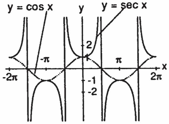
Additional and Advanced Exercises 40
2.1 Rates of Change and Tangents to Curves 43
2.2 Limit of a Function and Limit Laws 47
2.3 The Precise Definition of a Limit 57
2.4 One-Sided Limits 65
2.5 Continuity 70
2.6 Limits Involving Infinity; Asymptotes of Graphs 75
Practice Exercises 86
Additional and Advanced Exercises 92
3.1 Tangents and the Derivative at a Point 99
3.2 The Derivative as a Function 105
3.3 Differentiation Rules 116
3.4 The Derivative as a Rate of Change 121
3.5 Derivatives of Trigonometric Functions 127
3.6 The Chain Rule 134
3.7 Implicit Differentiation 146
3.8 Related Rates 155
3.9 Linearization and Differentials 160
Practice Exercises 167
Additional and Advanced Exercises 180
4.1 Extreme Values of Functions on Closed Intervals 187
4.2 The Mean Value Theorem 195
4.3 Monotonic Functions and the First Derivative Test 201
4.4 Concavity and Curve Sketching 213
4.5 Applied Optimization 236
4.6 Newton's Method 251
4.7 Antiderivatives 255
Practice Exercises 263
Additional and Advanced Exercises 277
5.1 Area and Estimating with Finite Sums 285
5.2 Sigma Notation and Limits of Finite Sums 290
5.3 The Definite Integral 296
5.4 The Fundamental Theorem of Calculus 312
5.5 Indefinite Integrals and the Substitution Method 322
5.6 Definite Integral Substitutions and the Area Between Curves 328 Practice Exercises 345
Additional and Advanced Exercises 355
6.1 Volumes Using Cross-Sections 361
6.2 Volumes Using Cylindrical Shells 373
6.3 Arc Length 384
6.4 Areas of Surfaces of Revolution 391
6.5 Work and Fluid Forces 397
6.6 Moments and Centers of Mass 408
Practice Exercises 422
Additional and Advanced Exercises 432
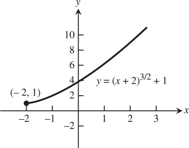
7.1 Inverse Functions and Their Derivatives 439
7.2 Natural Logarithms 449
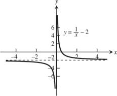
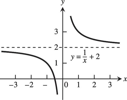
7.3 Exponential Functions 457
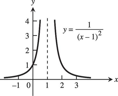
7.4 Exponential Change and Separable Differential Equations 472
7.5 Indeterminate Forms and L’Hôpital’s Rule 478
7.6 Inverse Trigonometric Functions 487
7.7 Hyperbolic Functions 501
7.8 Relative Rates of Growth 510
Practice Exercises 515
Additional and Advanced Exercises 529
8.1 Using Basic Integration Formulas 533
8.2 Integration by Parts 544
8.3 Trigonometric Integrals 558
8.4 Trigonometric Substitutions 567
8.5 Integration of Rational Functions by Partial Fractions 577
8.6 Integral Tables and Computer Algebra Systems 588
8.7 Numerical Integration 599
8.8 Improper Integrals 612
8.9 Probability 626
Practice Exercises 634
Additional and Advanced Exercises 648
9.1 Solutions, Slope Fields, and Euler's Method 657
9.2 First-Order Linear Equations 667
9.3 Applications 671
9.4 Graphical Solutions of Autonomous Equations 675
9.5 Systems of Equations and Phase Planes 683
Practice Exercises 688
Additional and Advanced Exercises 696
10.1 Sequences 699
10.2 Infinite Series 711
10.3 The Integral Test 720
10.4 Comparison Tests 728
10.5 Absolute Convergence; The Ratio and Root Tests 738
10.6 Alternating Series and Conditional Convergence 745
10.7 Power Series 755
10.8 Taylor and Maclaurin Series 767
10.9 Convergence of Taylor Series 773
10.10 The Binomial Series and Applications of Taylor Series 781
Practice Exercises 791
Additional and Advanced Exercises 801
11.1 Parametrizations of Plane Curves 807
11.2 Calculus with Parametric Curves 816
11.3 Polar Coordinates 825
11.4 Graphing Polar Coordinate Equations 831
11.5 Areas and Lengths in Polar Coordinates 839
11.6 Conic Sections 845
11.7 Conics in Polar Coordinates 856
Practice Exercises 866
Additional and Advanced Exercises 877
12.1 Three-Dimensional Coordinate Systems 883
12.2 Vectors 888
12.3 The Dot Product 894
12.4 The Cross Product 900
12.5 Lines and Planes in Space 908
12.6 Cylinders and Quadric Surfaces 916
Practice Exercises 922
Additional and Advanced Exercises 930
13.1 Curves in Space and Their Tangents 937
13.2 Integrals of Vector Functions; Projectile Motion 944
13.3 Arc Length in Space 953
13.4 Curvature and Normal Vectors of a Curve 957
13.5 Tangential and Normal Components of Acceleration 965
13.6 Velocity and Acceleration in Polar Coordinates 972
Practice Exercises 974
Additional and Advanced Exercises 981
14.1 Functions of Several Variables 985
14.2 Limits and Continuity in Higher Dimensions 995
14.3 Partial Derivatives 1003
14.4 The Chain Rule 1012
14.5 Directional Derivatives and Gradient Vectors 1025
14.6 Tangent Planes and Differentials 1030
14.7 Extreme Values and Saddle Points 1038
14.8 Lagrange Multipliers 1055
14.9 Taylor's Formula for Two Variables 1066
14.10 Partial Derivatives with Constrained Variables 1070
Practice Exercises 1073
Additional and Advanced Exercises 1090
15.1 Double and Iterated Integrals over Rectangles 1097
15.2 Double Integrals over General Regions 1100
15.3 Area by Double Integration 1115
15.4 Double Integrals in Polar Form 1120
15.5 Triple Integrals in Rectangular Coordinates 1126
15.6 Moments and Centers of Mass 1132
15.7 Triple Integrals in Cylindrical and Spherical Coordinates 1139
15.8 Substitutions in Multiple Integrals 1152
Practice Exercises 1160
Additional and Advanced Exercises 1168
16.1 Line Integrals 1175
16.2 Vector Fields and Line Integrals: Work, Circulation, and Flux 1181
16.3 Path Independence, Conservative Fields, and Potential Functions 1193
16.4 Green's Theorem in the Plane 1199
16.5 Surfaces and Area 1207
16.6 Surface Integrals 1217
16.7 Stokes' Theorem 1228
16.8 The Divergence Theorem and a Unified Theory 1235 Practice Exercises 1242
Additional and Advanced Exercises 1252
17.1 Second-Order Linear Equations 1257
17.2 Nonhomogeneous Linear Equations 1263
17.3 Applications 1275
17.4 Euler Equations 1281
17.5 Power-Series Solutions 1284
18.1 Complex Numbers 1295
18.2 Functions of a Complex Variable 1297
18.3 Derivatives 1298
18.4 The Cauchy-Riemann Equations 1299
18.5 Complex Power Series 1299
18.6 Some Complex Functions 1300
18.7 Conformal Maps 1302
Additional and Advanced Exercises 1303
19.1 Periodic Functions 1305
19.2 Summing Sines and Cosines 1305
19.3 Vectors and Approximation in Three and More Dimensions 1307
19.4 Approximation of Functions 1310
19.5 Advanced Topic: The Haar System and Wavelets 1317
Additional and Advanced Exercises 1321
1.1 FUNCTIONS AND THEIR GRAPHS
1. domain (,);range[1,)
2. domain [0,);range(,1]
3. domain [2,); y in range and y 510 x 0 y can be any positive real number range [0,).
4. domain (,0][3,); y in range and 2 30 y xx y can be any positive real number range[0,)
5. domain (,3)(3,); y in range and
4 3 3 00 t ty can be any nonzero real number range(,0)(0,).
6. domain (,4)(4,4)(4,); y
or if 2 2 22 16 16 4416160 t tt , or if 2 2 2 16 41600 t t ty can be any nonzero real number 1 8 range(,](0,).
7. (a) Not the graph of a function of x since it fails the vertical line test. (b) Is the graph of a function of x since any vertical line intersects the graph at most once.
8. (a) Not the graph of a function of x since it fails the vertical line test. (b) Not the graph of a function of x since it fails the vertical line test.
9. base
2 22 3 22 ;(height) height; x x xx area is 1 2 ()ax (base)(height) 2 33 1 224 () ; x xx perimeter is ()3. p xxxxx 10. 222 2 sidelength ; d ss s ds
11. Let D diagonal length of a face of the cube and the length of an edge. Then 222 Dd and 2222 3 23. d D d The surface area is 2 22 6 3 62 d d and the volume is 23 3/2 3 3 33 . dd
12. The coordinates of P are ,x x so the slope of the line joining P to the origin is 1 (0). x x x m x Thus,
2 11 ,,. m m xx
13. 222222 55525 111 24244416 245 ;(0)(0)() xyyxLxyxxxxx 2 2 202025 202025 2 5525 4416164 xx xx xx
14. 22 2 2 2 2 2 2 2 33;(4)(0)(34)(1) y xyxLxyyyyy 42242 21 1 yyyyy
15. The domain is (,).
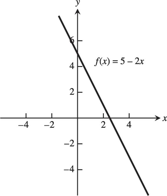
17. The domain is (,).
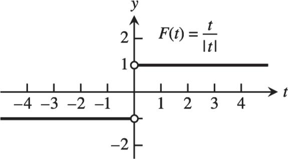
19. The domain is (,0)(0,).
21. The domain is (,5)(5,3][3,5)(5,).
23. Neither graph passes the vertical line test.
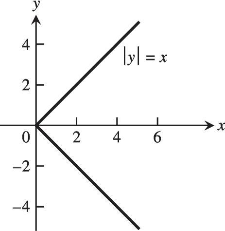
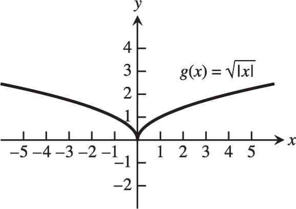
16. The domain is (,).
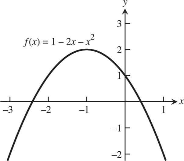
18. The domain is (,0].
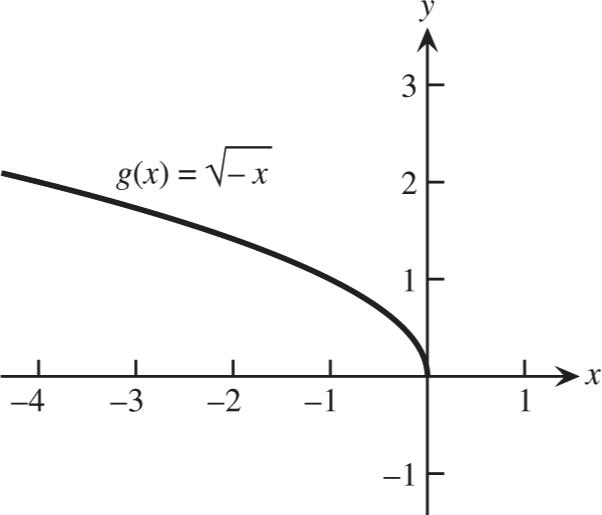
20. The domain is (,0)(0,).
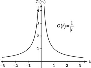
22. The range is [5,) .
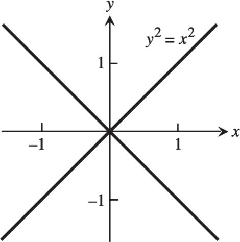
24. Neither graph passes the vertical line test. (a) (b)
012 010 x y
012 100 x y 27. 2 2 4,1 () 2,1 x x F x x xx
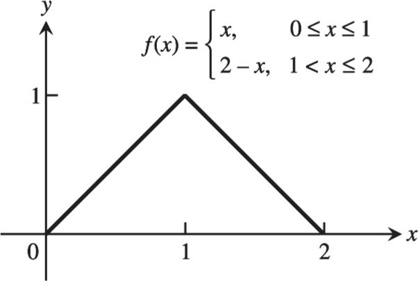
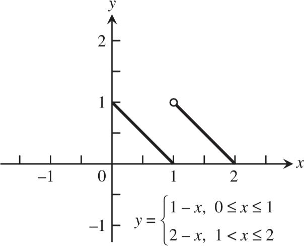
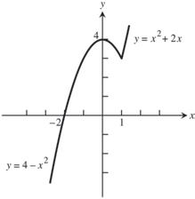
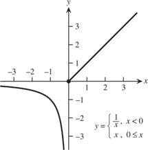
29. (a) Line through (0, 0) and (1, 1): ; y x Line through (1, 1) and (2, 0): 2 y x ,01 () 2,12 x x fx x x
(b) 2,01 0,12 () 2,23 0,34 x x fx x x
30. (a) Line through (0, 2) and (2, 0): 2 y x Line through (2, 1) and (5, 0): 01 11 5233 , m so 5 11 333 (2)1 y xx
5 1 33 2,02 () ,25 xx fx xx
1 Functions
(b) Line through (1,0) and (0,3): 30 0(1) 3, m so 33 y x
Line through (0, 3) and 13 4 202 (2,1): 2, m so 23 y x 33,10 () 23,02 x x fx x x
31. (a) Line through (1,1) and (0, 0): y x
Line through (0, 1) and (1, 1): 1 y
Line through (1, 1) and (3, 0): 01 11 3122 , m so 3 11 222 (1)1 y xx
3 1 22 10 ()101 13 x x fxx x x
(b) Line through (2,1) and (0, 0): 1 2 y
Line through (0, 2) and (1, 0): 22 y x
Line through (1,1) and (3,1): 1 y
32. (a) Line through 2 ,0 T and (T, 1): 10 2 (/2) , TTT m
33. (a) 0for[0,1)xx
only when x is an integer.
35. For any real number ,1,x nxn where n is an integer. Now: 1(1). nxnnxn
By definition: and
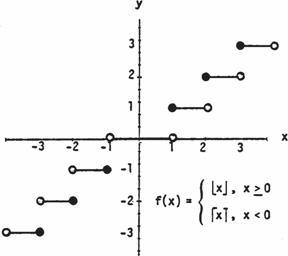
36. To find f (x) you delete the decimal or fractional portion of x, leaving only the integer part.
for all
Copyright 2023 Pearson Education, Inc.
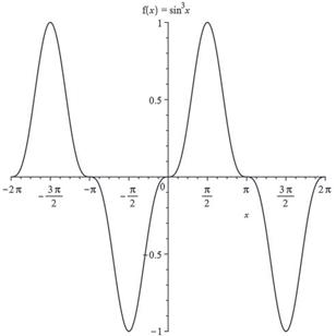
37. Symmetric about the origin
Dec: x
Inc: nowhere
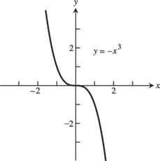
39. Symmetric about the origin
Dec: nowhere
Inc: 0 0 x x
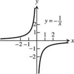
41. Symmetric about the y-axis
Dec: 0 x
Inc: 0 x
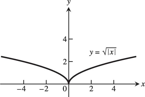
38. Symmetric about the y-axis
Dec: 0 x
Inc: 0 x
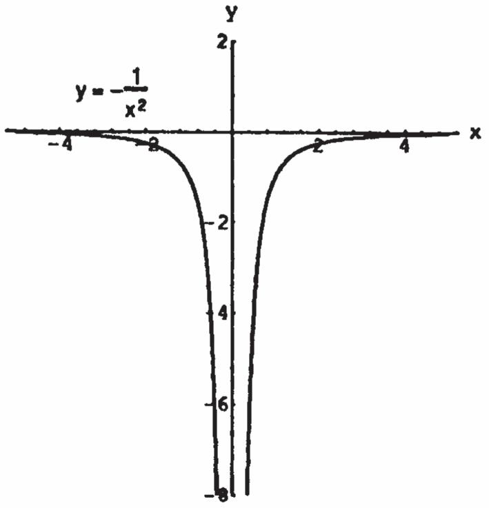
40. Symmetric about the y-axis
Dec: 0 x
Inc: 0 x
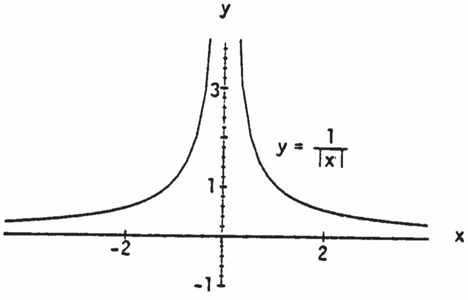
42. No symmetry
Dec: 0 x
Inc: nowhere
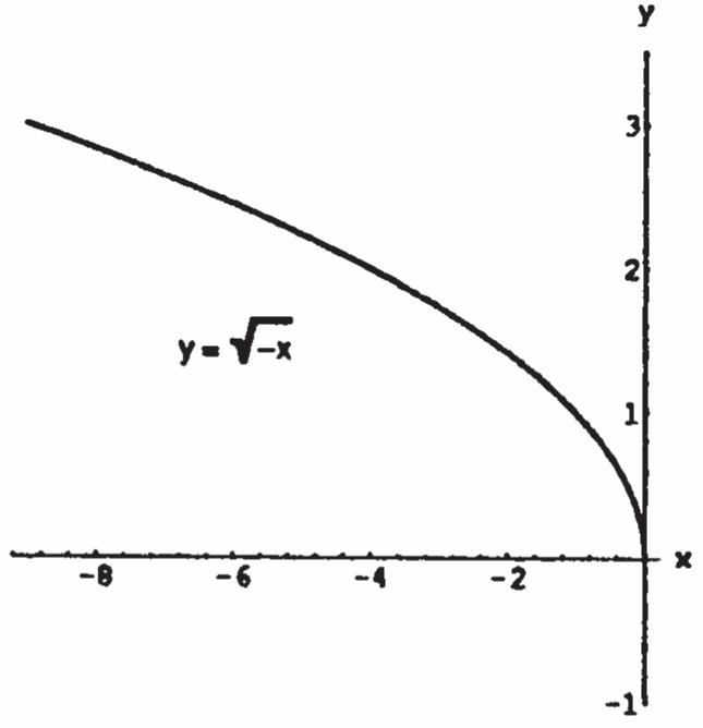
43. Symmetric about the origin
Dec: nowhere
Inc: x
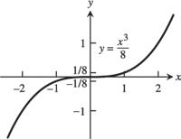
45. No symmetry
Dec: 0 x
Inc: nowhere
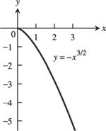
44. No symmetry
Dec: 0 x
Inc: nowhere
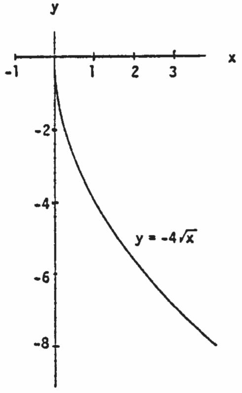
46. Symmetric about the y-axis
Dec: 0 x
Inc: 0 x
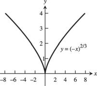
47. Since a horizontal line not through the origin is symmetric with respect to the y-axis, but not with respect to the origin, the function is even.
48. 55 5 55111 () ()and()() (). xx x f xxfxx fx Thus the function is odd.
49. Since 22 ()1()1(). f xxxfx The function is even.
50. Since 22 [ ()][()()] f xxxfxxx and 22 [ ()][()()] f xxxfxxx the function is neither even nor odd.
51. Since (),()333()() g xxxgxxxxxgx So the function is odd.
52. 4242 ()31()3()1(), g xxxxxgx thus the function is even.
53. 22 11 1()1 () (). xx g xg x Thus the function is even.
54. ();()2211 (). x x xx g xgxgx So the function is odd.
55. 111 ();();()111 ttt hththt Since ()()and()(), hthththt the function is neither even nor odd.
56. Since 33 |||()|,()() tththt and the function is even.
57. ()21,()21. htthtt So ()().()21, hththtt so ()().htht The function is neither even nor odd.
58. ()2||1and()2||12||1. htthttt So ()() htht and the function is even.
59. ()sin2;()sin2(). g xxgxxgx So the function is odd.
60. 22 ()sin;()sin(). g xxgxxgx So the function is even.
61. ()cos3;()cos3(). g xxgxxgx So the function is even.
62. ()1cos;()1cos(). g xxgxxgx So the function is even.
63. 111 333 25(75) ;60180sktkksttt
64. 2222 12960(18)4040;40(10)4000joulesKcvccKvK
65. 242412 624;1045kk sss rkrs
66. 3 147001470024500 100039 14.7 14700 ;23.4 628.2in. kk VVV PkPV
67. 32 ()(142)(222)472308;07 Vfxxxxxxxx
68. (a) Let h height of the triangle. Since the triangle is isosceles, 22 2 22.ABABAB So,
2 22121 hhB is at (0,1) slope of 1 AB The equation of AB is ()1;[0,1].yfxxx (b) 2 ()22(1) [0, 2] ;1 2 Axxyxxxx x
69. (a) Graph h because it is an even function and rises less rapidly than does Graph g.
(b) Graph f because it is an odd function.
(c) Graph g because it is an even function and rises more rapidly than does Graph h.
70. (a) Graph f because it is linear.
(b) Graph g because it contains (0, 1).
(c) Graph h because it is a nonlinear odd function.
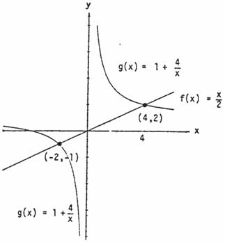
71. (a) From the graph, 4 2 1(2,0)(4,) x x x
(b) 44 22110 x x x x 2 28(4)(2) 4 0:10222 0 0 xxxx x x xx x
4 x since x is positive; 2 28(4)(2) 4 0:10222 0 0 xxxx x x xx x
2 x since x is negative; sign of (4)(2) x x

Solution interval: (2,0)(4,)
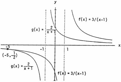
72. (a) From the graph, 3 2 11 (,5)(1,1) xx x
(b) Case 1: x 3(1) 3 2 111 2 x xxx 33225. x xx Thus, (,5) x solves the inequality.
Case 11: x 3 2 11xx 3(1) 1 2 x x 33225 x xx which is true if 1. x Thus, (1,1) x solves the inequality.
Case 1 : x 3 2 11 3 xx x 3 22 x 5 x which is never true if 1 ,x so no solution here.
In conclusion, (,5)(1,1). x
73. A curve symmetric about the x-axis will not pass the vertical line test because the points (x, y) and (,) x y lie on the same vertical line. The graph of the function () 0 y fx is the x-axis, a horizontal line for which there is a single y-value, 0, for any x.
74. price405, x quantity 30025 x () R x (405)(30025) x x
76. (a) Note that 2mi10,560ft, so there are 80022 x feet of river cable at $180 per foot and (10,560) x feet of land cable at $100 per foot. The cost is ()18080022 Cxx
100(10,560 - x). (b) (0)$1,200,000 (500)$1,175,812 (1000)$1,186,512 (1500)$1,212,000 (2000)$1,243,732 (2500)$1,278,479 (3000)$1,314,870
Values beyond this are all larger. It would appear that the least expensive location is less than 2000 feet from the point P
1.
2.
3.
5. (a) 2 (b)
(d) 22 (5)31022 xxx
(g) 10 x (h) (3)362242 6 xxx
6. (a) 1 3 (b) 2 (c) 1 11 1 x xx (d)
7. ()()((())) f ghxfghx
((4)) f gx
8. 2 ()()((()))(()) fghxfghxfgx
9.
1 ()()((())) x fghxfghxfg
10.
()()((()))2 fghxfghxfgx
(3(4)) f x (123)(123) f xx
11. (a) ()() f gx (b) ()() j gx (c) ()() g gx (d) ()() j jx (e) ()() g hfx
12. (a) ()() f jx
(d) ()() f fx
(b) ()() g hx
(e) ()() j gfx
13. g(x) f (x) ()() f gx (a) 7 x x 7 x (b) 2 x 3x 3(2)36 x x (c) 2 x 5 x 2 5 x (d) 1 x x 1 x x 1 1 (1) 1 x x x x x xx x (e) 1 1 x 1 1 x
(f ) ()() hjfx
(c) ()() hhx
(f ) ()() g fhx
14. (a) 1 1 ()()|()| x fgxgx
(b) ()1 ()1 ()() g x x gxx fgx
(c) Since ()()()||, f gxgxx 2 (). g xx
(d) Since ()()||, f gxfxx 2 (). f xx (Note that the domain of the composition is [0,). )
The completed table is shown. Note that the absolute value sign in part (d) is optional.
x
15. (a) ((1))(1)1 f gf (b) ((0))(2)2 g fg
(c) ((1))(0)2 f ff (d) ((2))(0)0 g gg (e) ((2))(1)1 g fg
(f) ((1))(1)0 f gf
16. (a) ((0))(1)2(1)3, f gf where (0)011 g
(b) ((3))(1)(1)1, g fg
where (3)231 f
(c) ((1))(1)110, g gg where (1)(1)1 g
(d) ((2))(0)202, f ff where (2)22 0 f
(e) ((0))(2)211, g fg where (0)202 f
(f )
5 111 2222 2, fgf
17. (a) 1 1 ()()(())1 x x x fgxfgx
1 1 ()()(()) x gfxgfx (b) Domain ():(,1](0,), f g
18. (a) ()()(())12 f gxfgxxx
()()(())1|| g fxgfxx
Domain
()()(()) f gxxfgxx
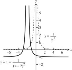
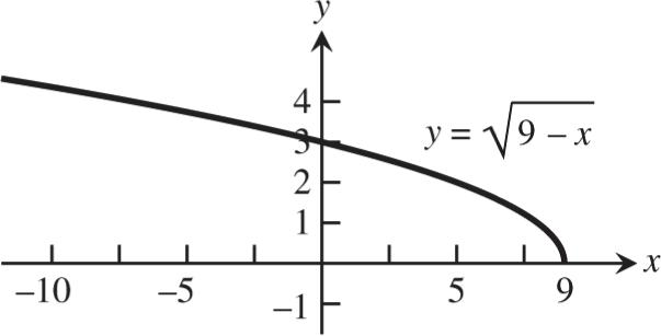
Copyright 2023 Pearson Education, Inc.
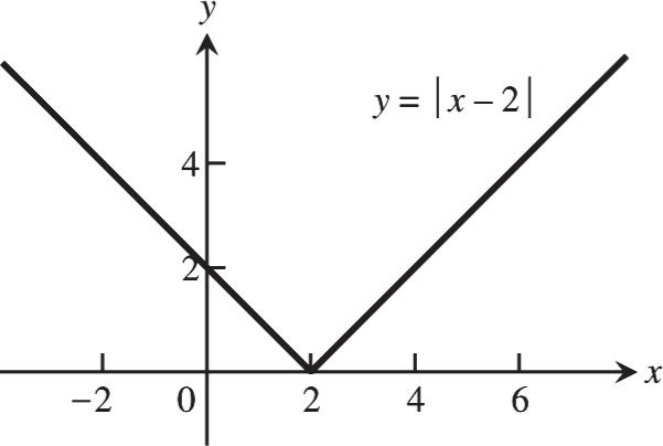
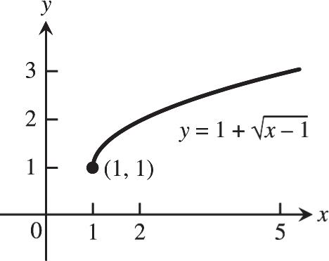
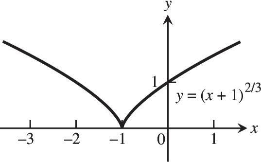
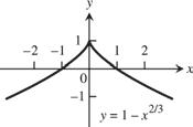
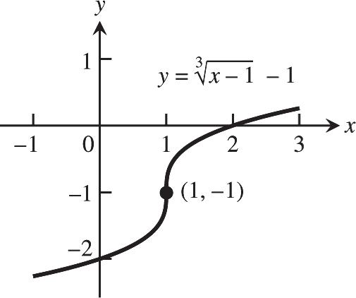
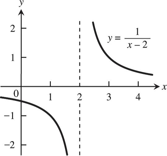
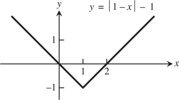
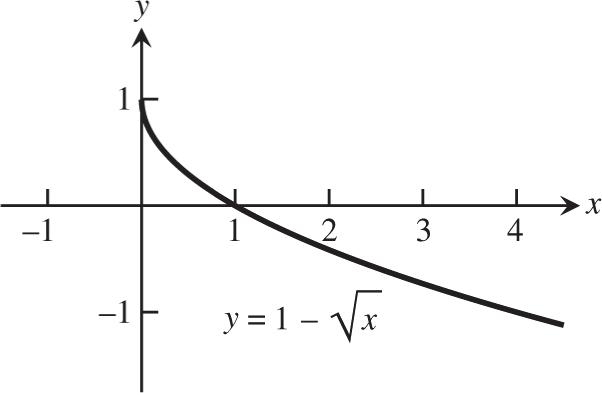
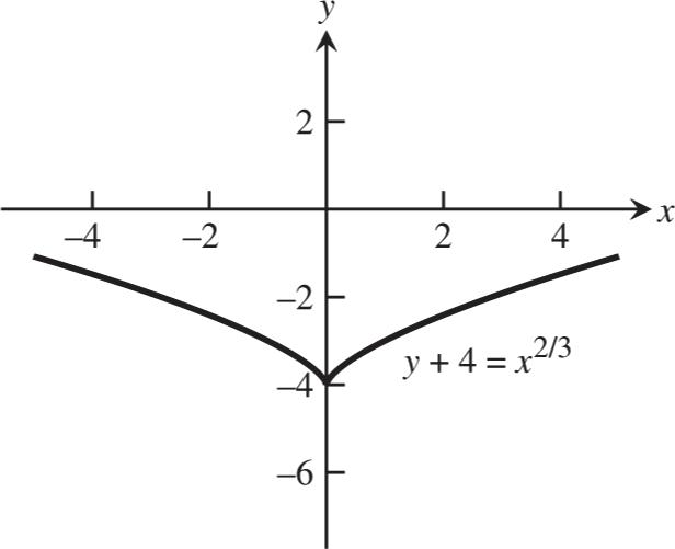
Copyright 2023 Pearson Education, Inc.
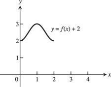
57. (a) domain: [0, 2]; range: [2, 3]
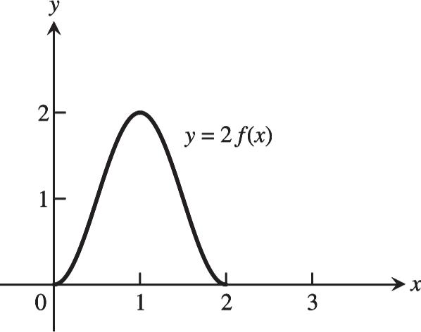
(c) domain: [0, 2]; range: [0, 2]
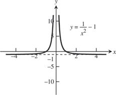
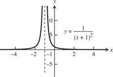
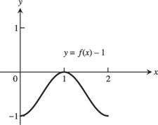
(b) domain: [0, 2]; range: [–1, 0]
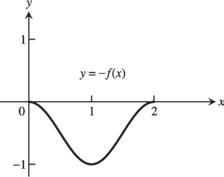
(d) domain: [0, 2]; range: [–1, 0]
Copyright 2023 Pearson Education, Inc.
(e) domain: [–2, 0]; range: [0, 1]
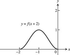
(g) domain: [–2, 0]; range: [0, 1]
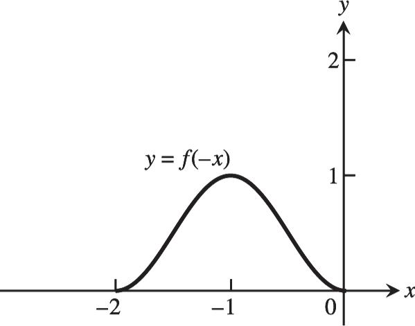
58. (a) domain: [0, 4]; range: [–3, 0]
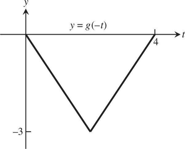
(c) domain: [–4, 0]; range: [0, 3]
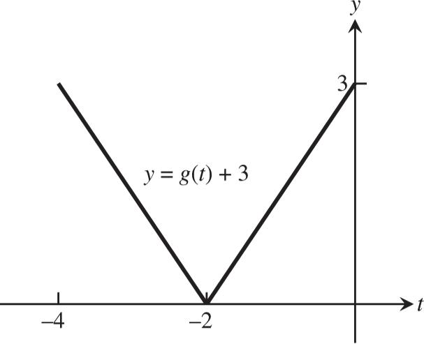
(e) domain: [2, 4]; range: [–3, 0]
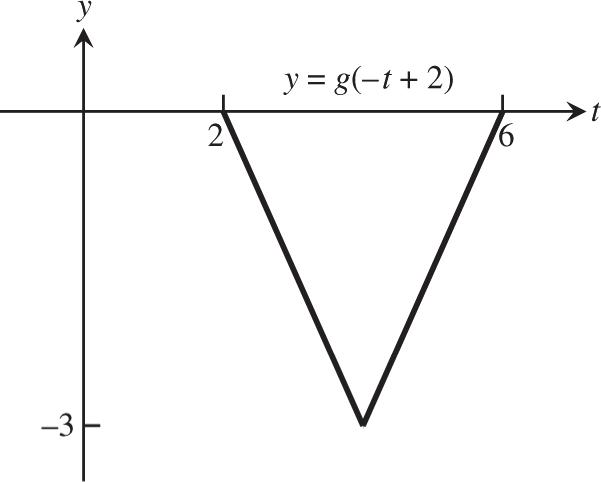
(f ) domain: [1, 3]; range: [0,1]
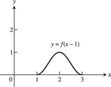
(h) domain: [–1, 1]; range: [0, 1]
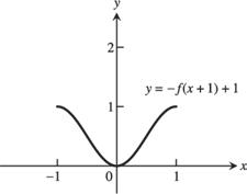
(b) domain: [–4, 0]; range: [0, 3]
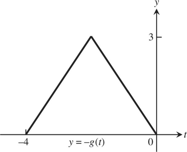
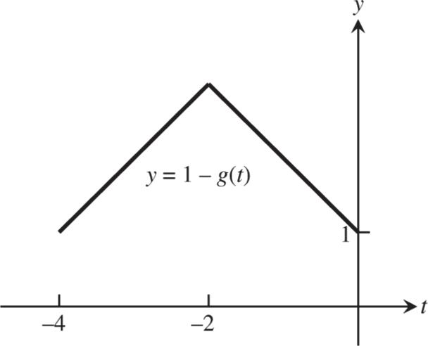
(d) domain: [–4, 0]; range: [1, 4]
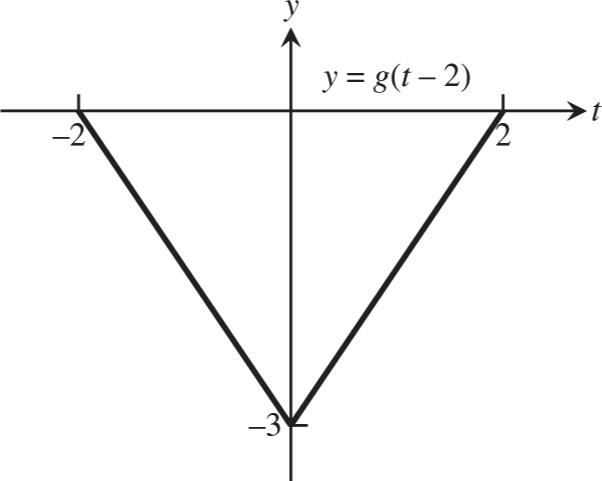
(f ) domain: [–2, 2]; range: [–3, 0]
Copyright 2023 Pearson Education, Inc.
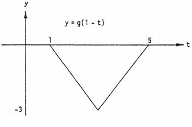
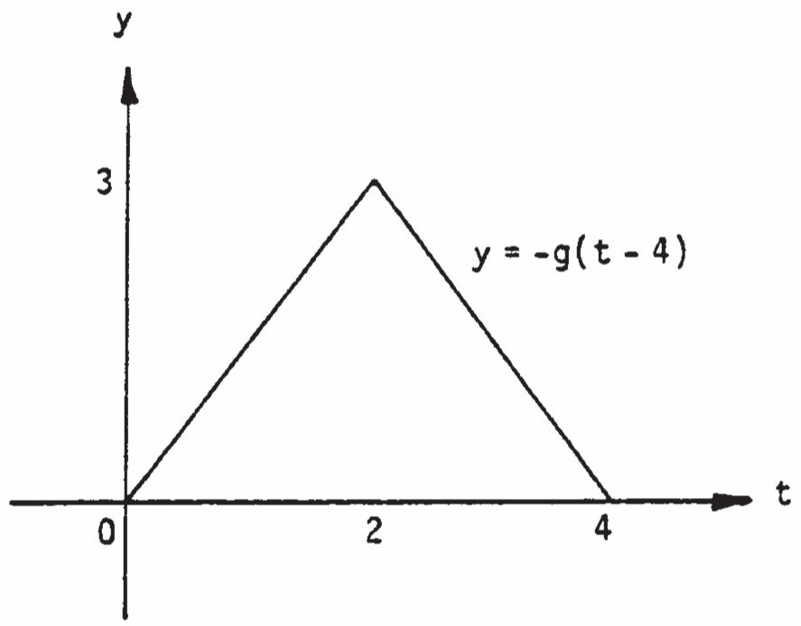
(g) domain: [1, 5]; range: [–3, 0] (h) domain: [0, 4]; range: [0, 3] 59. 2 33yx
22 (2)141yxx
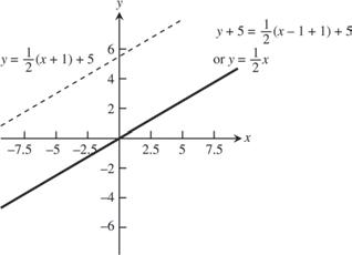
63. 41 y x
2 2 1 22 416 x y x
67. 1(3)12733 y xx
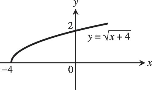
69. Let 21() y xfx and let 1/2 (), g xx
1/2 1 2 (),hxx
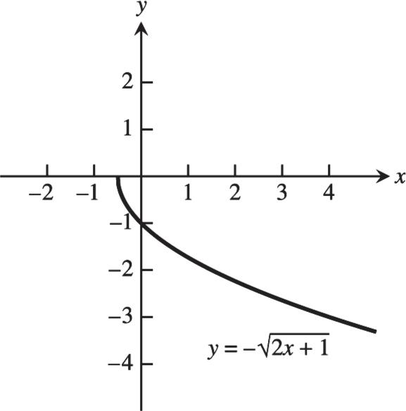
1/2 1 2 ()2, ixx and 1/2 1 2 ()2 ().jxxfx The graph of ()hx is the graph of () g x shifted left 1 2 unit; the graph of () i x is the graph of ()hx stretched vertically by a factor of 2; and the graph of ()() jxfx is the graph of () i x reflected across the x-axis.
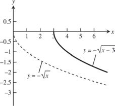
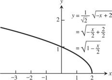
70. Let 2 1(). x y fx Let () g x 1/2 (), x ()hx 1/2 (2), x and 1/2 1 2 ()(2) ixx
2 1(). x f x The graph of () g x is the graph of y x reflected across the x-axis. The graph of ()hx is the graph of () g x shifted right two units. And the graph of () i x is the graph of ()hx compressed vertically by a factor of 2 .
31 y x
2 1 3 4 y x
Copyright 2023 Pearson Education, Inc.
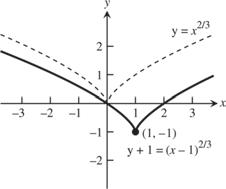
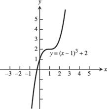
71. 3 (). y fxx Shift () f x one unit right followed by a shift two units up to get 3 ()(1)2gxx .
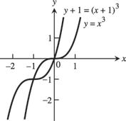
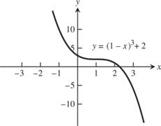
72. 33 (1)2[(1)(2)](). yxxfx
Let 33 (),()(1), gxxhxx 3 ()(1)(2), ixx and ()[(1)3 jxx (2)]. The graph of ()hx is the graph of () g x shifted right one unit; the graph of () i x is the graph of ()hx shifted down two units; and the graph of () f x is the graph of () i x reflected across the x-axis.
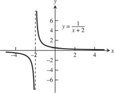
73. Compress the graph of 1 () x fx horizontally by a factor of 2 to get 1 2 () x gx Then shift () g x vertically down 1 unit to get 1 2 ()1. x hx
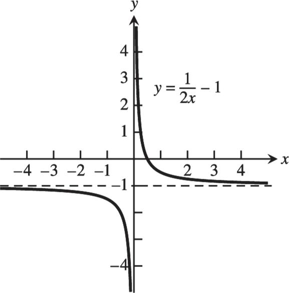
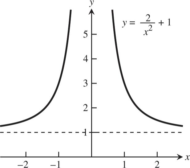
74. Let 2 1 () x fx and 2 2 2 21 ()11 x x gx
Since 21.4, we see that the graph of () f x stretched horizontally by a factor of 1.4 and shifted up 1 unit is the graph of () g x .
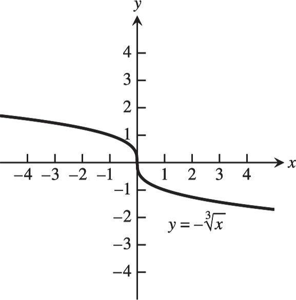
75. Reflect the graph of 3 () y fxx across the x-axis to get 3 (). g xx
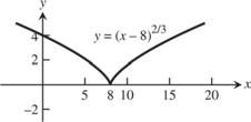
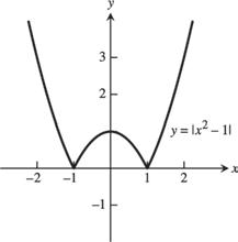
76. 2/3 ()(2)[(1)(2)](1)(2)2/32/32/3 yfxxxx 2/3 (2). x So the graph of () f x is the graph of 2/3 () g xx compressed horizontally by a factor of 2.
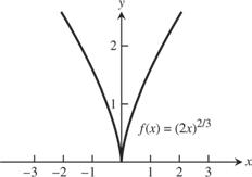
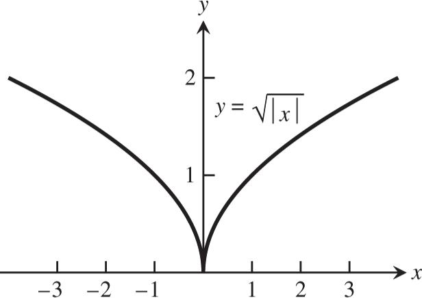
79. (a) ()()()()()(()) fgxfxgxfxgx ()(), fgx odd
(b)
(c)
()() ()() () (), ffxfxf ggxgxg x x odd
()() ()() () (), ggxgxg ffxfxf x x odd
(d) 22 ()()()()()(), f xfxfxfxfxfx even
(e) 222 2 ()(())(())(), g xgxgxgx even
(f ) ()()(())(()) f gxfgxfgx
(g) ()()(())(()) g fxgfxgfx
(h) ()()(())(()) f fxffxffx
(i) ()()(())(()) g gxggxggx
(())()(), f gxfgx
even
()(), g fx even
f fx
even
(()) g gx ()(), g gx
odd
80. Yes, ()0 f x is both even and odd since ()0() f xfx and ()0() f xfx .
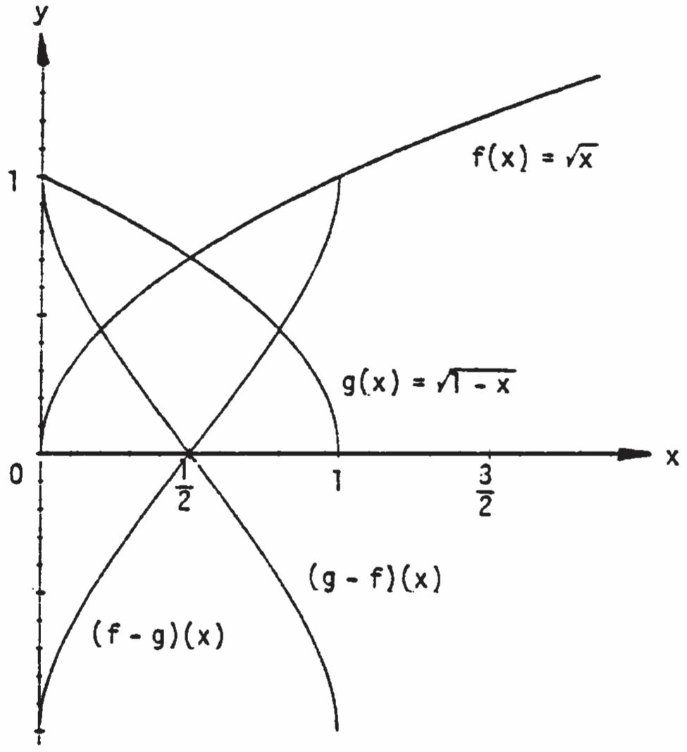
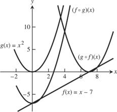
81. (a) (b)
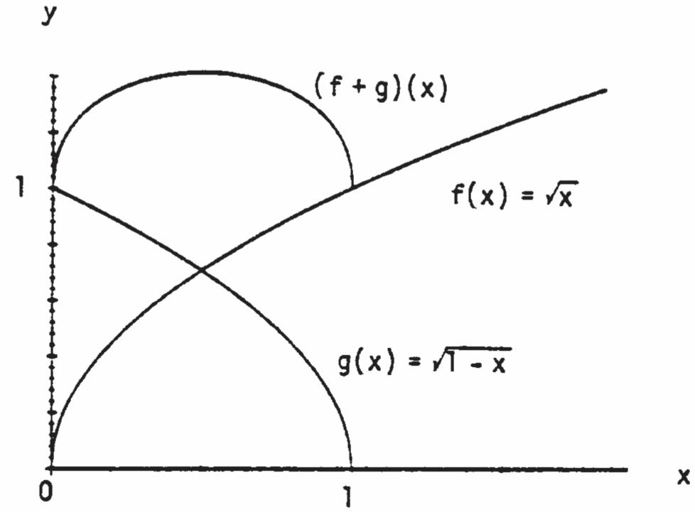
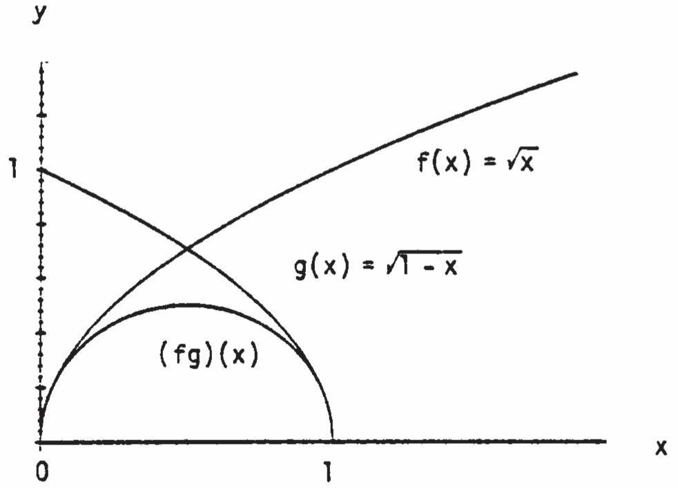
1.3 TRIGONOMETRIC FUNCTIONS
1.
2.
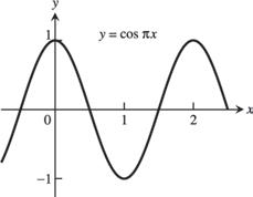
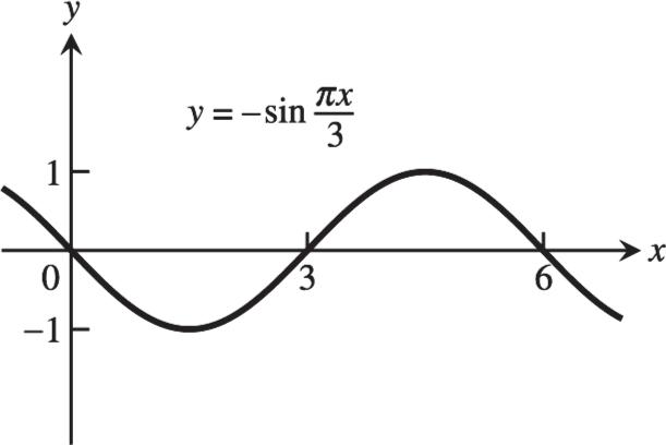
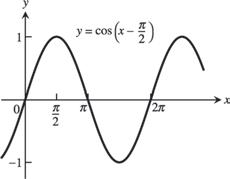
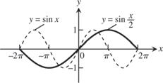
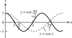
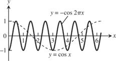
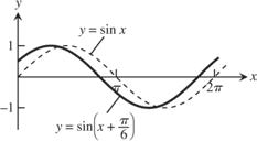
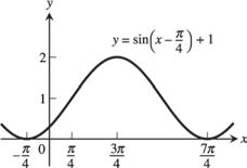
period2 22. period2
23. 2 period, symmetric about the origin
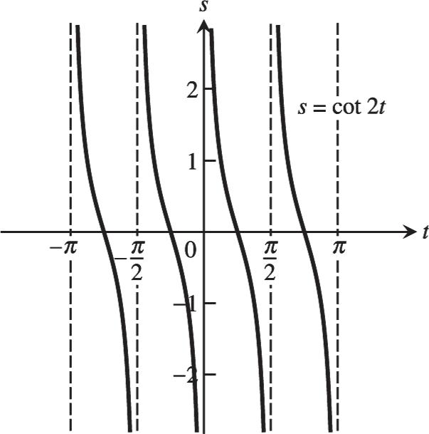
25. period4, symmetric about the s-axis
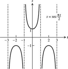
27. (a) cos x and sec x are positive for x in the interval 22,; and cos x and sec x are negative for x in the intervals 3 22 , and 3 22 , sec x is undefined when cos x is 0. The range of sec x is (,1][1,); the range of cos x is [ 1,1].
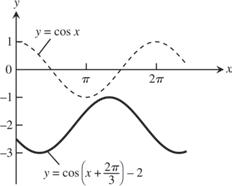
24. period1, symmetric about the origin
26. period4, symmetric about the origin
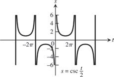
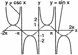
(b) sin x and csc x are positive for x in the intervals 3 2 , and (0,); and sin x and csc x are negative for x in the intervals (,0) and 3 2 , . csc x is undefined when sin x is 0. The range of csc x is (,1][1,); the range of sin x is [ 1,1].
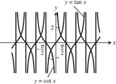
28. Since 1 tan cot, x x cot x is undefined when tan 0 x and is zero when tan x is undefined. As tan x approaches zero through positive values, cot x approaches infinity. Also, cot x approaches negative infinity as tan x approaches zero through negative values. 29.
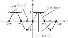
33. 222 sinsincoscossin(sin)(0)(cos)(1)cos x xxxxx
34. 222 sinsincoscossin(sin)(0)(cos)(1)cos x xxxxx
35. cos()cos(())coscos()sinsin()coscossin(sin) coscossinsin A BABABABABAB A BAB
36. sin()sin(())sincos()cossin()sincoscos(sin) sincoscossin A BABABABABAB A BAB
37. If , 0cos()cos01. B AABAB Also cos()cos()cos A BAA cos A A sin A sin A 22 cossin. A A Therefore, 2 cos A 2 sin1. A
38. If 2, B then cos(2) A coscos2 A sinsin2(cos)(1) A A (sin)(0)cos A A and sin(2)sincos2cossin2(sin)(1)(cos)(0)sin A AAAAA . The result agrees with the fact that the cosine and sine functions have period 2.
39. cos()coscossinsin(1)(cos)(0)(sin)cos x xxxxx
40. sin(2)sin2cos()cos(2)sin()(0)(cos())(1)(sin())sin x xxxxx
41.
333 222 sinsincos()cossin()(1)(cos)(0)(sin())cos x
42.
43.
333 222 coscoscossinsin(0)(cos)(1)(sin)sin x
62 3 22 7 1 1243434322224 sinsinsincoscossin
26 3 22 11222 1 1243434322224 coscoscoscossinsin
52.
53. sin2cos02sincoscos0 cos(2sin1)0cos0 or 2sin10 3 1 222 cos0 or sin ,,or
55 3 666262 ,,,,
54. 2 cos2cos02cos1cos0 2 2coscos10(cos1)(2cos1)0
cos10or2cos1 1 2 0cos1orcos or 55 3333 ,,,
55. sincoscossin coscoscoscos coscossinsin coscoscoscos sin()sincoscoscos tantan cos()coscossinsin 1tantan tan() ABAB ABAB ABAB ABAB A BABAB AB A BABAB AB AB
56. sincoscossin coscoscoscos coscossinsin coscoscoscos sin()sincoscoscos tantan cos()coscossinsin 1tantan tan()
ABAB ABAB ABAB ABAB A BABAB AB A BABAB AB AB
57. According to the figure in the text, we have the following: By the law of cosines, 222 2coscabab 22 112cos()22cos() A BAB . By distance formula, 222 (coscos)(sinsin) cABAB 22 22 cos2coscoscossin2sinsinsin22(coscossinsin) A ABBAABBABAB . Thus 2 22cos()22(coscossinsin)cos()coscossinsin cABABABABABAB .
58. (a) cos()coscossinsin A BABAB
sincosandcossin22 Let A B
sin()cos()cos2222coscossinsin sincoscossin A BABABABAB A BAB
Because the cosine function is even and the sine function is odd.
(b) cos()coscossinsin cos(())coscos()sinsin() cos()coscos()sinsin()coscossin(sin)coscossinsin
ABABAB ABABAB A BABABABABABAB
59. 222 22 2cos232(2)(3) c ababC
1 2 cos(60)4912cos(60)13127 Thus, 72.65. c
60. 222 22 2cos232(2)(3) c ababC cos(40)1312cos(40). Thus, 1312cos40°1.951. c
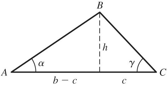
61. From the figures in the text, we see that sin . h c B If C is an acute angle, then sin. h b C On the other hand, if C is obtuse (as in the figure on the right in the text), then sin C sin() . h b C Thus, in either case, sinsin sinsin. hbCcBahabCacB
By the law of cosines, 222 2 cos abc ab C and 222 2 cos . acb ac B Moreover, since the sum of the interior angles of triangle is , we have sin A sin(()) BC sin() BC sincosBC cossinBC
222 2 abc h cab
222 2 acb h acb
22222 2 (2 ) h abc abccb ah bc ah sin. bcA
Combining our results we have ahab sin C, ahac sin B, and ahbc sin A. Dividing by abc gives sinsinsin law of sines A CB h bcacb
62. By the law of sines, 3/2 sinsin 23 AB c By Exercise 59 we know that 7. c Thus 33 27 sin0.982. B
63. From the figure at the right and the law of cosines, 222 22 1 2 22(2)cos 4424. b aaB aaaa
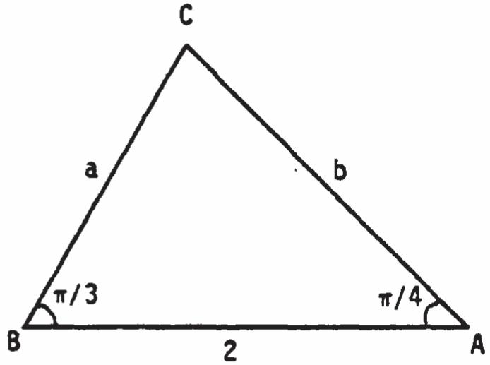
Applying the law of sines to the figure, sinsin A B ab 2/23/2 3 2 ab ba Thus, combining results, 22 24 aab 22 3 1 22 0 aa 2 24048 aaa . From the quadratic formula and the fact that 0, a we have 2 444(1)(8) 434 22 1.464. a
64.
tan hh
tantantantan
tantantantan
tantan(tantan)
65. sin
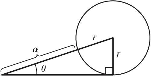
66. (a) The graphs of sin y x and y x nearly coincide when x is near the origin (when the calculator is in radians mode).
(b) In degree mode, when x is near zero degrees the sine of x is much closer to zero than x itself. The curves look like intersecting straight lines near the origin when the calculator is in degree mode. 67. 2,2,,1 A
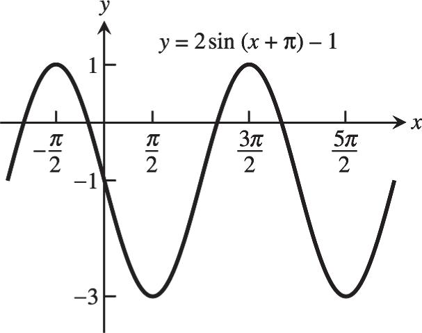
68. 11 22 ,2,1, ABCD
69. 21 ,4,0, ABCD
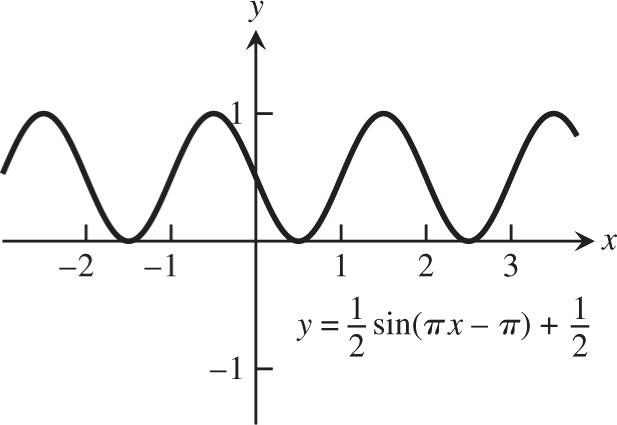
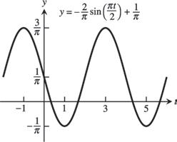
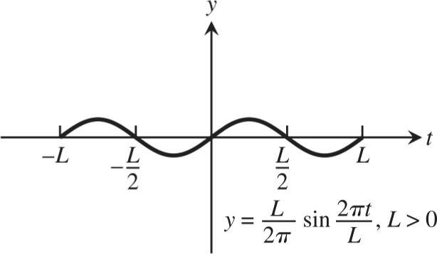
71–74. Example CAS commands: Maple:
f :x-A*sin((2*Pi/B)*(x-C))D1; A:3; C:0; D1:0; f_list :[seq(f(x), B[1,3,2*Pi,5*Pi])]; plot(f_list, x-4*Pi..4*Pi, scalingconstrained, color[red,blue,green,cyan], linestyle[1,3,4,7],
legend["B1", "B3","B2*Pi","B3*Pi"], title"#71 (Section 1.3)");
Mathematica: Clear[a, b, c, d, f, x] f[x_]:a Sin[2/b(xc)]d Plot[f[x]/.{a3, b1, c0, d0},{x,4, 4}]
71. (a) The graph stretches horizontally.
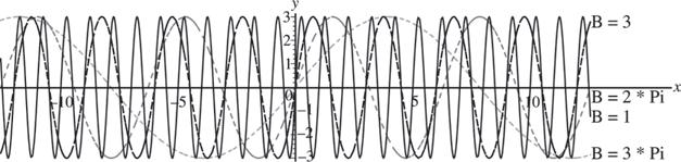
(b) The period remains the same: period || B . The graph has a horizontal shift of 1 2 period.
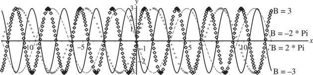
72. (a) The graph is shifted right C units.
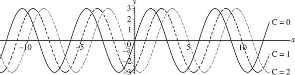
(b) The graph is shifted left C units.
(c) A shift of one period will produce no apparent shift. ||6 C
73. (a) The graph shifts upwards || D units for 0. D (b) The graph shifts down || D units for 0. D
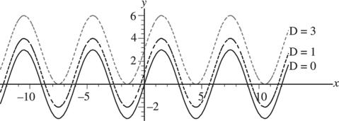
74. (a) The graph stretches || A units. (b) For 0, A the graph is inverted.
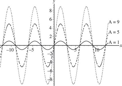
1–4. The most appropriate viewing window displays the maxima, minima, intercepts, and end behavior of the graphs and has little unused space.
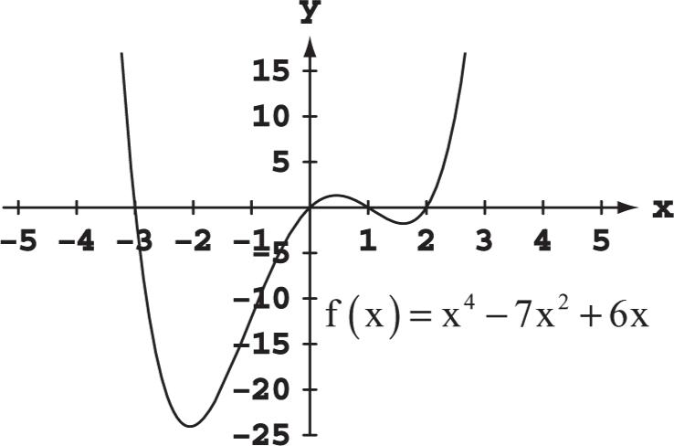
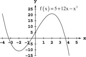
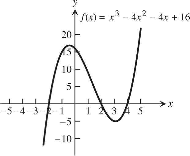
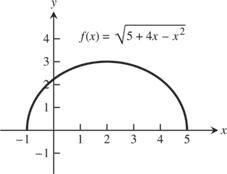
5–30. For any display there are many appropriate display widows. The graphs given as answers in Exercises 5–30 are not unique in appearance.
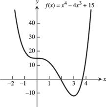
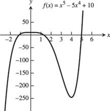
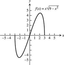
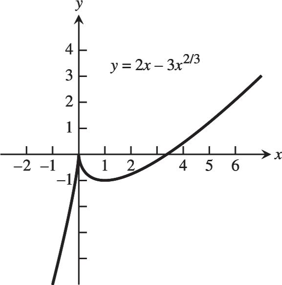
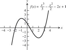
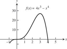
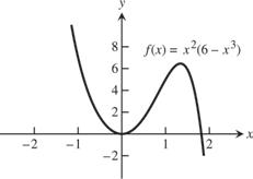
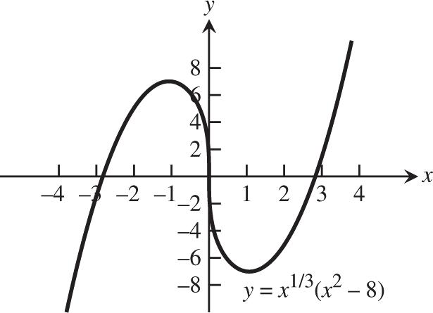
Copyright 2023 Pearson Education, Inc.
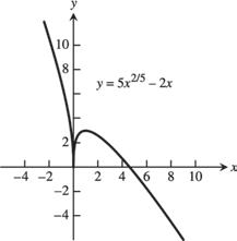
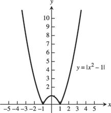
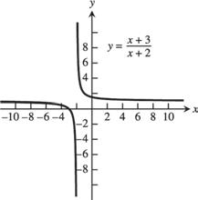
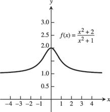
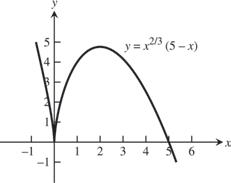
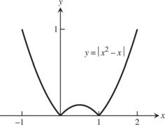
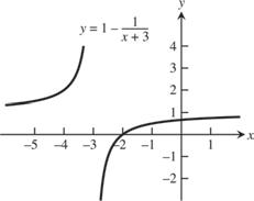
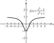
21. [10, 10] by [6, 6]
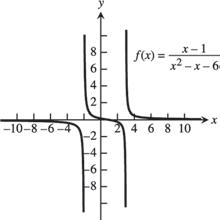
23. [6, 10] by [6, 6]
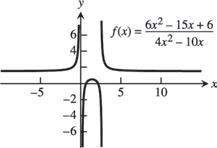
25. [0.03,0.03] by [1.25,1.25]
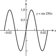
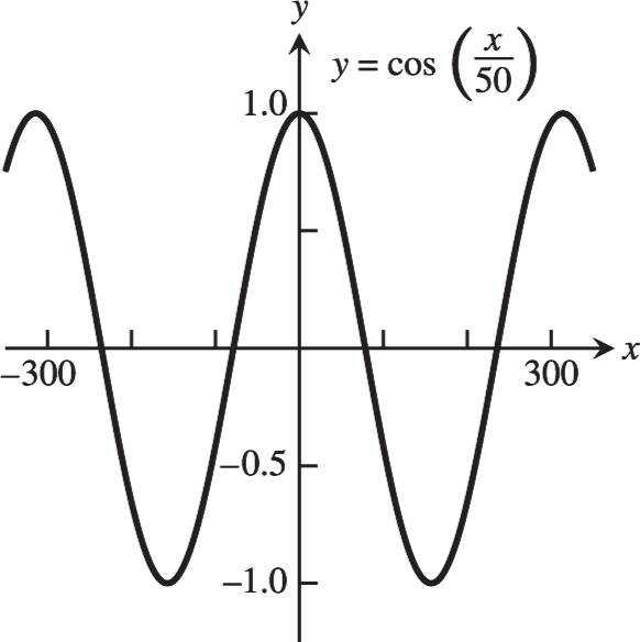
27. [300,300]by[1.25,1.25]
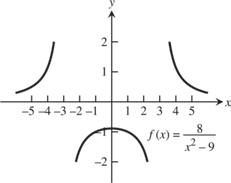
22. [5, 5] by [2, 2]
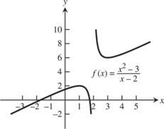
24. [3, 5] by [2, 10]
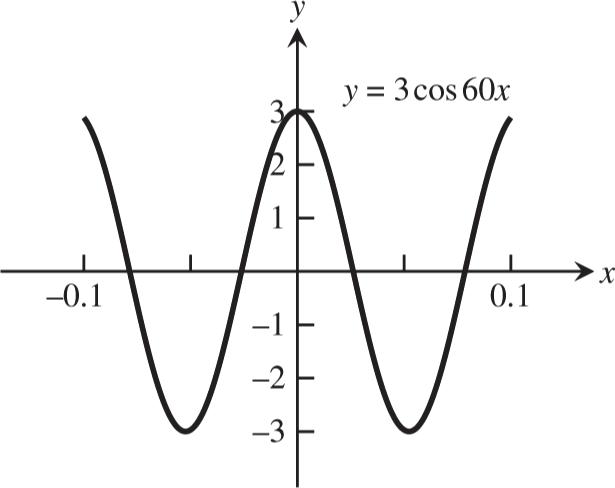
26. [0.1,0.1]by[3,3]
28. [50,50]by[0.1,0.1]
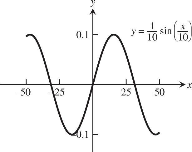
29. [0.25,0.25]by[0.3,0.3]
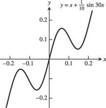
31. 22 244 x xyyy 2 228. xx The lower half is produced by graphing 2 228.yxx
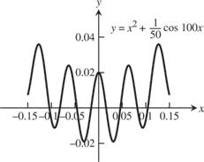
30. [0.15,0.15]by[0.02,0.05]
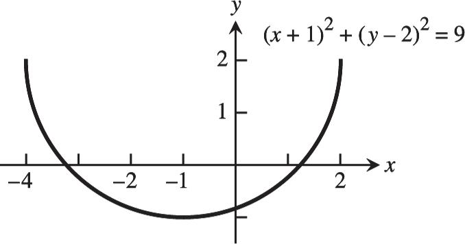
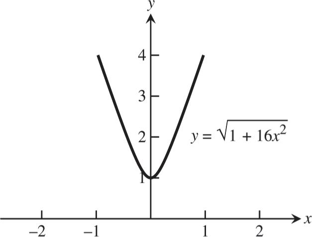
32. 22 2 161116. yxyx The upper branch is produced by graphing 2 116. y x
1. The area is 2 A r and the circumference is 2.Cr Thus, 2 2 224 rACCC
2. The surface area is 1/2 2 4 4. S Srr The volume is 3 3 4 3 34 . V Vrr Substitution into the formula for surface area gives 2/3 2 3 4 44. V Sr
3. The coordinates of a point on the parabola are (x, x2). The angle of inclination joining this point to the origin satisfies the equation 2 tan. x x x Thus the point has coordinates 2 (,) xx 2 (tan,tan)
4. rise run500 tan 500tanft h h
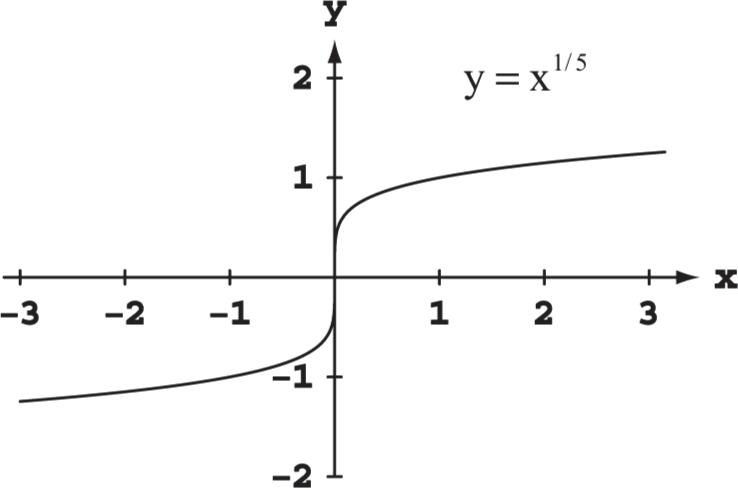
Symmetric about the origin
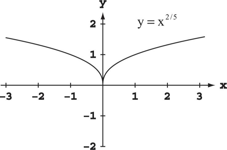
Symmetric about the y-axis
Symmetric about the y-axis
16. ()()cos()cos(); yxxxxxyx odd
17. Since f and g are odd ()() f xfx and ()(). g xgx
(a) ()()()() f gxfxgx [()] f x [()] gx ()()()() f xgxfgxfg is even.
(b) 3 ()()()() f xfxfxfx [()] f x [] f x [()] fx
(c) (sin())(sin()) fxfx (sin())fx (sin()) f x is odd.
(d) (sec())(sec())(sec()) g xgxgx is even.
(e) |()||()||()||| g xgxgxg is even.
()()() f xfxfx 33 () f xf is odd.
18. Let ()() f axfax and define () g x (). f xa Then ()(()) g xfxa ()() f axfax ()()()() f xagxgxfxa is even.
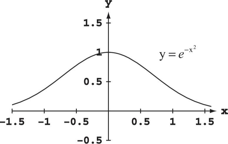
19. (a) The function is defined for all values of x, so the domain is (,)
(b) Since || x attains all nonnegative values, the range is [2,)
20. (a) Since the square root requires 10 x , the domain is (,1]
(b) Since 1 x attains all nonnegative values, the range is [2,)
21. (a) Since the square root requires 2 160, x the domain is [4,4] .
(b) For values of x in the domain, 2 01616, x so 2 0164. x The range is [0,4]
22. (a) The function is defined for all values of x, so the domain is (,)
(b) Since 32 x attains all positive values, the range is (1,)
23. (a) The function is defined for all values of x, so the domain is (,) .
(b) Since 2 x e attains all positive values, the range is (3,)
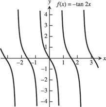
24. (a) The function is equivalent to tan2, y x so we require 2 2 k x for odd integers k. The domain is given by 4 k x for odd integers k
(b) Since the tangent function attains all values, the range is (,)
25. (a) The function is defined for all values of x, so the domain is (,).
(b) The sine function attains values from –1 to 1, so 22sin(3)2 x and hence 32sin(3)11. x The range is [3,1].
26. (a) The function is defined for all values of x, so the domain is (,).
(b) The function is equivalent to 5 2 , yx which attains all nonnegative values. The range is [0,)
27. (a) The function is defined for all values of x, so the domain is (,).
(b) The cosine function attains values from –1 to 1, so 1cos31 x and hence 0cos312. x The range is 0,2.
28. (a) The function is defined for all values of x, so the domain is (,). (b) The cube root attains all real values, so the range is (,).
29. 5(3)(1)yxx so the domain(,1][3,); (3)(1)0 xx and can be any positive number, so the range(,5].
30. 2 2 3 4 2 x x y so the domain(,); 2 2 3 4 03 x x so the range[2,5).
31. 1 4sin x y so the domain(,0)(0,); if 22 3 , x then 1 1sin1, x so the range[4,4].
32. 3cos4sin yxx so the domain(,); and 22 345 so 3 4 55 3cos4sin5cossin x xxx 5(coscossinsin )5cos(), x xx where and 1cos()1 x so the range[5,5].
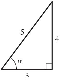
33. (a) Increasing because volume increases as radius increases (b) Neither, since the greatest integer function is composed of horizontal (constant) line segments. (c) Decreasing because as the height increases, the atmospheric pressure decreases. (d) Increasing because the kinetic (motion) energy increases as the particles velocity increases.
34. (a) Increasing on [2,) (b) Increasing on [ 1,) (c) Increasing on (,) (d) Increasing on 1 2 ,
35. (a) The function is defined for 44, x so the domain is [ 4,4].
(b) The function is equivalent to ||,4yx 4, x which attains values from 0 to 2 for x in the domain. The range is [0,2]
36. (a) The function is defined for 22, x so the domain is [ 2,2].
(b) The range is [ 1,1]
37. First piece: Line through (0, 1) and (1, 0); 01 10 m 1 1 1
Second piece: Line through (1, 1) and (2, 0); m 01 21 1 1 1(1) yx
1,01 () 2,12 xx fx xx
38. First piece: Line through (0, 0) and (2, 5);
Second piece: Line through (2,
40. (a)
3 ()(1)((1))11 fgfgf (0)202 f
(b) ()(2)((2))(22)(0) g ffggg
(c) ()()(())(2)2(2) ffxffxfxxx
(d)
3 33 ()()(())111 ggxggxgxx
41. (a)
()()(())2 fgxfgxfx
2 ()()(())(2) g fxgfxgx
(b) Domain of :[2,). fg
(c) Range of :(,2]. fg Domain of :[2,2]. gf Range of :[0,2]. gf
42. (a)
fgxfgxfx
()()(())1 g fxgfxgxx
(b) Domain of :(,1] fg
(c) Range of :[0,) fg Domain of :[0,1] gf Range of :[0,1] gf
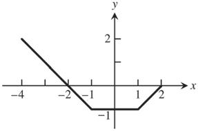
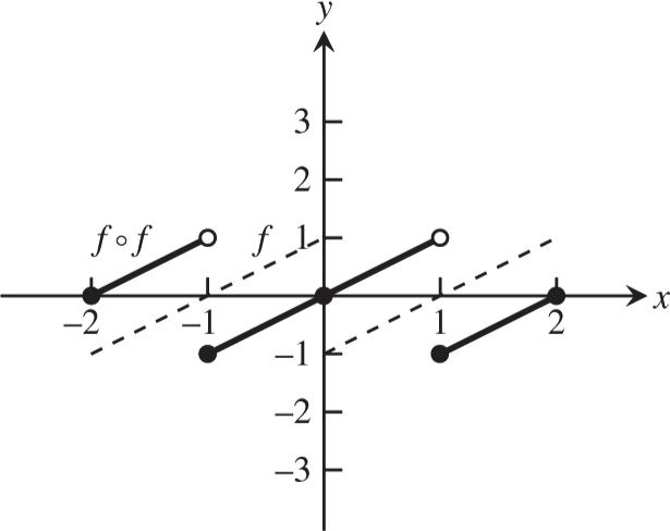
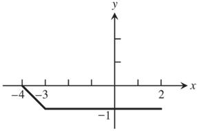
47.
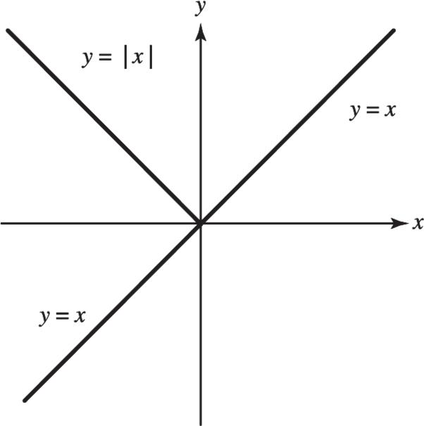
The graph of 21()(||) fxfx is the same as the graph of 1 ()fx to the right of the y-axis. The graph of 2 ()fx to the left of the y-axis is the reflection of 1 (),yfx 0 x across the y-axis.
48.
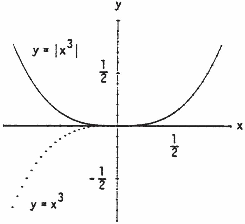
Whenever 1 () g x is positive, the graph of y
2 () g x 1 () g x is the same as the graph of y
1 (). g x When 1 () g x is negative, the graph of y
2 () g x is the reflection of the graph of 1 ()ygx across the x-axis.
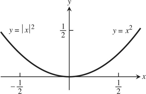
It does not change the graph.
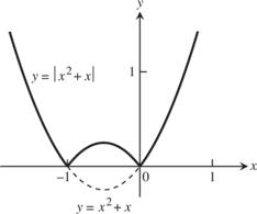
Whenever 1 () g x is positive, the graph of y
2 () g x 1 |()| g x is the same as the graph of y
1 (). g x When 1 () g x is negative, the graph of y
2 () g x is the reflection of the graph of 1 ()ygx across the x-axis.
49.
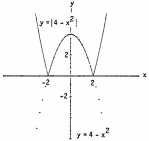
Whenever 1 () g x is positive, the graph of 21()|()|ygxgx is the same as graph of 1 ().ygx When 1 () g x is negative, the graph of 2 ()ygx is the reflection of the graph of 1 ()ygx across the x-axis.
50.
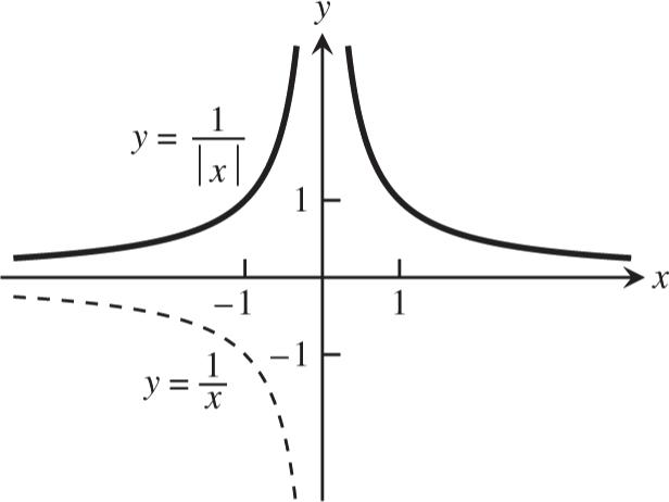
The graph of 21()(||) fxfx is the same as the graph of 1 ()fx to the right of the y-axis. The graph of 2 ()fx to the left of the y-axis is the reflection of 1 (),0yfxx across the y-axis.
Copyright 2023 Pearson Education, Inc.
52.
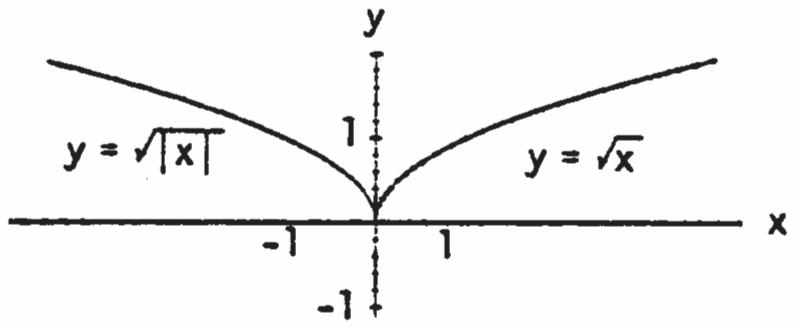
The graph of 21()(||) fxfx is the same as the graph of 1 ()fx to the right of the y-axis. The graph of 2 ()fx to the left of the y-axis is the reflection of 1 (),0yfxx across the y-axis.
53. (a) 1 2 (3)ygx (c) ()ygx (e) 5()ygx
54. (a) Shift the graph of f right 5 units.
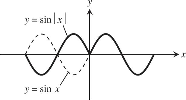
The graph of 21()(||) fxfx is the same as the graph of 1 ()fx to the right of the y-axis. The graph of 2 ()fx to the left of the y-axis is the reflection of 1 (),0yfxx across the y-axis.
(b) 2 3 2 ygx
(d) ()ygx (f ) (5)ygx
(b) Horizontally compress the graph of f by a factor of 4.
(c) Horizontally compress the graph of f by a factor of 3 and then reflect the graph about the y-axis.
(d) Horizontally compress the graph of f by a factor of 2 and then shift the graph left 1 2 unit.
(e) Horizontally stretch the graph of f by a factor of 3 and then shift the graph down 4 units.
(f ) Vertically stretch the graph of f by a factor of 3, then reflect the graph about the x-axis, and finally shift the graph up 1 4 unit.
55. Reflect the graph of y x about the x-axis followed by a horizontal compression by a factor of 1 2 , then shift left 2 units.
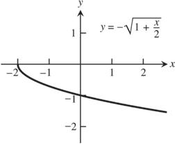
56. Reflect the graph of yx about the x-axis, followed by a vertical compression of the graph by a factor of 3, then shift the graph up 1 unit.
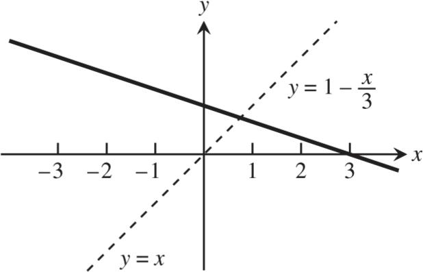
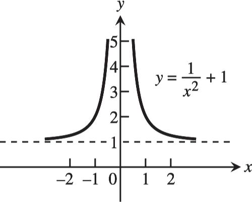
57. Vertical compression of the graph of 2 1 x y by a factor of 2, then shift the graph up 1 unit.
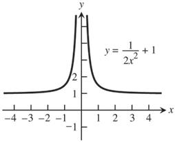
58. Reflect the graph of 1/3 yx about the y-axis, then compress the graph horizontally by a factor of 5.
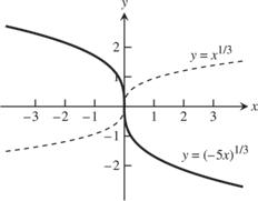
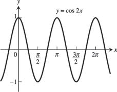
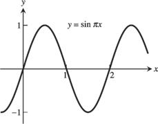
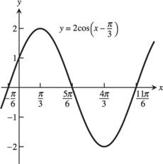
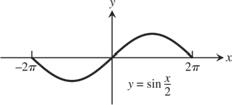
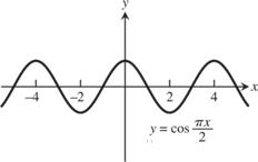
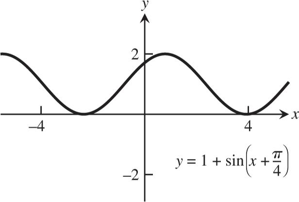
67. (a) tan tan bb BaaB (b) sin sin aa AccA
68. (a) sin a c A (b) 22 sin cb a cc A
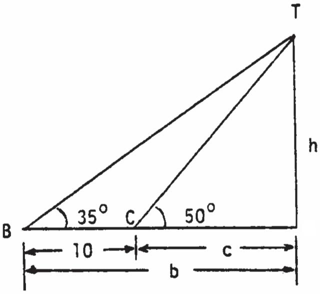
69. Let h height of vertical pole, and let b and c denote the distances of points B and C from the base of the pole, measured along the flat ground, respectively.
Then, tan50 h c , tan35 h b , and 10. bc
Thus, tan50 hc and tan35(10)hbc
tan35 tan50(10)tan35cc (tan50tan35)10tan35 c 10tan35 tan50tan35 tan50 ch c 10tan35tan50 tan50tan35 16.98 m.
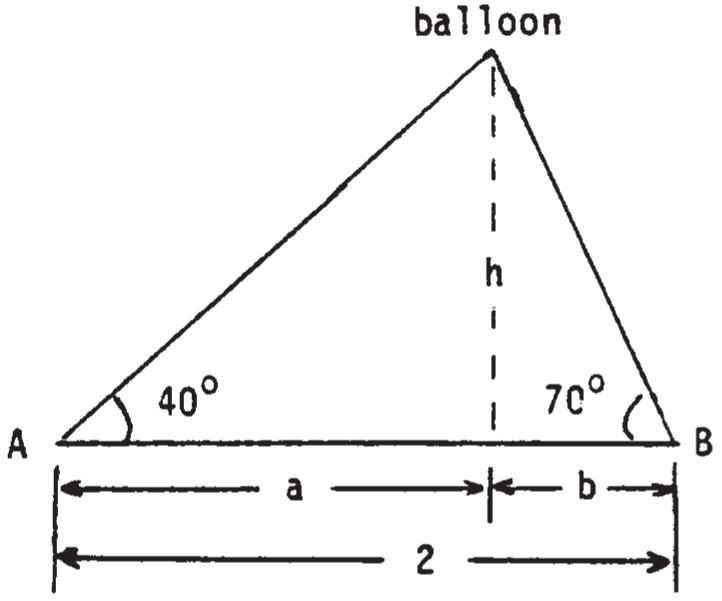
70. Let h height of balloon above ground. From the figure at the right, tan40 h a , tan70 h b , and 2 ab . Thus, tan70(2) hbha tan70 and tan40 ha (2)tan70 a tan40 a (tan40tan70) a 2tan70 a 2tan70 tan40tan70 tan40 ha 2tan70tan40 tan40tan70 1.3 km.
71. (a)
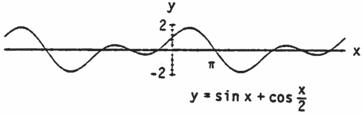
(b) The period appears to be 4. (c) (4)sin(4) fxx 4 2 cos x sin(2) x 22 cos2sincos x x x since the period of sine and cosine is 2. Thus, f (x) has period 4. 72. (a)
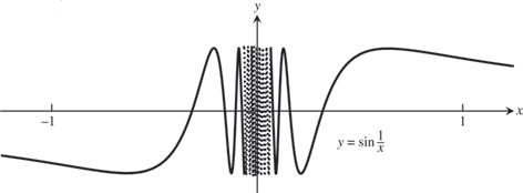
(b) Domain: (,0)(0,); Range: [1,1]
(c) f is not periodic. For suppose f has period p. Then
Choose k so large that 1 2 kp
11 22 sin20 fkpf for all integers k
11 1/(2) 0. kp
But then 1 2 fkp 1 (1/(2)) sin 0 kp which is a contradiction. Thus f has no period, as claimed.
1. There are (infinitely) many such function pairs. For example, ()3 fxx and ()4 g xx satisfy (())(4)3(4)12 fgxfxxx 4(3) x (3)(()). g xgfx
2. Yes, there are many such function pairs. For example, if ()(23)3gxx and 1/3 () fxx , then 3 ()()(())((23)) fgxfgxfx 31/3 ((23))23. xx
3. If f is odd and defined at x, then ()fx ().fx Thus ()()2 gxfx ()2fx whereas ()(()2)gxfx ()2.fx Then g cannot be odd because ()() gxgx ()fx 2 ()fx 2 40, which is a contradiction. Also, () g x is not even unless ()0fx for all x. On the other hand, if f is even, then () g x ()2fx is also even: ()()2 gxfx ()2(). fxgx
4. If g is odd and g(0) is defined, then (0)(0)gg (0). g Therefore, 2(0)0(0)0 gg
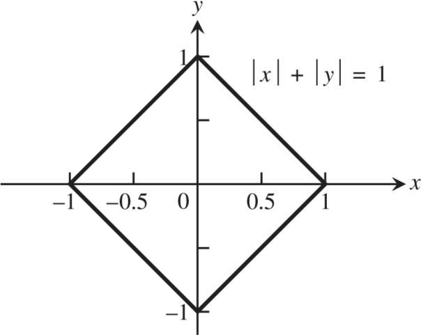
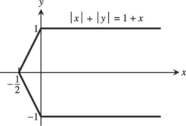
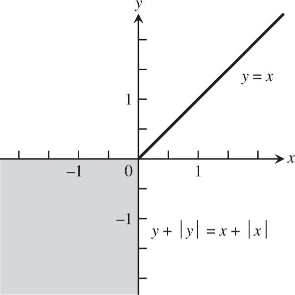
5. For (x, y) in the 1st quadrant, |||| x y 1 x 11 x yxy . For (x, y) in the 2nd quadrant, |||| x y x 1 x y 1 x 21.yx In the 3rd quadrant, ||||1 x yx 1 xyx 21.yx In the 4th quadrant, |||| x y 1()1 x xyx 1. y The graph is given at the right.
6. We use reasoning similar to Exercise 5.
(1) 1st quadrant: |||| yyxx 22. y xyx
(2) 2nd quadrant: |||| yyxx 2()00. yxxy
(3) 3rd quadrant: |||| yyxx ()yy
()00xx all points in the 3rd quadrant satisfy the equation.
(4) 4th quadrant: |||| yyxx ()2 yyx 0. x
Combining these results we have the graph given at the right.
7. (a) 222 sincos1sin x xx 2 1cos x (1cos)(1cos) xx
sin 1cos x x
(b) Using the definition of the tangent function and the double angle formulas, we have
8. The angles labeled in the accompanying figure are equal since both angles subtend arc CD. Similarly, the two angles labeled α are equal since they both subtend arc AB. Thus, triangles AED and BEC are similar which implies 2cos acab bac
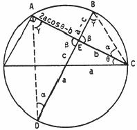
Copyright 2023 Pearson Education,
9. As in the proof of the law of sines of Section 1.3, Exercise 61, sinsin ahbcAabC ac sin B the area of ABC 11 22 (base)(height) ah 111 222sinsinsin bcAabCacB .
10. As in Section 1.3, Exercise 61, 2 (Area of ) ABC 22 1 4 (base)(height) 1122222 44 sin ahabC 222 1 4 (1cos) abC . By the law of cosines, 222 cab 2coscos abCC 222 2 . abc ab Thus, 2222 1 4 (areaof)(1cos)
Therefore, the area of ABC equals ()()() s sasbsc
11. If f is even and odd, then ()() f xfx and ()()()() f xfxfxfx
for all x in the domain of f Thus 2()0()0. fxfx
12. (a) As suggested, let ()() ()(())()() 222 () () () fxfx fxfxfxfx Ex Ex ExE
is an even function. Define ()() 2 ()()()() fxfx OxfxExfx ()() 2 . f xfx Then ()() 2 () f xfx Ox
()()()() 22 () fxfxfxfx OxO is an odd function ()()() f xExOx is the sum of an even and an odd function. (b) Part (a) shows that ()()() f xExOx is the sum of an even and an odd function. If also 11 ()()(), f xExOx where E1 is even and O1 is odd, then ()()0fxfx 11 (()())(()()) ExOxExOx . Thus, ()Ex 11()()() ExOxOx for all x in the domain of f (which is the same as the domain of 1EE and 1OO ). Now 1 ()() EEx ()Ex 1 ()Ex 1 ()() ExEx (since E and E1 are even) ()()11 EExEE is even. Likewise, 11 ()()()() OOxOxOx 1 ()(())OxOx (since O and O1 are odd) 1 (()()) OxOx 1 () OO 1 () x OO is odd. Therefore, 1EE and 1 OO are both even and odd so they must be zero at each x in the domain of f by Exercise 11. That is, 1 EE and 1 ,OO so the decomposition of f found in part (a) is unique.
(a) If 0 a the graph is a parabola that opens upward. Increasing a causes a vertical stretching and a shift of the vertex toward the y-axis and upward. If 0 a the graph is a parabola that opens downward. Decreasing a causes a vertical stretching and a shift of the vertex toward the y-axis and downward.
(b) If 0 a the graph is a parabola that opens upward. If also 0, b then increasing b causes a shift of the graph downward to the left; if 0, b then decreasing b causes a shift of the graph downward and to the right.
If 0 a the graph is a parabola that opens downward. If 0, b increasing b shifts the graph upward to the right. If 0, b decreasing b shifts the graph upward to the left.
(c) Changing c (for fixed a and b) by c shifts the graph upward c units if 0, c and downward c units if 0. c
14. (a) If 0, a the graph rises to the right of the vertical line x b and falls to the left. If <0, a the graph falls to the right of the line x b and rises to the left. If 0 a , the graph reduces to the horizontal line yc As || a increases, the slope at any given point 0 x x increases in magnitude and the graph becomes steeper. As || a decreases, the slope at 0x decreases in magnitude and the graph rises or falls more gradually.
(b) Increasing b shifts the graph to the left; decreasing b shifts it to the right.
(c) Increasing c shifts the graph upward; decreasing c shifts it downward.
15. Each of the triangles pictured has the same base (1sec) bvtv . Moreover, the height of each triangle is the same value h. Thus 1 2 (base)(height) 1 2 bh 123A AA … . In conclusion, the object sweeps out equal areas in each one second interval.
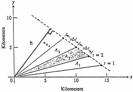
16. (a) Using the midpoint formula, the coordinates of P are
00 2222,,. ab ab Thus the slope of /2 /2 y bb x aa OP (b) The slope of 0 0 b b aa AB The line segments AB and OP are perpendicular when the product of their slopes is
1 bb aa
a Thus, 22 baab (since both are positive). Therefore, AB is perpendicular to OP when .ab
.
17. From the figure we see that 2 0 and 1. ABAD From trigonometry we have the following: sin , EB AB EB cos , AE AB AE tan , CD AD CD and sin cos tan . EB AE We can see that: area AEB area sector DB area 2 11 22 ()()() ADCAEEBAD 1 2 () AD () CD 2 111 222 sincos(1)(1)(tan) sin 111 222cos sincos
18. ()()(())() f gxfgxacxdb and()()(()) acxadbgfxgfx () caxbdacxcbd Thus ()()()() f gxgfxacxadb acxbcdadbbcd Note that () f dadb and (), g bcbd thus ()()()() if ()(). f gxgfxfdgb