Solutions Manual for Managerial Economics and Strategy 4th Edition by Perloff,
Brander
ISBN: 9780135374467
Brander
ISBN: 9780135374467
Demand
1.1 When the price of coffee changes, the change in the quantity demanded reflects a movement along the demand curve. When other variables that affect demand change, the entire demand curve shifts. For example, when income changes, this causes coffee demand to shift.
1.2 Q Y ∂ ∂ = 0.1.
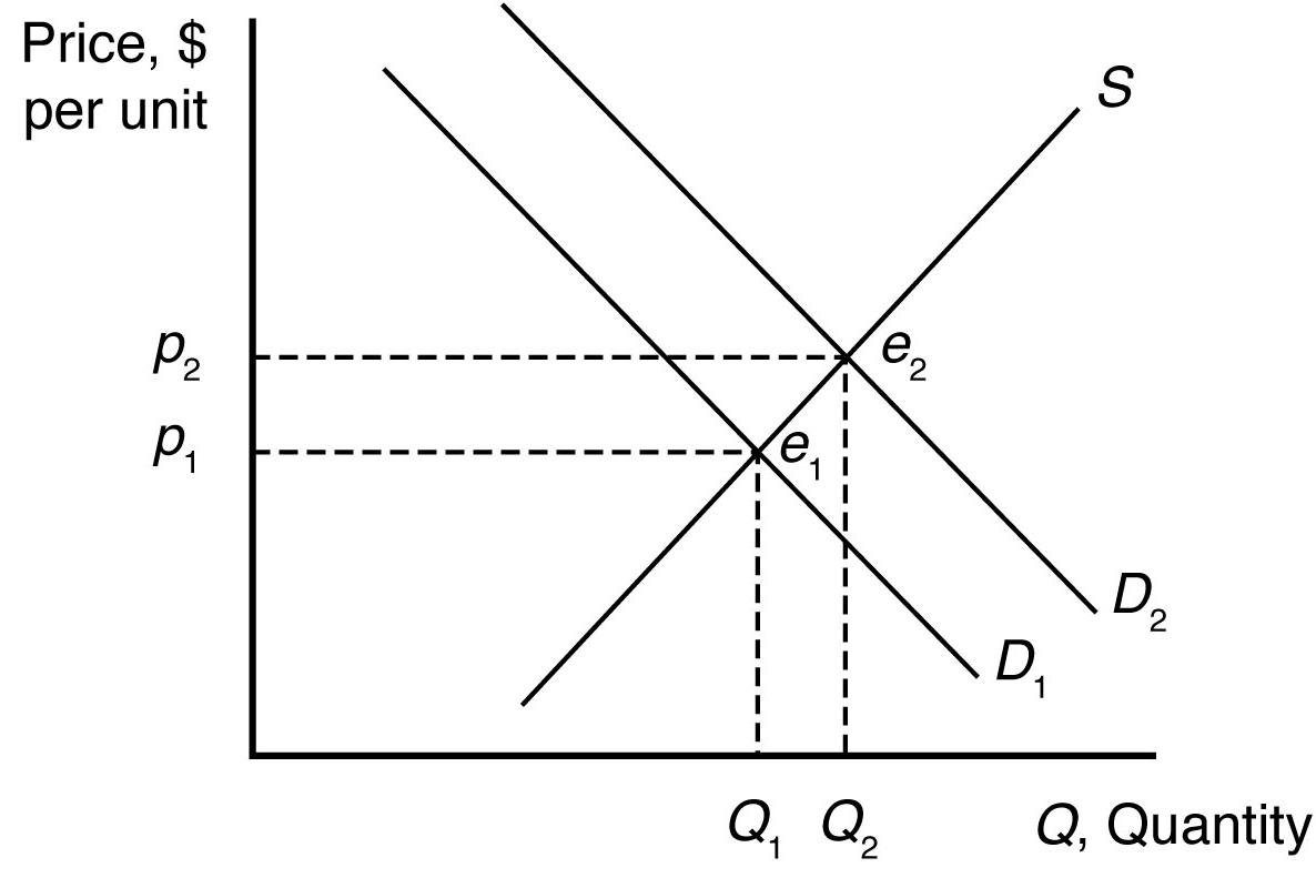
An increase in Y shifts the demand curve to the right, from D1 to D2.
1.3 The relationship between the quantity of coffee (���� ) and the price of sugar (�������� ) is defined by the coefficient on the �������� term in the equation. Since this coefficient is negative (it’s value is 0.3), an increase in the price of sugar (�������� ) will decrease the quantity of coffee. This is the definition of a complementary good. More specifically, if the price of sugar goes up by $1.00 per pound, then the demand for coffee will fall by 300,000 tons.
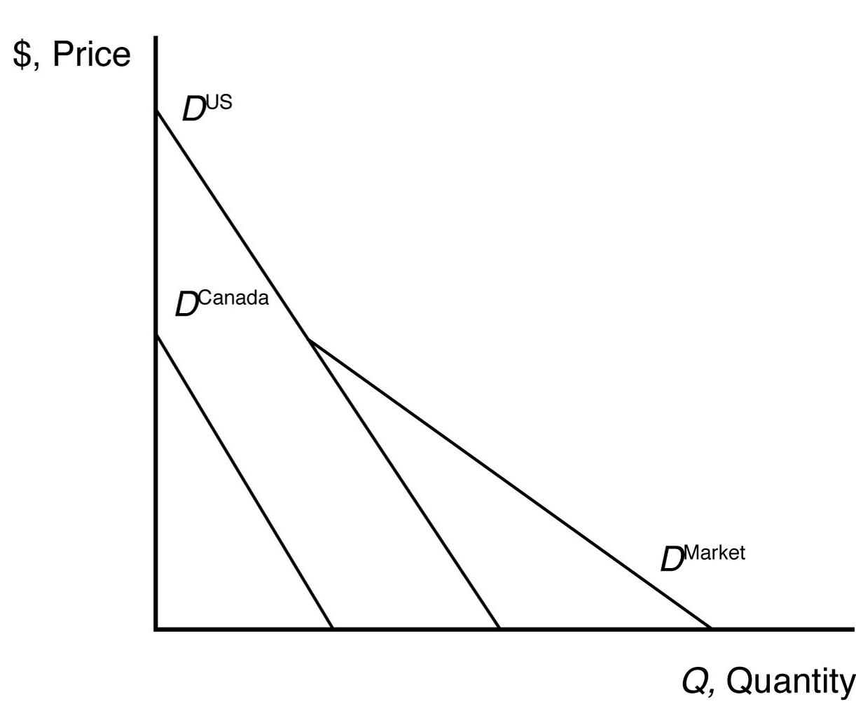
1.4 The market demand curve is the sum of the quantity demanded by individual consumers at a given price. Graphically, the market demand curve is the horizontal sum of individual demand curves.
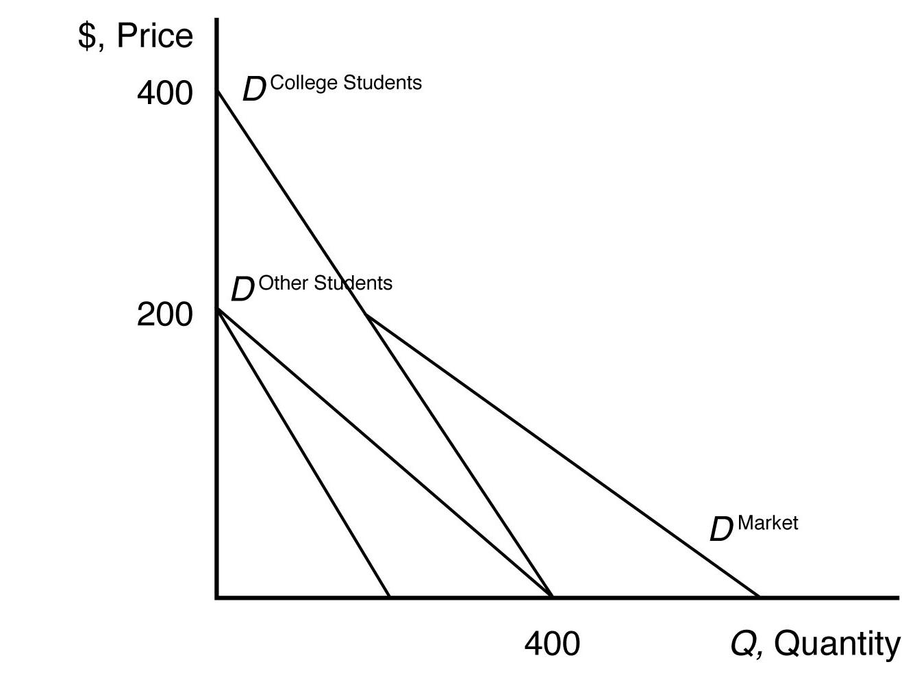
1.5 a. The inverse demand curve for other town residents is p = 200 0.5Qr.
b. At a price of $300, college students demand 100 units of firewood, and other residents demand no firewood. Other residents will demand zero units of firewood if the price is greater than or equal to $200.
c. The market demand curve is the horizontal sum of individual demand curves, as illustrated below.
2.1 The effect of a change in pf on Q is f Q p ∆ ∆ = 20pf f Q p
20(1.10)
22 units.
Thus, an increase in the price of fertilizer will shift the avocado supply curve to the left by 22 units at every price (i.e., a parallel shift to the left).
2.2 When the price of avocados changes, the change in the quantity supplied reflects a movement along the supply curve. When costs or other variables that affect supply change, the entire supply curve shifts. For example, the price of fertilizer represents a key factor of avocado production, which affects the cost of avocado production, shifting the avocado supply curve. This is because avocado prices are measured on a graph axis. Other factors that affect supply are not measured by a graph axis.
2.3 Given the supply function, Q = 58 + 15p–20pf,
The effect of a change in p on Q is
= 15p
To change quantity by 60, price would need to change by 60 = 15p p = $4.00.
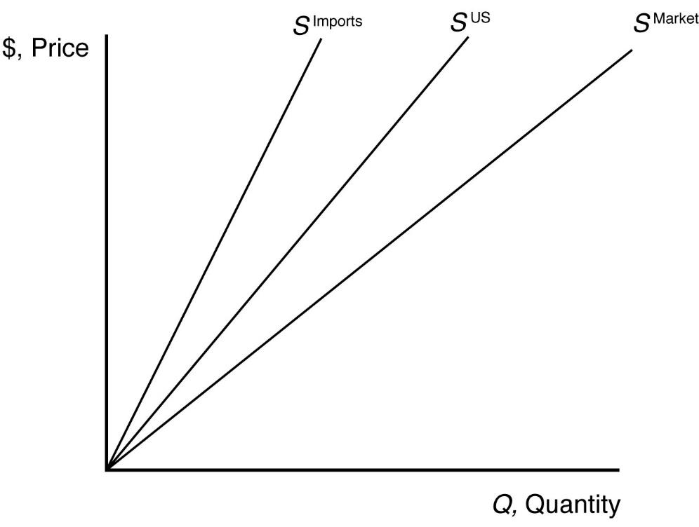
2.4 The market supply curve is the sum of the quantity supplied by individual producers at a given price. Graphically, the market supply curve is the horizontal sum of individual supply curves.
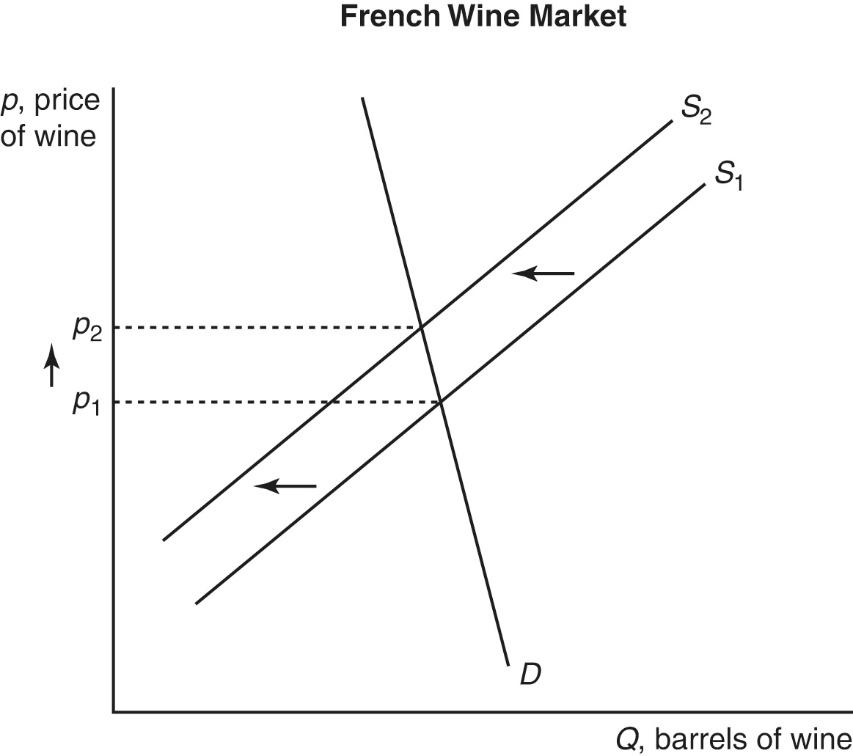
2.5 When the demand curve is steep (as shown in the diagram below), then a shift to the left (inward) of the supply of wine will result in relatively large increases in price and relatively small decreases in quantity. In the diagram, the shift from S1 to S2 drives up price from P1 to P2
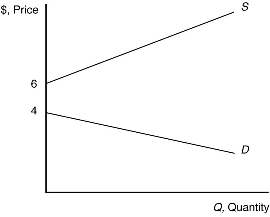
3.1 The supply curve is upward sloping and intersects the vertical price axis at $6. The demand curve is downward sloping and intersects the vertical price axis at $4. When all market participants are able to buy or sell as much as they want, we say that the market is in equilibrium: a situation in which no participant wants to change its behavior. Graphically, a market equilibrium occurs where supply equals demand. An equilibrium does not occur at a positive quantity because supply does not equal demand at any price.
3.2 The equilibrium price is p = $300, and the equilibrium quantity is Q = 2000.
3.3 Given that ps = $0.20, pc = $5, and Y = $55,000 (note Y is measured in thousands, so the value to use here is 55), the demand for coffee can be rewritten as Q = 14 p and the supply of coffee can be rewritten as Q = 8.6 + 0.5p.
When all market participants are able to buy or sell as much as they want, we say that the market is in equilibrium: a situation in which no participant wants to change its behavior. Graphically, a market equilibrium occurs where supply equals demand. Thus, the equilibrium price is
D = S
14 p = 8.6 + 0.5p
5.4 = 1.5p p = $3.60.
Find the equilibrium quantity by substituting this price into either the supply or demand function. For example, using the supply function, the equilibrium quantity is
Q = 8.6 + 0.5p
Q = 8.6 + 0.5(3.60)
Q = 8.6 + 1.8
Q = 10.4 units.
3.4 If Y = $55,000, ps = 0.20, pc = $5, and p = 4, the quantity demanded is Q = 8.56 4 0.3(0.2) + 0.1(55) = 10. The quantity supplied is Q = 9.6 + 0.5(4) 0.2(5) = 10.6. There is an excess supply equal to 10.6 10.0 = 0.6 in this case. Because of the excess supply, firms unable to sell at the price of $4 would lower their prices, forcing the market price down. Price would fall until the equilibrium price was reached.
3.5 The implication is that the price of stocks rose due to excess demand. If this excess demand was caused and a rightward shift of the demand curve, then the complete effect is an increase in the price of stocks along with an increases in the quantity of stocks traded.
4.1
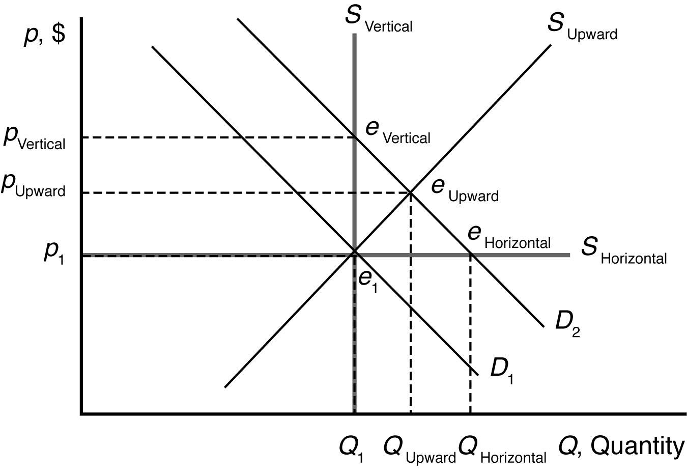
a. The new equilibrium with the horizontal supply curve is where the new demand curve intersects the horizontal supply curve. The new equilibrium price is unchanged. See figure.
b. The new equilibrium with the vertical supply curve is where the new demand curve intersects the vertical supply curve. The new equilibrium price is higher. See figure.
c. The new equilibrium with the upward-sloping supply curve is where the new demand curve intersects the upward-sloping supply curve. The new equilibrium price is higher. See figure.
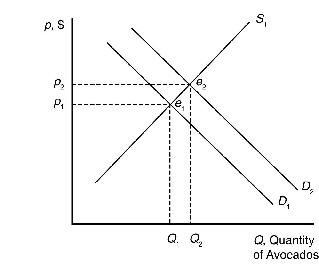
4.2 a. Health benefits from drinking coffee shift the demand curve for coffee to the right because more coffee is now demanded at each price. The new market equilibrium is where the original supply curve intersects the new coffee demand curve, at a higher price and larger quantity.
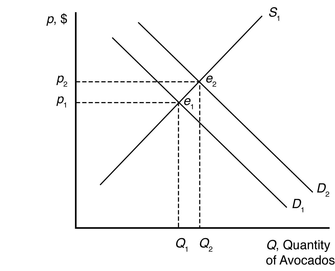
b. An increase in the usefulness of cocoa will increase demand for cocoa. This will drive up the equilibrium price of cocoa. Since cocoa and coffee are likely substitutes, this will increase the demand for coffee. The new market equilibrium is where the original supply curve intersects the new coffee demand curve, at a higher price and higher quantity.
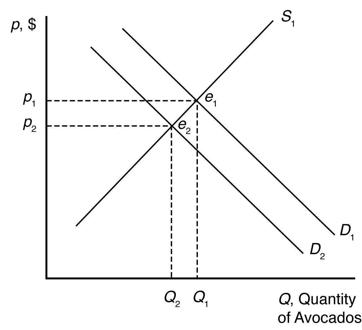
c. A recession shifts the demand curve for coffee to the left because less coffee is now demanded at each price. The new market equilibrium is where the original supply curve intersects the new coffee demand curve, at a lower price and lower quantity.
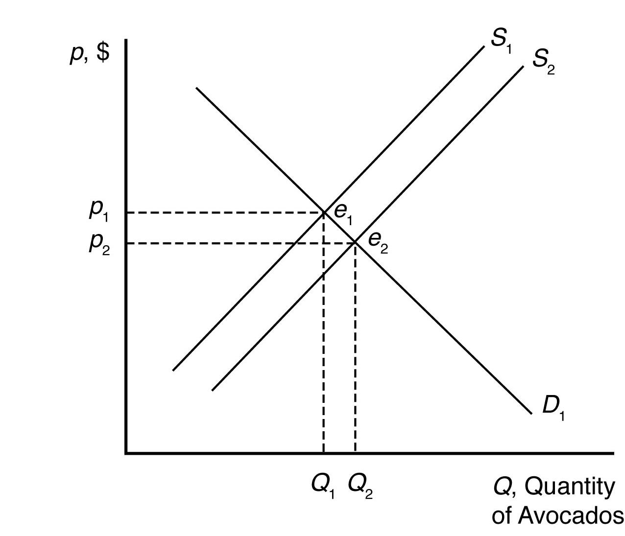
d. New technologies increasing yields shift the supply curve for coffee to the right because more coffee is now supplied at each price. The new market equilibrium is where the original demand curve intersects the new avocado supply curve, at a lower price and higher quantity.
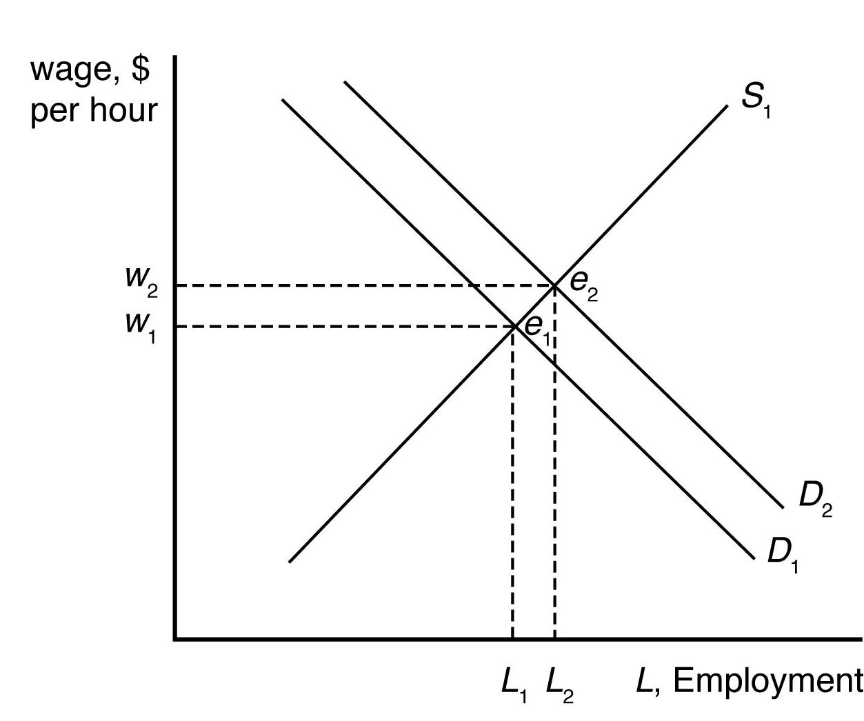
4.3 Outsourcing shifts the labor demand curve to the right because more Indian workers are demanded at each wage. The new market equilibrium is where the original supply curve intersects the new labor demand curve.
4.4 Given that pt = $0.80, the demand for avocados can be rewritten as
Q = 160 40p and the supply of avocados can be rewritten as
Q = 50 + 15p
When all market participants are able to buy or sell as much as they want, we say that the market is in equilibrium: a situation in which no participant wants to change its behavior. Graphically, a market equilibrium occurs where supply equals demand. Thus, the equilibrium price is
D = S
160 40p = 50 + 15p
110 = 55p p = $2.00.
Find the equilibrium quantity by substituting this price into either the supply or demand function. For example, using the supply function, the equilibrium quantity is
Q = 50 + 15p
Q = 50 + 15(2.00)
Q = 50 + 30
Q = 80 units.
When the price of tomatoes increases to $1.35, the demand curve for avocados shifts out to
Q = 171 40p
The supply of avocados is unchanged. The new equilibrium is found where D = S
171 40p = 50 + 15p
121 = 55p
p = $2.20.
The equilibrium quantity is found as before
Q = 50 + 15p
Q = 50 + 15(2.20)
Q = 50 + 33
Q = 83 units.
4.5 A leftward shift in the labor supply curve will drive up wages and reduce employment. The size of these effects will depend on the relative slopes of the supply and demand curves for labor.
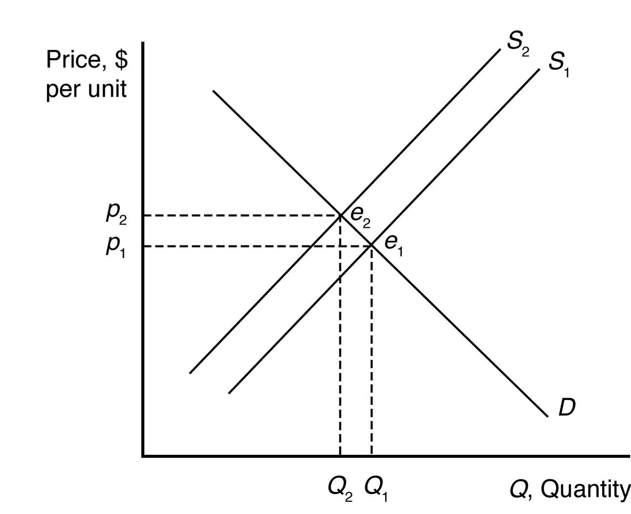
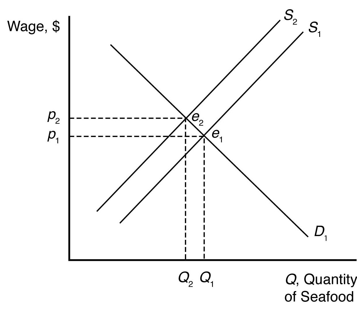
4.6 The damage reduces the supply of oranges, increasing the equilibrium price and decreasing the equilibrium quantity of orange juice.
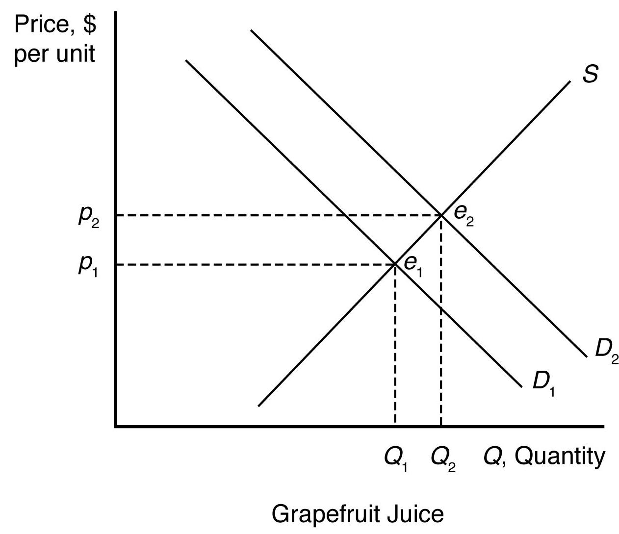
The demand for grapefruit juice increases as the price of orange juice increases because grapefruit juice is a substitute. As the demand for grapefruit juice increases, the equilibrium price and quantity of grapefruit juice increase.
4.7 The increased use of corn for producing ethanol will shift the demand curve for corn to the right. This increases the price of corn overall, reducing the consumption of corn as food.
4.8 Suppose supply is initially S1, but it decreases by a small amount to S2 after the BP oil spill. When all market participants are able to buy or sell as much as they want, we say that the market is in equilibrium: a situation in which no participant wants to change its behavior. Graphically, a market equilibrium occurs where supply equals demand. The original market equilibrium is where the original demand curve intersects the original supply curve (e1). The new market equilibrium is where the original demand curve intersects the new supply curve (e2). When the supply curve shifts by a relatively small amount, the change in the equilibrium price is likely to be small.
4.9 Concerns about botulism caused the demand curve for baby formula to shift in. (A lower quantity was demanded at any given price.) This demand curve shift would put downward pressure on price and quantity. The removal of production permits caused the supply curve to shift in. (A lower quantity was supplied at any given price.) This supply curve shift would put upward pressure on price and downward pressure on quantity. Overall, the price could rise or fall depending on the relative size of the demand curve and supply curve shifts. However, quantity would have to fall.
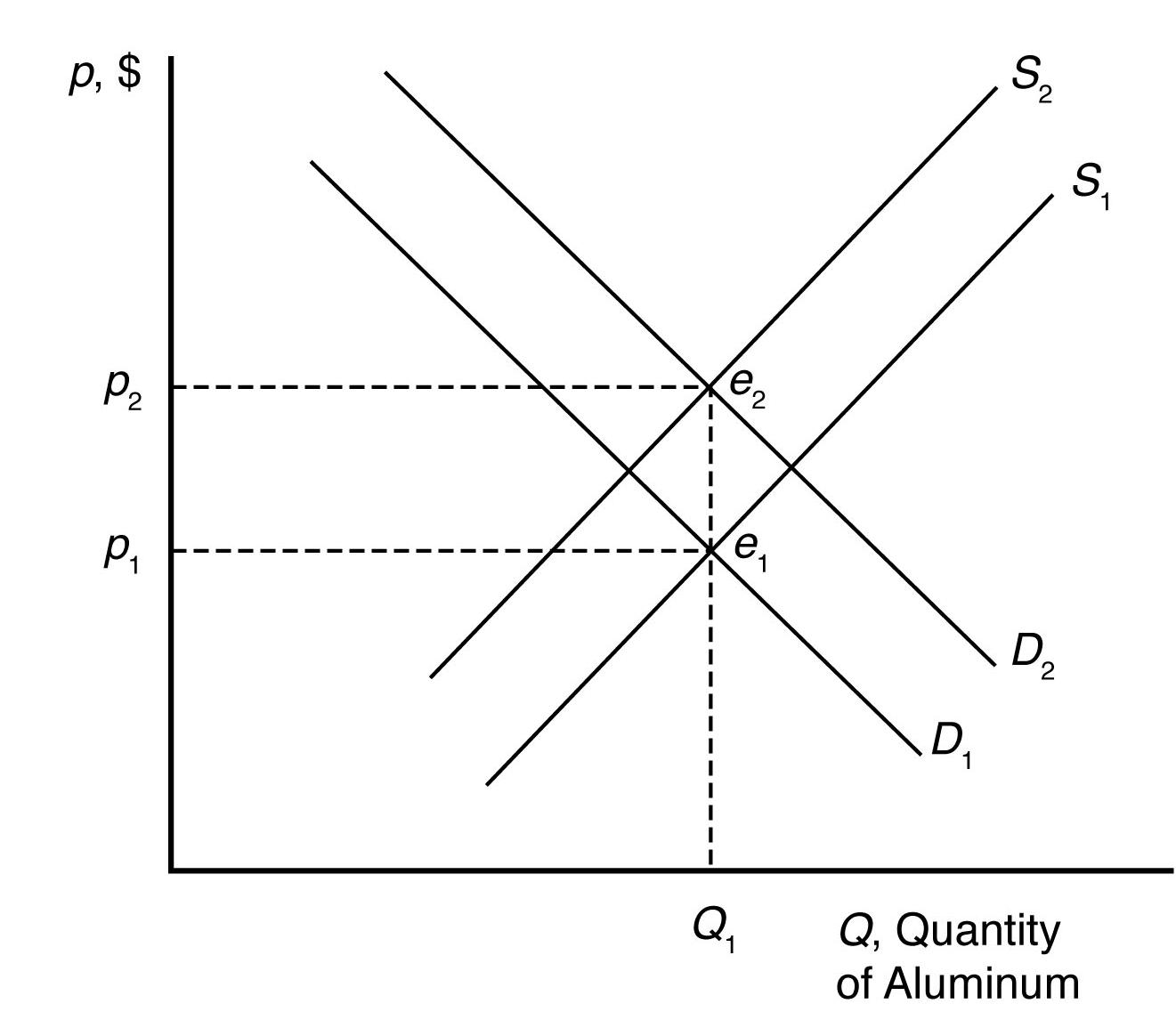
4.10 An increase in petroleum prices shifts the aluminum supply curve to the left because the cost of producing aluminum is more expensive at each price. An increase in the cost of petroleum also shifts the demand curve for aluminum to the right because the petroleum price increase makes a substitute, plastic, more expensive (by making the cost of plastic production higher). The new equilibrium is where the new aluminum supply curve intersects the new aluminum demand curve.
When the supply curve shifts to the left, the new equilibrium price is higher and the new equilibrium quantity is lower. When the demand curve shifts to the right, the new equilibrium price is higher and the new equilibrium quantity is higher. When both curves shift, the new equilibrium price is higher, but the new equilibrium quantity could be higher, lower, or unchanged.
4.11 The cartoon seems to show a bumper harvest of lobsters. A large increase in the catch will shift the supply curve to the right (from S1 to S2) which will cause price to fall from p1 to p2
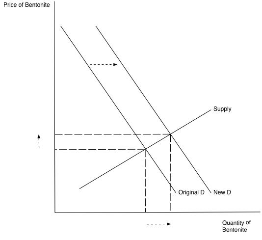
4.12 When drilling increases in response to the rising price of crude oil, the demand for bentonite increases as well. The demand curve will shift to the right and cause the equilibrium price and quantity of bentonite to increase. This is illustrated in the picture below:
5.1 The effect of vendor licensing is to reduce the number of street vendors relative to the undistorted market equilibrium. Therefore, the number of handbags (and other products) offered for sale by street vendors is less than it would be without licensing (with free entry). As a result, the supply curve for handbags available from street vendors has shifted in compared with what it would be without licensing. The diagram representing the street vendor handbag market is therefore similar to the diagram in Q&A 2.2. The market price is higher and the quantity sold is lower than it would be without mandatory licensing.
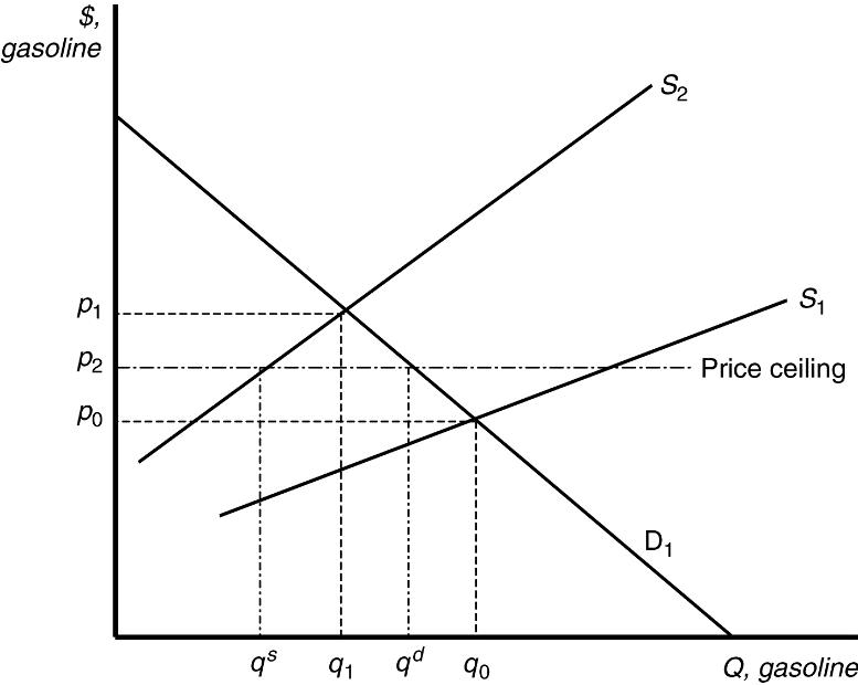
5.2 In the absence of price controls, the leftward shift of the supply curve as a result of Hurricane Katrina would push market prices up from p0 to p1 and reduce quantity from q0 to q1. At a government imposed maximum price of p2, consumers would want to purchase qd units, but producers would only be willing to sell qs units. The resulting shortage would impose search costs on consumers making them worse off. The reduced quantity and price also reduced firms’ profits.
5.3 With a binding price ceiling, such as a ceiling on the rate that can be charged on loans, some consumers who demand loans at the rate ceiling will be unable to obtain them. This is because the demand for bank loans is greater than the supply of bank loans to low-income households with the usury law.
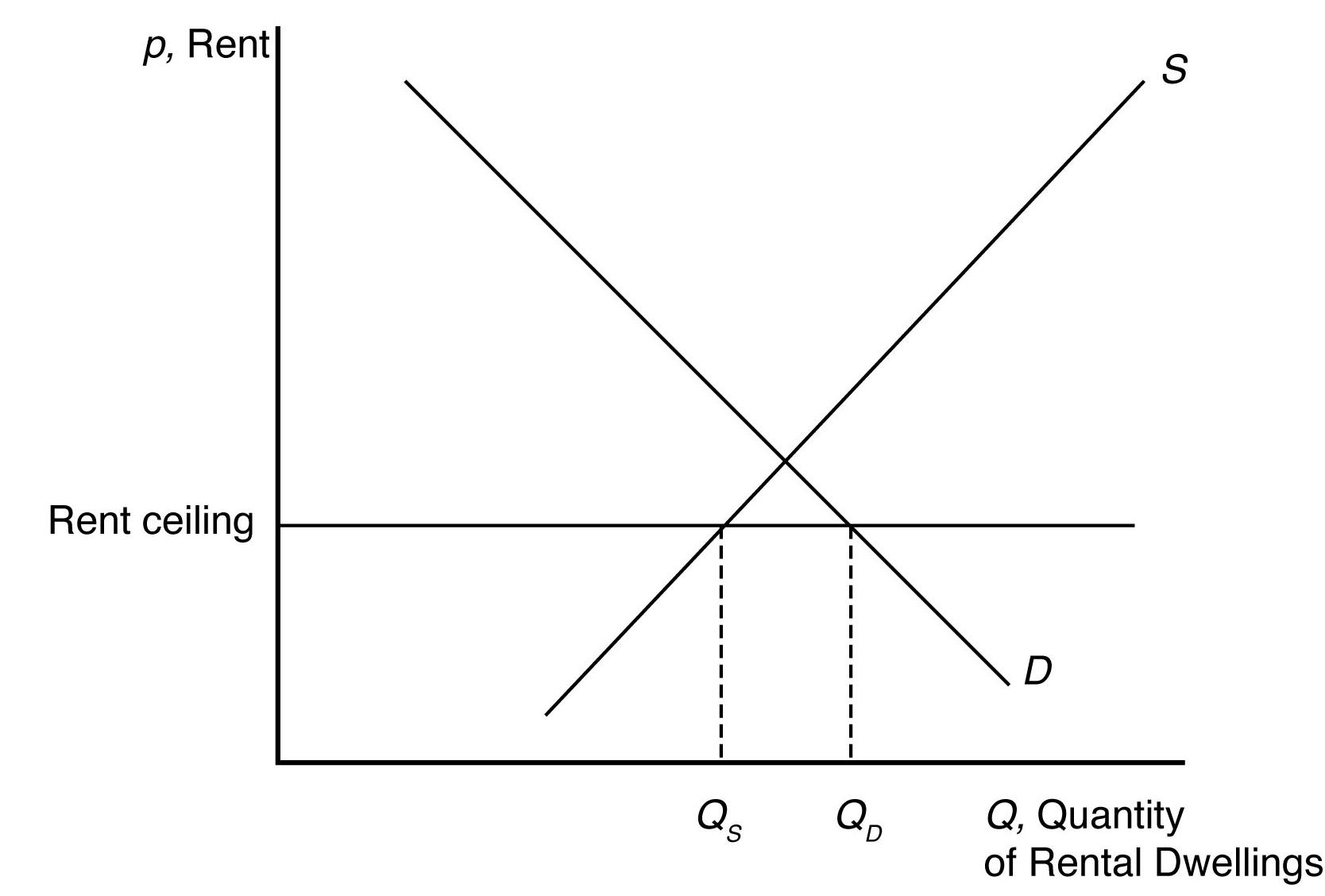
5.4 With the binding rent ceiling, the quantity of rental dwellings demanded is that quantity where the rent ceiling intersects the demand curve (QD). The quantity of rental dwellings supplied is that quantity where the rent ceiling intersects the supply curve (QS). With the rent control laws, the quantity supplied is less than the quantity demanded, so there is a shortage of rental dwellings.
5.5 We can determine how the total wage payment, W = wL(w), varies with respect to w by differentiating. We then use algebra to express this result in terms of an elasticity:
where ε is the elasticity of demand of labor. The sign of d W/dw is the same as that of 1 + ε. Thus, total labor payment decreases as the minimum wage forces up the wage if labor demand is elastic, ε < –1, and increases if labor demand is inelastic, ε > –1.
For a graphical explanation, see the figures below. In the top panel with very flat supply and demand curves, the imposition of a minimum wage causes overall wage payments to fall dramatically. On the other hand, when supply and demand curves are steep (as in the bottom panel), overall wage payments increase substantially.
5.6 Before the tax is imposed, the demand for avocados can be rewritten as Q = 160 40p
and the supply of avocados is given as
Q = 50 + 15p
When all market participants are able to buy or sell as much as they want, we say that the market is in equilibrium: a situation in which no participant wants to change its behavior. Graphically, a market equilibrium occurs where supply equals demand. Thus, the equilibrium price is
D = S
160 40p = 50 + 15p
110 = 55p
p = $2.00.
Find the equilibrium quantity by substituting this price into either the supply or demand function. For example, using the supply function, the equilibrium quantity is
Q = 50 + 15p
Q = 50 + 15(2.0)
Q = 50 + 30
Q = 80 units.
If a $0.55 tax is imposed, the demand curve can be rewritten to account for the tax. First, the demand curve can be rewritten as inverse demand by solving for p
Q = 160 40p
p = 4 0.025Q.
The tax is subtracted from inverse demand to give p = 3.45 0.025Q and then this inverse demand curve can be turned back into a demand curve
Q = 138 40p.
Setting supply equal to demand, the new equilibrium (pretax) price is
D = S
138 40p = 50 + 15p 88 = 55p p = $1.60.
The after-tax price is $2.15.
Using the supply function, the equilibrium quantity is
Q = 50 + 15p
Q = 50 + 15(1.60)
Q = 50 + 24 Q = 74 units.
5.7 a. If demand is vertical and supply is upward sloping, then all the tax burden is paid by consumers because they are not price sensitive.
b. If demand is horizontal and supply is upward sloping, then all the tax burden is paid by producers because consumers are infinitely price sensitive.
c. If demand is downward sloping and supply is horizontal, then all the tax burden is paid by consumers because producers are infinitely price sensitive.
5.8 If instead of the tax being levied on producers it is collected from consumers, then the effect will be a decrease in demand. The demand curve will shift left until the vertical distance between the original demand curve and the new one is equal to the tax of $2.40. This new demand curve, call it D2, will intersect the original supply curve (S1) at a price of $5.60 and a quantity of 11.6. In addition to the price of $5.60 per bushel, buyers will also have to pay the $2.40 tax for a total, after-tax price of $8.00. The seller will receive the $5.60 per bushel, and the government will collect $27.84 billion in tax revenue (the $2.40 tax multiplied by the 11.6 billion bushels of corn traded in the new equilibrium).
This equilibrium is not the same as the case in Q&A 2.3 because in that problem the supply curve is perfectly elastic, while in this case it is not. In Q&A 2.3, the seller passes on the entire tax to consumers, while here, the tax is split with $0.80 being paid by consumers and $1.60 paid by producers.
5.9 A tax on consumers will undoubtedly shift the demand curve down by an amount equal to the size of the tax. The new equilibrium price and quantity with the tax will be where the new demand curve intersects the original supply curve. The decrease in quantity will be larger (and tax revenue smaller) the more horizontal the supply curve is. Just the opposite is true if the supply curve is more vertical quantity effects will be small, and revenue generation from the tax will be large.
6.1 The supply-and-demand model is accurate in perfectly competitive markets, which are markets in which all firms and consumers are price takers: no market participant can affect the market price. If there is only one seller of a good or service a monopoly that seller is a price taker and can affect the market price. Firms are also price setters in an oligopoly a market with only a small number of firms. Experience has shown that the supply-and-demand model is reliable in a wide range of markets, such as those for agriculture, financial products, labor, construction, many services, real estate, wholesale trade, and retail trade.
7.1 A tax paid by consumers shifts the demand curve down by an amount equal to the size of the tax. Just the opposite, suspending a tax on consumers should raise the demand curve by an amount equal to the size of the suspended tax. Although fuel supply is more likely to be vertical in the short run than in the long run, equilibrium fuel prices will increase when the demand curve shifts up whether the supply curve is vertical or upward sloping.
Solutions Available on MyLab Economics
CHAPTER OUTLINE
Managerial Problem: Carbon Taxes
2.1 Demand
The Demand Curve
Effects of a Price Change on the Quantity Demanded Effects of Other Factors on Demand
The Demand Function
Using Calculus: Deriving the Slope of a Demand Curve
Summing Demand Curves
Mini-Case: Summing Corn Demand Curves
2.2 Supply
The Supply Curve
Effects of Price on Supply
Effects of Other Variables on Supply
The Supply Function
Summing Supply Curves
2.3 Market Equilibrium
Using a Graph to Determine the Equilibrium
Using Math to Determine the Equilibrium
Forces That Drive the Market to Equilibrium
Mini-Case: Speed of Adjustment to New Information
2.4 Shocks to the Equilibrium
Effects of a Shift in the Demand Curve
Q&A 2.1
Effects of a Shift in the Supply Curve
Mini-Case: The Opioid Epidemic Reduces Labor Market Participation
Q&A 2.2
Managerial Implication: Taking Advantage of Future Shocks
2.5 Effects of Government Interventions
Policies That Shift Curves
Mini-Case: Occupational Licensing
Price Controls
Price Ceilings
Mini-Case: Venezuelan Price Ceilings and Shortages
Why Supply Need Not Equal Demand
Sales Taxes
Equilibrium Effects of a Specific Tax
Equilibrium Is the Same No Matter Whom the Government Taxes
Pass-Through
Q&A 2.3
Managerial Implication: Cost Pass-Through Mini-Case: Taxes on Fattening Foods
2.6 When to Use the Supply-and-Demand Model
Managerial Solution: Carbon Taxes
Summary
Questions
1. Demand: The quantity of a good or service that consumers demand depends on price and other factors such as consumer incomes and the prices of related goods.
2. Supply: The quantity of a good or service that firms supply depends on price and other factors such as the cost of inputs and the level of technological sophistication used in production.
3. Market Equilibrium: The interaction between consumers’ demand and producers’ supply determines the market price and quantity of a good or service that is bought and sold.
4. Shocks to the Equilibrium: Changes in a factor that affects demand (such as consumer income) or supply (such as the price of inputs) alter the market price and quantity sold of a good or service.
5. Effects of Government Interventions: Government policy may also affect the equilibrium by shifting the demand curve or the supply curve, restricting price or quantity, or using taxes to create a gap between the price consumers pay and the price firms receive.
6. When to Use the Supply-and-Demand Model: The supply-and-demand model applies very well to highly competitive markets, which are typically markets with many buyers and sellers.
This is obviously an important chapter and while much of this material will be review for many students, a good, solid understanding of the basics here will pay big dividends later.
Demand: This is a good place to begin since most students have experience thinking about market situations from the perspective of a consumer. Whether students have been exposed to this material previously or not, one of the trickiest parts in this section is the distinction between a change in price and a change in any of the other determinants of demand. The former, of course, leads to a change in quantity demanded and a movement along the demand curve, while the latter leads to a change in demand and a shift of the entire demand curve. It is helpful to point out that this distinction is somewhat artificial and is driven by the fact that the demand relationship is being represented graphically in two dimensions. Depending on the mathematical preparation of the class, it can be very helpful to discuss the demand relationship algebraically without worrying about drawing the diagram. This allows for multiple right-hand side variables in the demand function and no concern about which one leads to which type of change. For some students, this can be an eyeopening observation.
Supply: The discussion here parallels the discussion in the section on demand. The biggest difference is that students are not as familiar with taking the perspective of a producer, and so additional discussion might be necessary to get them thinking in this way. The same technical concern arises with a shift in the supply curve versus a movement along the curve, but it can be handled the same way that it was in discussing demand.
Market Equilibrium: If there is one result that students are likely to recall from past coursework, it is the fact that the intersection of the supply and demand curves marks the equilibrium point in the market. Despite this familiarity, however, it is important to take the time to work through any parts of the discussion that are new (e g., solving for equilibrium price and quantity algebraically).
It is often easier to remind students of why the intersection of supply and demand is the equilibrium by considering prices that are both higher and lower. Label the (potential) equilibrium price in the diagram and then ask students to think about high prices (those above this proposed value) and low prices (those below this value). It should be relatively easy for students to recall and see that at high prices there is a surplus where quantity supplied exceeds quantity demanded. It also should be relatively easy for them to suggest that prices should fall in this circumstance. Likewise, at low prices there will be a shortage as quantity demanded exceeds quantity supplied. This disequilibrium should lead to rising prices. This leaves only the point where quantity supplied equals quantity demanded as the spot where there is no market pressure for prices to rise or fall, i.e., the market is in equilibrium.
Shocks to the Equilibrium: This is the basic story of comparative statics. Students probably will be familiar with this type of analysis from a graphical, qualitative perspective, but it is a good idea to spend some time showing them how the same analysis can become more quantitative in the presence of specific functional forms for supply and demand. This is an opportunity to practice some basic algebra skills and also serves as motivation for the estimation of demand and supply functions that will be coming up in Chapter 3.
Effects of Government Interventions: There are two topics here: price ceilings and floors and sales taxes. The discussion on price ceilings and floors should be pretty straightforward after discussing equilibrium and why prices above and below market equilibrium are not balanced. An effective price ceiling or floor essentially creates a persistent disequilibrium with a resulting excess shortage or surplus. Care should be taken to emphasize that not all price ceilings and floors result in disequilibrium and that it is important to compare the price restriction to the actual market equilibrium to determine whether there will be any effect.
The discussion on sales taxes is less intuitive and often takes work for students to understand. The key result is that the effect of tax is determined solely by the nature of supply and demand and not by the administrative decision about who should remit the tax to the taxing authority. Perhaps the most effective way to make this point (and it provides good practice as well) is to work through a numerical example. It also can be helpful for students to work out and discuss the results of taxes imposed in markets with extreme supply and demand relationships (vertical or horizontal supply and/or demand curves).
When to Use the Supply-and-Demand Model: This short section makes the important point that not all market situations are suitable for analysis with the supply-and-demand model. Taking a few minutes to point out that this model is a description of a competitive market will help students avoid the common mistake of misapplying these results later on.
Is This Economics or Chemistry? One of my favorite examples to use when teaching about equilibrium and comparative statics in the supply and demand model involves a trip down memory lane. I tell students the story of my first chemistry lab as a young lad in high school. What was so interesting about this lab experience, and the way it relates to teaching about equilibrium, is that the exercise involved a period of great disequilibrium. In the chemistry experiment, this disequilibrium took the form of a bubbling, stinky liquid. The experiment started with all the chemicals in equilibrium – a beaker with a clear liquid, a test tube with a gray powder, etc. The task for the lab was to mix them together and, based on the changes that occurred, determine the identity of each of the original components. So, initial equilibrium was followed by bubbling and stink which, in turn, was followed by a new equilibrium. We then compared the starting point to the ending point essentially doing comparative statics in chemistry lab.
A Classroom Experiment This topic more than any other in the course lends itself to a demonstration in the form of a classroom experiment. There are many different ways to give students the experience of seeing an equilibrium price and quantity develop, but one of my favorites is one from Charlie Holt (Holt, Charles A. “Classroom Games: Trading in a Pit Market,” Journal of Economic Perspectives, 10:1 (Winter 1996), 193-203). The beauty of an exercise like this is that it gives students the opportunity to really feel market forces at work. You can spice up the experiment by bringing along some prizes (candy bars work well) to get everyone motivated to play seriously.
1. Explain why the difference between a shift in the demand curve and movement along the demand curve is so important. Explain why it becomes less important once we leave two-dimensional diagrams behind.
2. Can you think of examples of taxes that are largely paid for by consumers? What about those that are likely to be paid for by producers? Explain why who pays is different from who is responsible for sending the tax money off to the taxing authority.
3. Give an example of a market that is likely to be similar to the supply and demand model presented here. How about one that is very different?
4. What are the sales and income tax rates in your state? What would happen if these taxes were reduced and a carbon tax took their place? Do you think this is a good idea?
5. What is a “sin” tax (see Mini-Case: Taxes on Fattening Foods)? What goods, if any, do you think the government should tax to encourage healthy habits?