
Advanced Science Research Journal


ADVANCED SCIENCE RESEARCH PROGRAM
The Breck Advanced Science Research Program is the capstone course of the Breck science curriculum. This program gives students who are passionate about science and engineering the opportunity for an authentic, high-level summer research experience in collaboration with research professionals in universities, colleges or businesses.
Following the summer research component of the program, students participate in a year-long science research seminar class where they write and submit formal research papers and project presentations to the Twin Cities Regional Science Fair, Regional Junior Sciences and Humanities Symposium and the Minnesota State Science and Engineering Fair, with some students continuing on to the National Junior Sciences and Humanities Symposium or the International Science and Engineering Fair. In addition, Advanced Science Research students participate in a formal seminar at Breck where they present their work to family members, research advisors, and peers.
More information about the Breck School Advanced Science Research Program is available on our website: breckschool.org/asr.
Dr. Kati Kragtorp, Director Advanced Science Research Program
Cover artwork created by Victor Chapple ’25
TABLE OF CONTENTS
Pulling the Pressure Piece
Defining the Role of Piezo1 in a Mouse Model With Rheumatoid Arthritis
Graham Bailey and Samantha Dvorak
Turf Trouble
Does the DEET in bug repellent really kill grass? Year II
Abigail Endres and Selena Qiao
Immune Interference
Is aberrant DUX4 expression responsible for the downregulation of MHC class I genes stimulated by IFN-γ?
Abigail Getnick and Kelan McKay.
Farewell Forever
Degradation of Pentadecafluorooctanoic Acid Using UV-C Light and Titanium Dioxide
Dawson Miller and Caleb Li
The Piece Within Using Matrix Metalloproteinases to Cleave CD200 to Combat Cancer
Structure
Does Caffeine Help You Study? Investigating the effects of caffeine on adolescents’ long-term memory and sustained attention
Health Evaluation Robot for Basil – HERB
A modular robotic system for detecting nutrient deficiency in greenhouse basil
Unique Creeks
Monitoring Nutrient and Bacteria Levels in Rivers to Determine Factors Affecting Water Quality
Charlo Vasicek
Use your mobile phone to scan the QR code included in each article to watch videos of our students’ presentations.
Pulling the Pressure Piece:
Defining the Role of Piezo1 in a Mouse Model With Rheumatoid Arthritis
Graham Bailey and Samantha Dvorak
Introduction
Autoimmune diseases affect 10% of the world’s population (Autoimmune Disorders Found to Affect Around One in Ten People | University of Oxford, 2023). Affected patients experience chronic and painful symptoms that reduce their quality of life Despite the wide impact of autoimmune diseases, the various pathways behind them are not fully understood, leaving patients with limited access to adequate treatments. Two such autoimmune diseases, rheumatoid arthritis (RA) and autoimmune valvular carditis affect millions of people around the world In the case of RA, up to 1% of the world’s population is affected, and, although valvular carditis is rare within the United States, it affects 40 million people around the world and is more common in areas with limited access to antibiotics (Osinski et al , 2024)
To fight off infections, the immune system has a complex organization of cells that are capable of recognizing and killing foreign invaders This requires molecular recognition of antigens so a coordinated response can be mounted To prevent the immune system from accidentally attacking the body, there are complex mechanisms that allow it to recognize material in the body as “self” and prevent the development of an autoimmune disease Several factors cause tolerance mechanisms to break down, including similar molecular structures between foreign antigens and other materials present in the body When tolerance mechanisms fail, the patient develops an autoimmune disease (Autoimmune Disease - an Overview | Science Direct Topics, n.d.). Despite similarities in the overall mechanism, there are a vast number of different autoimmune diseases, and a lot of diversity even within a single disease Because of this, treating autoimmune diseases frequently

focuses on dampening the entire immune system rather than targeted treatment, putting patients at risk for serious infections
In one type of autoimmune infection, rheumatic fever, a build-up of autoantibodies due to Group A Streptococcus infection causes an immune attack on various tissues throughout the body When antibiotic access is limited, patients can experience prolonged and repetitive infections (Marijon et al., 2012). The molecular similarities between Streptococcus antigens and human proteins, including cardiac myosin and extracellular matrix protein laminin, can cause molecular mimicry in which the immune system mistakes a self-component for a foreign antigen (Galvin et al., 2000). Activated B cells produce antibodies against the peptide, causing a build-up of autoantibodies that circulate through the body People with these autoantibodies will sometimes subsequently develop rheumatic fever, in which the heart and joints become temporarily inflamed (Galvin et al., 2000). Repeated exposures to Streptococcus antigens, and subsequent repeated episodes of rheumatic fever, increase the chance of developing long-term autoimmune diseases, such as RA and autoimmune valvular carditis.
In RA, disease progression begins with an immune response towards the joints in the body. As neutrophils are recruited into the joint cavity, they secrete leukotrienes, including leukotriene B4 (LTB4), which stimulates the mass infiltration of neutrophils (Chen et al., 2006). After leukocytes have invaded the synovial membrane, surrounding fibroblasts and macrophages are also activated, causing cartilage destruction and bone erosion (Smolen et al , 2018) As the disease progresses, patients begin to develop hyperplasia, resulting in tissue growth that fully surrounds the joint, known as a
Graham Bailey and Samantha Dvorak
synovial pannus, that causes additional damage to the bone and cartilage in the joint (Chen et al., 2006) This process causes long-term joint damage, decreased mobility, and chronic pain characteristic of RA (Smolen et al , 2018)
Through a similar and sometimes concurrent disease mechanism, autoimmune-induced valvular carditis causes chronic inflammation of the mitral valve, leading to calcification, stenosis, and oftentimes congestive heart failure (Marijon et al , 2012) In valvular carditis, autoantibodies bind to the mitral valve, causing inflammation and infiltration of immune cells, fibrosis, and extracellular matrix growth (Raizada et al , 1983) As valvular carditis progresses, the mitral valve thickens and calcifies, preventing normal function and allowing blood to leak between the chambers of the heart (Marijon et al., 2012). Eventually, the mitral valve’s reduced functionality requires a valve transplant; however, many patients with this disease have limited access to healthcare, and are unable to receive one Even when patients are able to get a transplant, only the symptoms of the disease are being treated, and not the underlying mechanisms that caused it, putting them at risk for further complications (Marijon et al , 2012)
The K/B.g7 mouse model is used to replicate and research Rheumatic Heart Disease (RHD) and RA disease progression. Though these mice develop autoantibodies against a different antigen than in humans with RHD and RA, the cellular mechanisms resulting from these autoantibodies are comparable. The K/B.g7 mouse model has a transgenic T cell receptor (TCR), called KRN, and additionally expresses the Major Histocompatibility Complex (MHC) Class II molecule g7 a combination that induces arthritis and valvular carditis in mice (Monach et al., 2007). K/B.g7 mice produce anti-glucose-6-phosphate isomerase (GPI) autoantibodies that cause the immune system to attack the joints and mitral valve (Monach et al , 2007) Autoreactive T cells then recruit B cells that produce anti-GPI autoantibodies, which accumulate in the joints and are assumed to
accumulate along the lining of the mitral valve (Breed & Binstadt, 2015). This antibody deposition targets the tissues of the joints and heart valve for attack by the immune system In the K/B g7 mouse line, the mitral valve is infiltrated by macrophages and CD4+ KRN T cells (Gorton et al., 2010). A transfer of serum from K/B.g7 mice to a non-K/B.g7 mouse induces autoimmune- mediated arthritis that is less severe than arthritis in K/B g7 mice, and does not induce valvular carditis
In patients with RA and RHD, the tissues surrounding areas affected by inflammation experience greater mechanical stress (Liu et al., 2022) In RA, synovitis causes increased joint stiffness, and in RHD, blood flow causes high mechanical pressure Mechanosensing proteins and ion channels are capable of sensing and responding to the stress present in the joint and heart (Liu et al , 2022) PIEZO1 is a mechanically sensitive ion channel capable of responding to mechanical stress by promoting inflammation (Liu et al , 2022) Based on the known proinflammatory effect of PIEZO1 in other heart diseases and its involvement in immune responses in the heart valves and joints of K/B g7 mice, it is theorized that PIEZO1 promotes the chronic inflammation observed in autoimmune valvular carditis and arthritis (Xie et al., 2023).
To study the effect of PIEZO1 on RA, we compared data on the severity of inflammation, bone erosion, and cartilage erosion in ankle tissue from Tcsf21-Cre Piezo1 floxed mice (Piezo-) to that of wild-type/Tcsf21-Cre mice (Piezo+). The Piezo- mice have Piezo1 deleted from Tcsf21-expressing fibroblasts, which was theorized to promote inflammation in this model and may be similar in humans We also analyzed the morphology of hematoxylin and eosin (H&E) stained heart sections to make sure this remained unaffected in the Piezo- model.
Materials and Methods
Mice treatment and tissue collection
Piezo1 fl/fl Tcf21Cre+ (Piezo-) and wt/fl Tcf21Cre+ (Piezo+) mice were treated, handled,
assessed, and sacrificed by trained researchers, according to an established, IACUC-approved protocol, as part of the ongoing research conducted by this lab We did not have any direct interaction with the mice Serum from K/B.g7 mice was injected into recipient Piezoand Piezo+ mice. The recipient mice received two doses of 150 μL of serum given two days apart, totaling to 300 μL These mice were sacrificed on day 11 After the mice were sacrificed, their ankles and hearts were fixed in paraformaldehyde. Other researchers sectioned and stained the ankle sections using H&E, TRAP, and Safranin O.
Fixed mouse heart embedding protocol
Paraformaldehyde-fixed hearts in 30% sucrose solution stored at -20°C were put in a paper towel. A razor blade was used to cut off the apex of the heart about 1mm up from the tip. Then, while squeezing with tweezers to avoid air bubbles in the heart chambers, the heart was put in a 15 mm cube base mold filled with Optimal Cutting Temperature Compound (OTC Compound; Tissue Tek). The base mold was frozen using -20°C isopentane with dry ice then stored at -80°C.
Cryosectioning of heart tissue for mitral valve protocol
OTC molds with hearts were cryosectioned in a LEICA CM3050 S cryostat at -22°C Molds were mounted using OTC Compound then trimmed in 30 µm sections, adjusting the orientation until the blade was at the same angle as the heart. Additional sections were removed until two separate chambers of the heart appeared, after which the width of sections was shortened to 8 µm Once the mitral valve was reached, the next 45 to 30 sections were plac ed three to a slide on positively charged slides.
Cryosectioning of heart tissue for mitral valve protocol
Slides with the desired tissue were submerged in a 1x PBS (Gen Clone) for 5 minutes The area around the sections were dried, then outlined
Graham Bailey and Samantha Dvorak
with a pap pen (Invitrogen Super Pap Pen 00-8899).
Hematoxylin and Eosin Staining of frozen heart and ankle sections protocol
Sections were covered with hematoxylin quick stain (Vector lab; H-3404) and allowed to sit for two minutes Then, the hematoxylin quick stain was tapped off and rinsed with tap water In a chemical hood, the slides were submerged in the following solutions: eosin stain for 1 minute, 95% ethyl alcohol (EtOH) for 5 minutes, 95% EtOH for 5 minutes, 100% EtOH for 5 minutes, then 100% EtOH for another 5 minutes Finally, an a dult researcher submerged the slides in a Xylene solution for 10 minutes, and mounted slides with VectaMount (from vector lab H-5000). The slides were left in the hood to dry overnight
Measurement of mitral valve leaflets
Under a microscope at 10x magnification, cellSens software was used to measure the widest part of the mitral valve.
Scoring
We assessed levels of synovial inflammation, bone erosion, and cartilage erosion in ankle sections by assigning clinical scores from 0 to 3 based on the severity of damage to the tissue per the SMASH protocol A score of 0.5, 1.5, or 2.5 was assigned when some of the criteria of the more extreme case was met but not to the usual full severity In between scores were also often based on relative differences between the inflamed joints. Images were first analyzed independently by both student researchers and then scores were compared and discussed to reach a consensus on the final score We were treatment-blinded while doing the analysis
Synovial Inflammation
To assess for synovial inflammation, the density of immune cell infiltration and the extent of hyperplasia of the synovial membrane were evaluated at 4x magnification as previously described in Hayer et al (2021) Half scores
were assigned for samples in between with characteristics in between scores.
Bone Erosion
To assess bone erosion shown from H&E staining in joints, the integrity of the bone shape, lesions, and level of bone penetration were evaluated at 4x magnification as previously described in Hayer et al. (2021). Half scores were assigned for samples in between with characteristics in between scores
TRAP
To assess bone erosion levels using TRAP staining, we evaluated the density and area frequency of osteoclasts stained. Based on the range of results in our data, we created a scoring system Half scores were not assigned to samples
Cartilage Erosion
To assess cartilage erosion shown from Safranin O staining, the cartilage presence and concentration were evaluated at 4x magnification as previously described in Hayer et al (2021) Half scores were assigned for samples in between with characteristics in between scores
A one-way ANOVA was used to determine statistical differences in morphological scores between Piezo+ and Piezo- mice
Results
Ankle examination
Researchers took ankle measurements and assigned clinical scores based on the level of inflammation observed. These measurements were taken each day, over the course of 11 days from the start of treatment. There was a significant difference between the mice based on age regardless of Piezo1 presence (p < 01; two-way ANOVA, Figure 1) due to a Piezomouse that was significantly older, at 128 days, than the other mice which had ages ranging from 44 to 84 days at collection. This mouse appeared to have far less growth in its ankle, likely due to being past the age of natural growth Even with the inclusion of this mouse, there was no
significant difference in ankle growth between Piezo+ and Piezo- mice (p = 0.08; ANCOVA).
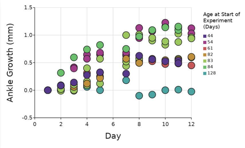
Figure 1. Increase in ankle size (mm) in vivo compared to Day 1. Dots show individual ankle growth compared to the number of days into the experiment. Dots show individual scores for 44 days old mice, (n=1); for 54 days old mice, (n=2); for 61 days old mice, (n=1); for 82 days old mice, (n=1); for 83 days old mice, (n=3); for 84 days old mice, (n=1); for 128 days old mice, (n=1) Figure by authors
There was no significant difference in ankle growth in vivo between Piezo+ and Piezo- mice with the mouse that was 128 days old at the start of the experiment excluded (p = 0 90; ANCOVA, Figure 2) This mouse was excluded for all subsequent in vivo analyses
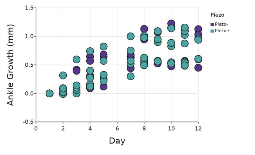
Figure 2. Increase in ankle size (mm) in vivo compared to day 1. Purple dots are Piezo+ mice (n = 5) and teal are Piezo- mice (n = 4) One Piezomouse was excluded due to age Figure by authors Clinical scores of ankles in vivo
Ankles of mice were assigned clinical scores based on the level of inflammation observed by trained researchers over the course of 11 days from the start of K/B.g7 serum treatment. There was no significant difference (p = 0.32; two-way
ANOVA, Figure 3) in ankle clinical score in vivo between Piezo+ and Piezo- mice. For this analysis, the 128-day-old mouse was removed
Bone erosion
Scores of bone erosion were assigned to ankles stained with H&E from Piezo+ and Piezo- mice collected after 11 days of K/B g7 serum treatment (Figure 4). There was no statistically significant (p = 1.00; Mann-Whitney U, Figure 4) difference in bone erosion presence as evaluated by the SMASH protocol and observed with hematoxylin and eosin staining between the Piezo+ and Piezo- mice
Cartilage erosion
Scores of cartilage erosion were assigned to ankles stained with Safranin O from Piezo+ and Piezo- mice collected after 11 days of K/B.g7 serum treatment There was no statistically significant (p = 0 91; Mann-Whitney U, Figure 5) difference in cartilage erosion presence as evaluated by the SMASH protocol and observed with hematoxylin and eosin staining between the Piezo+ and Piezo- mice.
TRAP staining
There was no statistically significant (p = 0 51; Mann-Whitney U, Figure 6) difference in osteoclast presence as evaluated by the SMASH protocol and observed with TRAP staining between the Piezo+ and Piezo- mice.
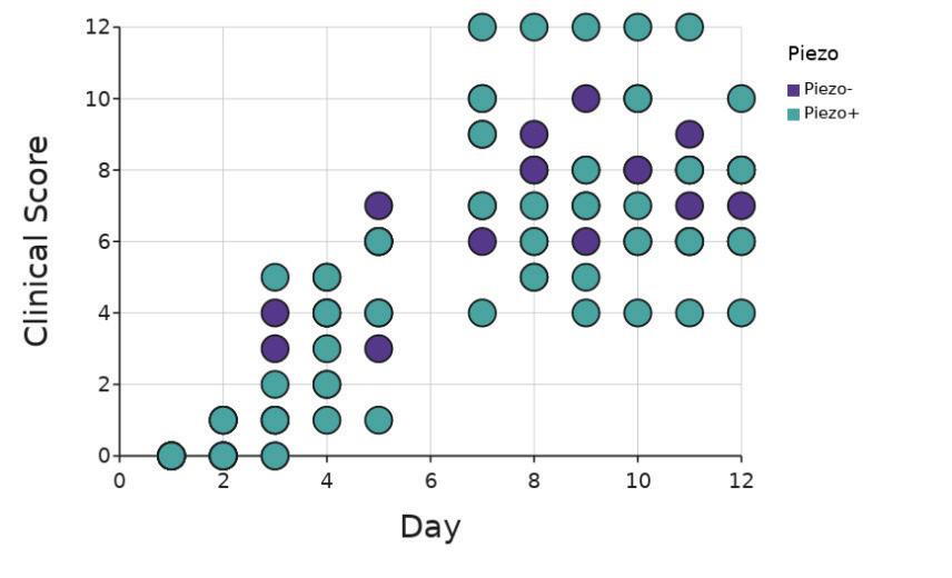
Figure 3. Total ankle clinical score in vivo. Purple circles are Piezo+ mice (n = 5) and teal are Piezomice (n = 4) One Piezo- mouse was excluded due to age Figure by authors
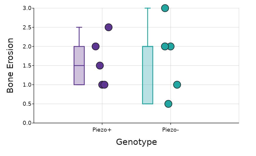
Figure 4. Bone erosion score separated by genotype. Box whiskers plot shows the median value (line), interquartile range (box), and the extent of the data (whiskers above and below at min/max data points). Dots show individual scores for Piezo+ (n = 5) and Piezo- (n = 5) Figure by authors
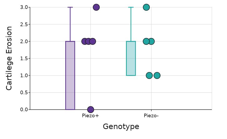
Fgenotype. Box whiskers plot shows the median value (line), interquartile range (box), and the extent of the data (whiskers above and below at min/max data points) Dots show individual scores for Piezo+ (n = 5) and Piezo- (n = 5). Figure by authors.
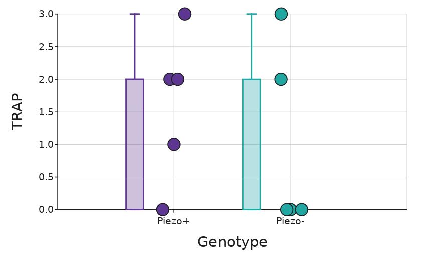
Figure 6. TRAP score separated by genotype. Box whiskers plot shows the median value (line), interquartile range (box), and the extent of the data (whiskers above and below at min/max data points) Dots show individual scores for Piezo+ (n = 5) and Piezo- (n = 5) Figure by authors
Graham Bailey and Samantha Dvorak
Heart data
A statistically significant difference in mitral valve thickness was initially observed between Piezo+ and Piezo- mice (p < .05; Mann-Whitney U; data not shown) However, this difference was entirely due to the inclusion of the Piezomouse that was significantly older, at 128 days, than the other mice, which had ages ranging from 44 to 83 days at collection. This mouse had a significantly thicker mitral valve than all other mice except for the one mouse 82 days old, regardless of genotype (p< 05; ANOVA post-hoc Tukey's range test, Figure 7) Accordingly, this mouse was removed from further analysis. After exclusion of this mouse, there was no significant difference in mitral valve thickness between Piezo+ and Piezo- mice (p = 0 20; Mann-Whitney U; Figure 8)
Discussion
We found no statistically significant differences in any of the scoring of the in vivo ankle growth, the visibly arthritic qualities of the ankles and feet or the stained ankle sections scored for synovial inflammation, bone erosion, cartilage erosion, and osteoclast presence between the Piezo+ and Piezo- mice. Based on our results we can not conclude that PIEZO1 has any impact on the development or course of arthritis in mice given a K/Bg 7 serum transfer Our data and results also indicate that, as expected, the removal of Piezo1 has no effect on the morphology of the mitral valve in mice.
Limitations
We are cautious about concluding that there is no impact, due to some limitations of this preliminary investigation One limitation is that the sample size of mice we used was relatively small: only 10 mice, five Piezo+, and five Piezo-. There was also a wide range of ages that caused some variability in the data One outlier was removed due to its older age, however, there was still a lot of remaining variability in the data Though this variability didn’t appear connected to their ages, there were Piezo+ and Piezo- mice that were not fully age-matched at the onset of the experiment
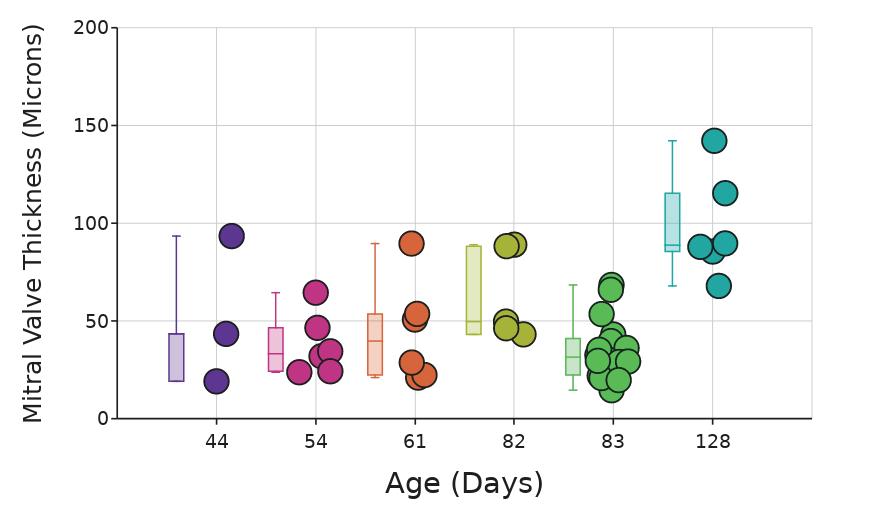
Figure 7. Thickness of the mitral valves (µm) at each age. Box whiskers plot shows the median value (line), interquartile range (box), and the extent of the data (whiskers above and below at min/max data points) Dots show individual scores for 44 days old mice: mouse B, (n=3); for 54 days old mice: mouse H, (n=3) and mouse I, (n=3); for 61 days old mice: mouse E, (n=6); for 82 days old mice: mouse A, (n=5); for 83 days old mice: mouse C, (n=6), mouse D, (n=6), and mouse F, (n=6); for 128 days old mice: mouse G, (n=6) Figure by authors
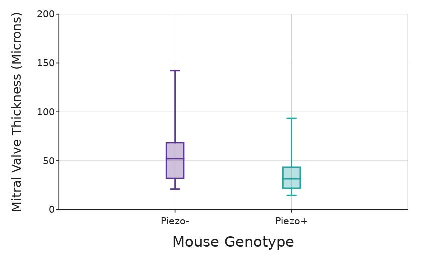
Figure 8. Thicknesses of the mitral valves (µm) compared to the mouse genotype. Box whiskers plot shows the median value (line), interquartile range (box), and the extent of the data (whiskers above and below at min/max data points) Dots show individual scores for Piezo+ mice: mouse A, (n=5), mouse B, (n=3), mouse C, (n=6), and mouse D, (n=6); and Piezo- mice: mouse E, (n = 6), mouse F, (n=6), mouse G, (n=6), mouse H, (n=3), and mouse I, (n=3) Figure by authors
It’s also possible that PIEZO1 may play a different role in human RA or in mouse arthritis not induced by K/Bg.7 serum.
Future work
Additional research will need to be done before PEIZO1 can be conclusively excluded as a possible factor Future work should include more
mice in experiments and age-matching within samples. Other models could include collagen-induced polyarthritis (CIA) and the IL-1RA knockout model In the CIA model, arthritis develops in multiple joints after immunization with cartilage-specific collagen II (Caplazi & Diehl, 2014). This produces immunoreactivity to type II collagen, which is also observed in human rheumatoid arthritis Additionally, it shares other commonalities with human RA, including the development of rheumatoid factor and anti-citrullinated peptide antibodies (ACPAs) that circle the body during the disease. Its similarity in mechanisms to human RA, makes it an ideal model for further defining the role of Piezo1 Another viable option is the IL-1RA knockout (KO) model which presents very similarly to human RA. IL-1RA knockout mice also have rheumatoid factor, develop autoantibodies to type II collagen, and are T-cell dependent, like in human arthritis (Caplazi & Diehl, 2014) Its T cell dependency in particular makes it an interesting model for further studying Piezo1 because it involves the adaptive immune system similar to human RA Since our data did not indicate that PIEZO1 is involved in worsening rheumatoid arthritis in the K/B g7 serum-transfer model, this research may narrow down potential targets for stopping the devastating effects of this disease. However, completely ruling out the role of pressure-sensing proteins would necessitate further research into their involvement in rheumatoid arthritis, and further defining the role of PIEZO1 within this and other mouse models.
Beyond PIEZO1, other pressure-sensing targets must be studied to determine any potential roles in worsening inflammation. One of these targets could include Piezo2, a mechanosensitive ion channel, which has been associated with other inflammatory diseases (Liu et al , 2022) Due to the observed correlations between pressure-sensing proteins and inflammation, further research must be done to understand these interactions fully.
Graham Bailey and Samantha Dvorak
Conclusions
Despite previous observations of pressuresensing proteins having a role in inflammatory diseases, there was no observable connection in our data Since PIEZO1 did not appear to be involved in the development of rheumatoid arthritis, it’s possible that PIEZO1 does not play a crucial role in developing the disease. This could be used to rule out pathways and narrow down effective targets for stopping the devastating effects of rheumatoid arthritis
This research is a first step towards ruling out one potential pathway for the development of rheumatoid arthritis Furthermore, the observation that Piezo1’s removal did not appear to impact the mitral valve in this model will allow for greater confidence in its removal as a way to evaluate PIEZO1’s potential implications in other related autoimmune diseases, like rheumatic heart disease
Acknowledgments
We would like to thank Dr Kati Kragtorp for guiding us through science research and creating this paper. We would also like to thank Dr. Bryce Binstadt for the opportunity to work in his lab and for his support throughout our research Additionally, we would like to thank Jenn Auger, Alyssa Peck, and Charles Rolls for their time spent teaching us these laboratory techniques and their assistance throughout our time in the lab
References
Autoimmune Disease An overview | ScienceDirect Topics (n d ) Retrieved July 21, 2024, from https://www sciencedirect com/topics/immunology-and-microbiolo gy/autoimmune-disease#: :text=Autoimmune%20diseases%20are %20a%20set,high%20financial%20costs%20%5B1%5D
Autoimmune disorders found to affect around one in ten people | University of Oxford (2023, May 6) https://www ox ac uk/news/2023-05-06-autoimmune-disorders-fou nd-affect-around-one-ten-people
Breed, E R , & Binstadt, B A (2015) Autoimmune valvular carditis Current Allergy and Asthma Reports, 15(1), 491 https://doi org/10 1007/s11882-014-0491-z
Caplazi, P , & Diehl, L (2014) Histopathology in Mouse Models of Rheumatoid Arthritis In S J Potts, D A Eberhard, & K A Wharton, (Eds ), Molecular Histopathology and Tissue Biomarkers
in Drug and Diagnostic Development (pp 65–78) Springer New York https://doi org/10 1007/7653 2014 20
Chen, M , Lam, B K , Kanaoka, Y , Nigrovic, P A , Audoly, L P , Austen, K F , & Lee, D M (2006) Neutrophil-derived leukotriene B4 is required for inflammatory arthritis The Journal of Experimental Medicine, 203(4), 837–842 https://doi org/10 1084/jem 20052371
Galvin, J E , Hemric, M E , Ward, K , & Cunningham, M W (2000) Cytotoxic mAb from rheumatic carditis recognizes heart valves and laminin The Journal of Clinical Investigation, 106(2), 217–224 https://doi org/10 1172/JCI7132
Gorton, D , Blyth, S , Gorton, J G , Govan, B , & Ketheesan, N (2010) An alternative technique for the induction of autoimmune valvulitis in a rat model of rheumatic heart disease Journal of Immunological Methods, 355(1–2), 80–85 https://doi org/10 1016/j jim 2010 02 013
Hayer, S , Vervoordeldonk, M J , Denis, M C , Armaka, M , Hoffmann, M , Bäcklund, J , Nandakumar, K S , Niederreiter, B , Geka, C , Fischer, A , Woodworth, N , Blüml, S , Kollias, G , Holmdahl, R , Apparailly, F , & Koenders, M I (2021) “SMASH” recommendations for standardised microscopic arthritis scoring of histological sections from inflammatory arthritis animal models Annals of the Rheumatic Diseases, 80(6), 714–726 https://doi org/10 1136/annrheumdis-2020-219247
Liu, H , Hu, J , Zheng, Q , Feng, X , Zhan, F , Wang, X , Xu, G , & Hua, F (2022) Piezo1 Channels as Force Sensors in Mechanical Force-Related Chronic Inflammation Frontiers in Immunology, 13, 816149 https://doi org/10 3389/fimmu 2022 816149
Marijon, E , Mirabel, M , Celermajer, D S , & Jouven, X (2012) Rheumatic heart disease Lancet (London, England), 379(9819), 953–964 https://doi org/10 1016/S0140-6736(11)61171-9
Monach, P , Hattori, K , Huang, H , Hyatt, E , Morse, J , Nguyen, L , Ortiz-Lopez, A , Wu, H -J , Mathis, D , & Benoist, C (2007) The K/BxN mouse model of inflammatory arthritis: Theory and practice Methods in Molecular Medicine, 136, 269–282 https://doi org/10 1007/978-1-59745-402-5 20
Osinski, V , Yellamilli, A , Firulyova, M M , Zhang, M J , Peck, A L , Auger, J L , Faragher, J L , Marath, A , Voeller, R K , O’Connell, T D , Zaitsev, K , & Binstadt, B A (2024) Profibrotic VEGFR3-Dependent Lymphatic Vessel Growth in Autoimmune Valvular Carditis Arteriosclerosis, Thrombosis, and Vascular Biology, 44(4), 807–821 https://doi org/10 1161/ATVBAHA 123 320326
Raizada, V , Williams, R C , Chopra, P , Gopinath, N , Prakash, K , Sharma, K B , Cherian, K M , Panday, S , Arora, R , Nigam, M , Zabriskie, J B , & Husby, G (1983) Tissue distribution of lymphocytes in rheumatic heart valves as defined by monoclonal anti-T cell Antibodies The American Journal of Medicine, 74(1), 90–96 https://doi org/10 1016/0002-9343(83)91124-5
Smolen, J. S., Aletaha, D., Barton, A., Burmester, G. R., Emery, P., Firestein, G S , Kavanaugh, A , McInnes, I B , Solomon, D H , Strand, V., & Yamamoto, K. (2018). Rheumatoid arthritis. Nature Reviews Disease Primers, 4(1), 1–23 https://doi.org/10.1038/nrdp.2018.1
Xie, L , Wang, X , Ma, Y , Ma, H , Shen, J , Chen, J , Wang, Y , Su, S , Chen, K , Xu, L , Xie, Y , & Xiang, M (2023) Piezo1
(Piezo-Type Mechanosensitive Ion Channel Component 1)-Mediated Mechanosensation in Macrophages Impairs Perfusion Recovery After Hindlimb Ischemia in Mice Arteriosclerosis, Thrombosis, and Vascular Biology, 43(4), 504–518 https://doi org/10 1161/ATVBAHA 122 318625
Abigail Endres and Selena Qiao
Tur f Trouble:
Does the DEET in bug repellent really kill grass? Year II
Abigail Endres, Selena Qiao
Introduction
DEET, or N, N-diethyl-meta-toluamide, is a chemical that is typically the active ingredient in most bug spray repellents DEET is a neurotoxin believed to affect the olfactory receptors in insects and vertebrates, inhibiting an insect’s ability to locate humans (Martinez et al., 2016). DEET is extremely effective as an insect repellent; around one-third of the U S population annually uses DEET to prevent mosquito-borne diseases like malaria and tick-borne diseases like Lyme disease (US EPA, 2013a).
DEET was originally developed by the U S Army in 1957 and registered for public use in 1964 (US EPA, 2013a). The U.S. Environmental Protection Agency (EPA) reviews each pesticide at least every 15 years to ensure it is generally safe for public use (US EPA, 2013b) DEET was reviewed in 1998 and again in 2014 The EPA found that DEET is safe for humans to use and is slightly toxic to birds and fish (Reregistration Eligibility Decision (RED) DEET, 1998). However, this report did not examine the potential effects on the environment, stating that “environmental risk assessments are not conducted for pesticides with exclusively indoor use patterns” (Reregistration Eligibility Decision (RED) DEET, 1998).
Anecdotal evidence suggests that bug sprays containing DEET damage grass (DEET Is Lethal to Grass; Take Care When Using, 2016; “Is DEET Really All That Bad?,” 2019; Graedon & Graedon, 2007) In particular, this is a problem for golf courses Certain areas of golf courses, such as tee boxes and greens, are more sensitive and susceptible to damage due to short mowing heights. Repairing damage caused by bug spray is costly, not only in money but also in water and other natural resources Although there are no

rigorous peer-reviewed studies on the topic, there are a few informal studies and records of observations posted online addressing the subject In a short article from Michigan State, a professor states how they have observed that bug sprays kill grass (Frank, 2013) A brief study from Kansas State examined the impact of different commercial bug sprays on perennial ryegrass, with four replicants for each treatment group The study found that the bug sprays with a higher DEET concentration caused greater grass damage (Hoyle, 2017). A short report from Iowa State University tested the impact of different commercial chemical sprays on grass commonly used in golf greenways A researcher sprayed patches of bentgrass with bug sprays containing DEET and bug sprays without DEET Each application was repeated on three different patches, approximately a week apart. The researchers concluded that bug sprays containing DEET caused immediate grass damage that took upwards of three weeks to recover The patches sprayed with non-DEET bug spray showed no signs of damage (Christians, 2015). While these observations and findings are interesting, the research was not conducted very rigorously. Furthermore, while looking into the toxicity of DEET on plants, we were unable to find any other scientific reports on the subject
To our knowledge, no peer-reviewed study exists that investigates the toxicity of DEET to any plants We did find two papers that examined the environmental toxicity of DEET. A study reported that DEET that enters the environment through runoff poses a low environmental risk (Weeks et al , 2012) A study examined the potential toxicological effects of DEET in algae in environments with low water circulation They concluded that oxygen flux was significantly i nhibited when exposed to DEET, providing preliminary evidence that details the toxic effects of DEET (Martinez et al , 2016)
In Year One of this project (2023/2024), one of the authors (Qiao) tested how commercial insect repellents containing DEET impacted different types of grass This study used four treatment groups: 7% DEET, 25% DEET, a natural alternative containing lemongrass oil, and a control where no treatment was sprayed. The study tested perennial ryegrass, Kentucky bluegrass, and creeping bentgrass, each with six pots for each treatment group Perennial ryegrass and creeping bentgrass were tested because they are commonly used on golf courses, and Kentucky bluegrass is a common lawn grass in the northern United States (Bauer, n.d.). Qiao found that DEET affected all three types of grass in a dose-dependent manner, with the bug spray with 25% DEET damaging the grass the fastest However, the grass treated with 7% DEET bug spray eventually reached the same level of damage as the grass treated with the bug spray containing 25% DEET
Safety Data sheets for the 7% and 25% DEET insect repellent used in the first year of this study reported 60-100% and 30-60% respectively of the carrier ethanol in each solution as the only other major ingredient (OFF! Deep Woods Insect Repellent VII, Long Lasting Protection, Pump Spray, 2021; OFF! FamilyCare Insect Repellent IV, Unscented with Aloe Vera, Pump Spray, 2015) The 25% DEET bug spray had a lower concentration of ethanol, suggesting that it was the DEET and not the ethanol that was damaging the grass. However, this hypothesis was not tested in year one. Another limitation of the original study was that the grass damage was analyzed using a qualitative ranking system, meaning that the analysis could have been biased and subject to human error. Furthermore, the method of spraying wasn’t standardized, leading to inconsistent coverage of bug spray. Finally, the photos were taken with an iPhone camera, which automatically adjusted the color and contrast of the photo, leading to inconsistent lighting.
This year, our goals were to identify whether DEET or ethanol damaged the grass, if grass treated with DEET would recover, if the addition of DEET directly to the soil impacted the health
of the grass, and if DEET exposure to grass in an outdoor environment would impact the level of grass damage Lastly, we investigated DEET’s mechanism of toxicity
Materials and Methods
Planting and treatment standardization
One issue encountered in Year I of this study was that the unevenness of the soil during planting caused the grass in the pots to grow in a non-uniform manner, such that the grass was distributed unevenly
To address this problem, we designed a soil flattening tool (Figure 1) using the SolidWorks (Dassault Systèmes) computer-aided design (CAD) software We then 3D printed the tool on a Prusa i3 MK3S+ 3D Printer After the soil was added to the pot, the soil flattening tool was moved in a light circular motion above the soil. This act ensured that there was a firm and flat surface on which the seeds could be placed
Another issue in Year I was standardizing the angle and distance of the spray bottle to the grass To address this issue, we designed and 3D-printed a tool for a uniform method of spraying grass pots The two components of the tool were a pot holder for the grass and a rod that guided the user to hold the spray bottle at the correct angle and height. The pot holder was later used as the circular spraying template during the outdoor turfgrass plot experiments (Figure 1)
Analysis of images for indoor plants
We used a Canon EOS Rebel T7i Digital SLR camera to take photos of the grass. The pots of grass were moved to a room with consistent lighting and no windows The camera was positioned on a tripod at an overhead angle so that the images were taken from the top. A lamp was placed near the set-up to improve the lighting. The pots of grass were placed under the camera in a marked circle one by one so that the position of the pots in the image remained constant
The images were analyzed in ImageJ (Schneider et al., 2012). An ImageJ macro for extracting information about color in images was used to measure the area of the healthy grass in each picture (Strock, 2021) Since the damaged grass was a distinct yellow compared to the normal green color, we set parameters for color thresholds that would select and create a mask for the green portions of the grass Analyzing the mask generated the area of the healthy grass in pixels Some experimentation was done to determine the best parameters for the color threshold since some thresholds would incorrectly mask the background instead of the grass The HSB color space was used along with the Minimum thresholding method, which produced the best mask coverage results
Treatment of outdoor plots
Perennial ryegrass (Lolium perenne), creeping bentgrass (Agrostis stolonifera), and Kentucky bluegrass (Poa pratensis) plots were provided by the University of Minnesota Turfgrass Research Center, and two 1 by 1-meter plots were used for each type of grass. Within each plot of grass, there were four treatment groups with four replicants each, which totaled 16 treatments within each plot A circular spraying template was used to treat sections of grass at the 20, 40, 60, and 80 cm marks within the 1 x 1 meter plot At each spot, the grass was sprayed from four angles around the circular treatment area (0, 90, 180, and 270 degrees) with either 60% ethanol, 2 5% DEET, 15% DEET, or 25% DEET
Collection and analysis of images for outdoor plots
The outdoor plots were photographed from the top at an overhead angle One image was taken per plot, so there were two pictures per grass type. The benchmark used to standardize the photos were four flags that marked the corners of each plot The images were analyzed in ImageJ using the same macro template from the indoor experiments Because the plots were outdoors, the lighting in each picture varied based on the weather. Thus, we adjusted the color parameters for each image according to its lighting conditions Each photo of a single plot contained
Abigail Endres and Selena Qiao
sixteen treatments, each image was cropped into sixteen 400x400 pixel photos of the individual treatments, with the circle of treatment positioned in the center of each photo The damaged treatment circles were yellow while the background of healthy grass was green, so the new thresholds selected and masked the yellow grass. The area of the mask was then recorded for every cropped image
Sample collection and preparation for metabolomics analysis
Twelve pots of grass were grown in the standard setup at our school Once the grass had grown for three weeks, we transferred the tray of grass to a controlled growth chamber where it was stabilized for two weeks. The grass remained in the growth chamber throughout sampling. Six pots of grass were treated with ethanol and the other six were treated with 15% DEET
Samples were collected immediately after treatment and for five days after treatment In a line across the pot, we plucked 40 blades of grass, and then, perpendicular to that, we plucked another 40 blades of grass. If the grass was longer than 2.5 cm, we reduced the number of blades we selected to collect approximately 200 cm of grass The blades of grass were then placed into a test tube, which was then placed on dry ice
To prepare for liquid chromatography mass spectrometry (LC-MS) analysis, the tubes were transported out of the freezer in a cooler box with dry ice One tungsten bead was then placed within each sample tube to help beat the plant tissue in the tube. A stock solution of methanol with 10% formic acid was then added to each tube based on the mass of the grass sample Each sample tube was then secured into the Geno/Grinder The tubes ran through the Geno/Grinder for five minutes at 150 rpm. The tubes were then placed into the microcentrifuge for 5 minutes at 1400 rpm
LC-MS methods
A trained researcher then performed LC-MS on the samples to create a map of how the metabolome of the grass changes after DEET
exposure and supplied the following information about these methods (K. Freund, personal communication): Metabolomic profiles were obtained using C18 reversed-phase ultraperformance liquid chromatography–electrospray ionization–hybrid quadrupole –orbitrap mass spectrometer (Ultimate® 3000 HPLC, Q Exactive™, Thermo Fisher Scientific, Waltham, MA, USA) with an autosampler and with a sample vial block maintained at 4 °C Chromatographic separations were carried out on an Acquity reversed-phase C18 HSS T3 1.8 µm particle size, 2.1 mm × 100 mm column (Waters, Milford, MA, USA) with column temperature 40 °C, flow rate 0 400 mL/min, and 1 µL injected A 16 min gradient using mobile phases A: 0 1% formic acid in water and B: 0.1% formic acid in acetonitrile was run according to the following gradient elution profile: initial 2% B, 0.5 min 2% B, 15 min 98% B, 0 5 min 2% B The MS conditions used were full scan mass range 125-1800 m/z, resolution 70 000, desolvation temperature 350 °C, spray voltage 3800 V, auxiliary gas flow rate 20, sheath gas flow rate 50, sweep gas flow rate 1, S-Lens RF level 50, and auxiliary gas heater temperature 300 °C Xcalibur™ software version 2 1 (Thermo Fisher Scientific, Waltham, MA, USA) was used for data collection and chromatogram visualization. Sample analysis order was randomized across the entire sample set
Data processing and analysis
A trained researcher also performed the analysis of LC-MS results and supplied the following information about these methods (K. Freund, personal communication): The ProteoWizard tool MSconvert (Chambers et al , 2012) was used to convert raw files to mzML format for positive and negative ionization data MZmine 2 version 2.53 (Pluskal et al., 2010) was used to process chromatographic data through mass detection, chromatogram building, chromatogram deconvolution, and deisotoping steps Alignment of samples was attained through the RANSAC aligner tool, and gap filling using Same RT and m/z range gap filler algorithm was
performed to detect missing peaks. Non-peak shape features were removed after visual inspection and 1692 unique positive mode and 838 unique negative mode features were detected based on the combination of distinct m/z and retention time. Positive and negative datasets were exported to .csv file format and combined for analysis in RStudio (Posit Team, 2023) Data were log2-transformed before multivariate statistical analyses and were visualized using principal component analysis (PCA) using the R package ropls (Thévenot et al., 2015).
Results
Determination of Dose-Response of Grass to DEET Exposure
We initially conducted a pilot experiment with 10 pots of silver sport perennial ryegrass that had been cut to 2 cm One pot was sprayed with DI water, one was exposed to 100% DEET, two were exposed to 60% ethanol, two were exposed to 60% ethanol with 5% DEET, two were exposed to 60% ethanol with 15% DEET, and two were exposed to 60% ethanol with 25% DEET Images of the grass were captured and analyzed for damage All the grass sprayed with DEET in this pilot experiment died within three days of treatment (Figure 1).
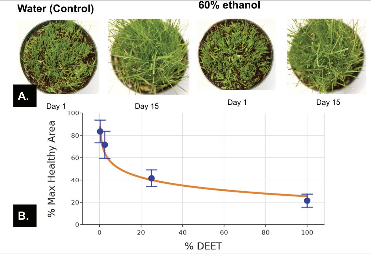
Figure 1. A) Representative images of grass treated with water and 60% ethanol on day 1 (immediately after treatment) and 15 days after treatment B) Percent of the maximum possible healthy (green) area of grass measured in images with different levels of DEET treatment one day after treatment The graph displays the mean and standard deviation of the percentage of healthy grass in pots treated with
0.25% DEET, 2.5% DEET, 25% DEET, and 100% DEET, one day after treatment All DEET solutions other than 100% DEET also contained 60% ethanol The percentage of healthy grass was calculated by dividing the area of the green grass in the DEET treatment groups over the “maximum healthy area”, or the average area of healthy grass in the pots treated with 60% ethanol n = 4 for all treatment groups Figure by authors
Based on these results, we decided to use lower concentrations of DEET to establish the lowest concentration of DEET that would damage the grass We kept the 100% DEET and 60% ethanol with 25% DEET solutions and replaced our other DEET treatments with 60% ethanol with 2.5% DEET and 60% ethanol with 0.25% DEET. The water-only control and the 60% ethanol solution were kept for this full dose-response experiment We planted 24 pots of perennial ryegrass so that there were 4 replicants of all the 6 treatments that were used in this experiment. There was no significant difference in damage between the grass exposed to the 60% ethanol solution and the grass exposed to water (data not shown) Accordingly, 60% ethanol was used as a control for subsequent data analysis
Within one day of exposure, pots treated with higher levels of DEET showed increased levels of damage, indicating that DEET damaged grass in a dose-dependent relationship (Figure 1) Based on this data, we calculated an effective dose to damage 50% of the grass (ED50) of 9 7% DEET
The area of healthy (green) grass over 15 days of exposure was not significantly different between pots treated with 60% ethanol and pots treated with 0 25% DEET (Figure 2, ANOVA, Tukey post-hoc; p = 0 99) This shows that 0 25% DEET does not have any visible effect on grass health. Pots treated with 2.5% DEET displayed a slower increase in green area over 15 days after treatment but had an overall increase in green over the course of the experiment and a majority of the grass was a light green by day 15 (Figure 2) By day 15, pots treated with 25% DEET and 100% DEET had no living grass (Figure 2). Pots treated with 100% DEET solution had no healthy grass by day 3, while 25% DEET-treated
Abigail Endres and Selena Qiao
grass reached that point by day 4 after treatment (Figure 2). We continued to follow the pots from the pilot and full experiments for several weeks after exposure No new growth was observed in pots treated with 5% DEET or higher, even up to 30 days after exposure (data not shown). In further trials, DEET treatment was immediately followed by either wiping the grass or spraying it with water in an attempt to reduce the damage, however, these interventions had no measurable effect on the level of grass damage (data not shown).
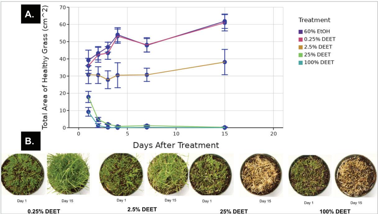
Figure 2. A) Total area of healthy (green) grass (cm^2) measured in images over 15 days after treatment The graph displays the mean and standard deviation of the percentage of healthy grass in pots treated with 60% ethanol, 0 25% DEET, 2 5% DEET, 25% DEET, and 100% DEET, one day after treatment All DEET solutions other than 100% DEET also contained 60% ethanol n = 4 pots for all treatment groups. B) Representative images of grass treated with 0 25% DEET, 2 5% DEET, 25% DEET, and 100% DEET group, 1 day after treatment and 15 days after treatment Figure by authors
Measurement of the Impact of Different DEET Exposure Methods
We experimented with alternate methods of DEET exposure to test if indirect exposure through the soil would affect grass health The grass was planted with a gap in the middle so that there was a circle of soil that was surrounded by grass. Using a pipette, the soil in the middle was exposed to different concentrations of DEET solutions Pictures of the grass were taken daily over the span of a week There was no significant difference between the green area in the grass treated with water and the grass treated with ethanol (data
not shown). Damage was confined to the area directly surrounding the treated soil (data not shown)
The area of healthy (green) grass was significantly different between the 60% ethanol control group and the 100% DEET treatment group on day 6 (data not shown) While the other treatment groups showed an initial decrease in the area of healthy grass for the first three days after treatment, this difference was not significant, and the area of healthy grass reached the same point as the control group (data not shown)
DEET Exposure in an Outdoor Environment
To understand the impact of DEET exposure on outdoor grass, turfgrass plots were provided by the Watkins Labs at the University of Minnesota to conduct an outdoor version of the ethanol and DEET experiment Three species of grass (perennial ryegrass, Kentucky bluegrass, and creeping bentgrass) were treated with solutions of 25% DEET and 60% ethanol, 15% DEET and 60% ethanol, 2.5% DEET and 60% ethanol, and 60% ethanol The purpose of this experiment was to confirm the existence of a dosedependent relationship between grass damage and DEET concentrations outdoors Since the 0.25% DEET treatment group had no visible effect on grass health and the 100% DEET treatment group caused similar amounts of damage compared to the 25% DEET treatment group, the 0 25% and 100% concentrations were not included. Instead, 15% DEET was used as an intermediate concentration between 2.5% and 25% DEET.
Pictures of the grass were taken daily over the span of a week. Damage was observed in treated areas within one day of treatment in the creeping bentgrass (data not shown), perennial ryegrass, and Kentucky bluegrass (data not shown) In the creeping bentgrass plots, compared to the 60% ethanol control, there was a significant increase in the area of damaged bentgrass exposed to 25% DEET, 15% DEET, and 2.5% DEET on days 1 through 7 (data not shown ), though there appeared to be some recovery in the grass
exposed to 15% DEET by day 7 (Figure 11). A similar pattern was observed in perennial ryegrass and Kentucky bluegrass (data not shown) A small amount of damage was noted in the 60% ethanol control sections at the spots where the template tool used during treatments was touching the bentgrass, but not in the middle area where the ethanol was actually sprayed (Figure 10) Although efforts were made to thoroughly clean the template tool between treatments, this damage is more consistent with residual DEET on the template tool, rather than damage resulting from the ethanol. We found that the outdoor grass was able to recover at a faster rate than the indoor grass This could have been a result of the weather or watering schedule, which may have lessened DEET’s effect on the grass. Additionally, differences in the uncontrolled lighting outdoors increased the potential inconsistency in image analysis.
Assessment of Metabolomic Differences of Grass Exposed to DEET
Using equipment provided by the University of Minnesota, we investigated how DEET exposure changes the metabolome of grass, which in turn could help determine how DEET damages the grass. Pots of grass were treated with either 60% ethanol or 15% DEET using our standard procedure The 15% DEET treatment group was used to ensure that gradual damage occurred over a period of four days Samples were collected prior to treatment, 1 hour after treatment, and one, two, three, and four days after treatment, then processed for LC-MS analysis following standard procedures An untargeted metabolomics approach was used, involving simultaneous measurement and relative quantification of all known and unknown metabolites. Within each sample, all detected ions were scaled to the most abundant ion to quantify phytochemical content Principal component analysis (PCA) was used to analyze the effect of treatment on the metabolic profile of the grass. PCA is a common method used to investigate patterns and correlations in complex metabolomic data sets There was no difference in the metabolomic profiles of samples prior to
treatment with either 60% ethanol or DEET (data not shown).
Major differences were apparent in the metabolomic profiles of grass exposed to DEET as compared to 60% ethanol as early as 1 hour after exposure (Figure 3), and the metabolic profiles of grass exposed to DEET, but not 60% ethanol (data not shown), displayed significant shifts each day from day zero to day one (data not shown), with less separation in metabolic profiles on days two through four (data not shown), at which times the DEET-treated grass appeared to have mostly died (data not shown).
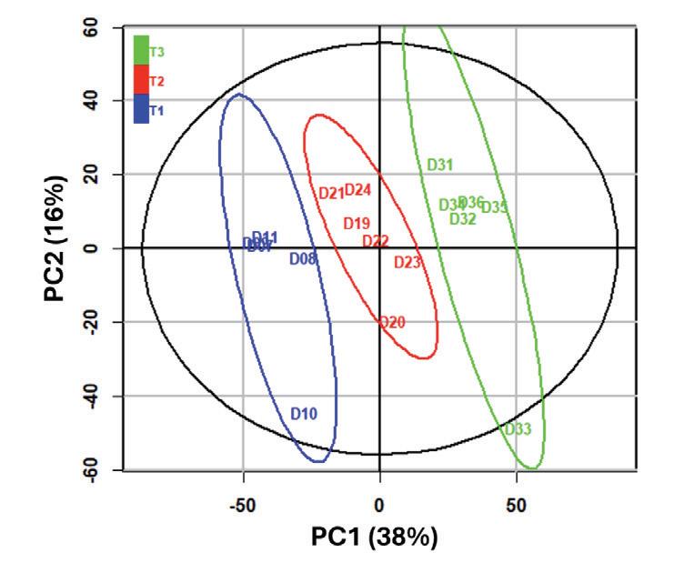
Figure 3. Samples prior to treatment with 15% DEET (blue), 1 hour after treatment (red) and 1 day after treatment (green). The percent of variation explained by each principal component is shown on each axis Figure by K Freund
Discussion
We determined that DEET kills grass in a dose-dependent manner in both a controlled, indoor environment and on three different species of grass in an outdoor environment We found the grass that died from DEET exposure did not recover up to 30 days after exposure. We demonstrated that grass next to DEET-exposed soil caused seemingly identical damage to grass sprayed with DEET This shows that the mechanism of DEET toxicity does not require direct application to the blade's surface. This experiment suggests that DEET is absorbed by the roots, causing damage to grass in the surrounding area Furthermore, an untargeted metabolomics analysis of treated grass revealed
Abigail Endres and Selena Qiao
significant differences in the metabolomes of treated grass within 1 hour of DEET application, indicating a rapid toxic mechanism In addition, the analysis revealed significant differences between the metabolomes of the time-sampled grass, indicating that DEET affects grass in a time-dependent manner. It can be concluded that DEET toxicity is caused by a change in the grass metabolome; however, identifying the specific metabolomic pathway responsible for the change requires further analysis
Future investigations will examine the toxic mechanism behind DEET’s effect on grass By continuing metabolomics analysis, we can get a deeper look into what specific features in the grass are changing after being exposed to DEET. The previous year, we conducted a time-lapse experiment using a camera to film a pot of grass after it had been treated with DEET Over the course of 24 hours, the blades of grass seemed to shrink in width and shrivel slightly, suggesting that the grass was losing water as a result of the DEET treatment. To test this hypothesis, we plan to use a fluorescence microscope to capture changes in stomata stained with DAPI A previous study conducted on algae indicated that photosynthesizing organisms might be more sensitive to DEET than non-photosynthetic microorganisms (Martinez et al., 2016). Thus, additional research should expand the scope to plants other than grass, as they are also possibly susceptible to DEET exposure Overall, this is a novel finding that opens up new, unexplored questions in the field of plant toxicology and indicates that, though the use of DEET-based bug sprays is necessary for protection from disease-causing insects, care should be taken when applying it to avoid contacting plants in the area.
References
Bauer, S (n d ) Minnesota Home Lawns University of Minnesota Extension Turfgrass Science https://turf umn edu/sites/turf umn edu/files/files/media/turfgrass i nfographic 1 pdf
Chambers, M C , Maclean, B , Burke, R , Amodei, D , Ruderman, D L , Neumann, S , Gatto, L , Fischer, B , Pratt, B , Egertson, J , Hoff, K , Kessner, D , Tasman, N , Shulman, N , Frewen, B , Baker, T A , Brusniak, M -Y , Paulse, C , Creasy, D , Mallick, P
(2012) A cross-platform toolkit for mass spectrometry and proteomics Nature Biotechnology, 30(10), 918–920
https://doi org/10 1038/nbt 2377
Christians, N (2015, August 25) Mosquito Spray Can Kill Grass Turfgrass
https://www extension iastate edu/turfgrass/blog/dr-nick-christians/ mosquito-spray-can-kill-grass
Deep Woods OFF killed the grass- Yikes! (2011, July 9) https://windsorpeak com/vbulletin/showthread php?403732-DeepWoods-OFF-killed-the-grass-Yikes!&p=3193658
DEET is lethal to grass; take care when using (2016, July 28)
Longview News-Journal
https://www news-journal com/features/atplay/deet-is-lethal-to-gra ss-take-care-when-using/article 7cba0999-c391-5f0d-b291-c20a42 cf5352 html
Frank, K (2013, May 30) Mosquito repellent can damage turf MSU Extension
https://www canr msu edu/news/mosquito repellent can damage t urf
Graedon, J , & Graedon, T (2007, August 28) Dead grass raises question on DEET safety | The Spokesman-Review https://www spokesman com/stories/2007/aug/28/dead-grass-raises -question-on-deet-safety/
Hoyle, J (2017, June 29) The Effect of Human Insect Repellents on Perennial Ryegrass (Lolium perenne) Growth and Recovery | K-State Turf and Landscape Blog
https://blogs k-state edu/turf/the-effect-of-human-insect-repellentson-perennial-ryegrass-lolium-perenne-growth-and-recovery/
Is DEET Really All That Bad? (2019, August 16) No Mozzie https://nomozzie co uk/is-deet-really-all-that-bad/
Martinez, E , Vélez, S M , Mayo, M , & Sastre, M P (2016)
Acute toxicity assessment of N,N-diethyl-m-toluamide (DEET) on the oxygen flux of the dinoflagellate Gymnodinium instriatum
Ecotoxicology, 25(1), 248–252 https://doi org/10 1007/s10646-015-1564-z
OFF! Deep Woods Insect Repellent VII, Long Lasting Protection, Pump Spray (2021, August 6) Consumer Protection Information
Database
https://www whatsinproducts com/types/type detail/1/24071/stand ard/19-001-855
OFF! FamilyCare Insect Repellent IV, Unscented with Aloe Vera, Pump Spray (2015, February 23) Consumer Protection Information Database
https://www whatsinproducts com/types/type detail/1/16560/stand ard/p%20class=%22p1%22%3Espan%20style=%22color:
Pluskal, T , Castillo, S , Villar-Briones, A , & Orešič, M (2010)
MZmine 2: Modular framework for processing, visualizing, and analyzing mass spectrometry-based molecular profile data BMC Bioinformatics, 11(1), 395 https://doi.org/10.1186/1471-2105-11-395
Reregistration Eligibility Decision (RED) DEET (1998) U S EPA.
https://www3 epa gov/pesticides/chem search/reg actions/reregistr ation/red PC-080301 1-Apr-98.pdf
Schneider, C A , Rasband, W S , & Eliceiri, K W (2012) NIH Image to ImageJ: 25 years of image analysis Nature Methods, 9(7), 671–675 https://doi org/10 1038/nmeth 2089
Strock, C (2021) Protocol for extracting basic color metrics from Images in ImageJ/Fiji Zenodo https://doi org/10 5281/ZENODO 5595203
Thévenot, E A , Roux, A , Xu, Y , Ezan, E , & Junot, C (2015) Analysis of the Human Adult Urinary Metabolome Variations with Age, Body Mass Index, and Gender by Implementing a Comprehensive Workflow for Univariate and OPLS Statistical Analyses Journal of Proteome Research, 14(8), 3322–3335 https://doi org/10 1021/acs jproteome 5b00354
US EPA, O (2013a, July 15) DEET [Overviews and Factsheets] https://www epa gov/insect-repellents/deet
US EPA, O (2013b, August 29) Registration Review Process [Overviews and Factsheets] Registration Review Process https://www epa gov/pesticide-reevaluation/registration-review-pro cess
Weeks, J , Guiney, P , & Ai Nikiforov (2012) Assessment of the environmental fate and ecotoxicity of N,N‐ diethyl ‐ m‐ toluamide (DEET) Integrated Environmental Assessment and Management, 8(1), 120–134 https://doi org/10 1002/ieam 1246
Immune Inter ference
Is aberrant DUX4 expression responsible for the downregulation of MHC class I genes stimulated by IFN-γ?
Abigail Getnick and Kelan McKay
Introduction
The gene Double Homeobox 4 (DUX4) is a transcription factor typically active during early embryonic development that plays an important role in regulating other genes during this period Past this stage, the DUX4 gene is typically repressed by both genetic and epigenetic processes, including DNA methylation and histone modifications. However, derepression caused by genetic mutations or loss of epigenetic silencing can lead to reexpression of DUX4 (Karpukhina et al , 2021) This aberrant DUX4 expression is believed to be the primary driver of muscle degeneration in Facioscapulohumeral Muscular Dystrophy (FSHD), a rare type of progressive muscula r dystrophy (Schätzl et al , 2021) DUX4 has also been found to be re-expressed in many solid cancers, and researchers have suggested that this upregulation may allow cancerous cells to evade detection from the immune system (Smith et al., 2023).
The current consensus is that immune evasion of cancer by the activation of DUX4 is driven by suppression of the Major Histocompatibility Complex class I (MHC I) MHC I refers to a set of genes that encode vital proteins that allow the immune system to detect and respond to foreign pathogens by presenting the immune system with peptide fragments of these pathogens. To do so, MHC I proteins break down intracellular proteins and bring their fragments to the cell ’s surface, allowing for immune cells such as T-cells and Natural Killer (NK) cells to recognize and destroy pathogens, including various bacteria, viruses, and cancer cells (Janeway et al., 2001). In the absence of MHC class I gene expression, diseased cells and other pathogens can more easily evade detection by the immune system For cancer, the suppression of MHC I may allow for undisturbed proliferation. MHC I suppression has also been

found to make developing immunotherapies, such as immune checkpoint blockade, less effective for solid cancers Due to these findings, researchers have reported that upregulating MHC class I genes may allow for more effective application of immunotherapy against solid tumors (Cornel et al., 2020; Pineda & Bradley, 2023)
To study aberrant DUX4 expression, researchers use genetically modified cell lines with Tet-On systems in which doxycycline can be used to control activation of DUX4 transcription To create these Tet-On systems, a cell line is modified by introducing a reverse tetracyclinecontrolled transactivator (rtTA). When doxycycline is added, it binds to the rtTAs, causing them to change shape and allowing them to bind to the tetracycline response element (TRE) promoter upstream of the promoter that controls the DUX4 gene. When this connection occurs, the DUX4 gene is activated and transcription will occur. In the absence of doxycycline, the rtTAs remain unbound and the DUX4 gene stays dormant (Das et al , 2016) This system allows researchers to control when DUX4 is expressed in cells and research its effects more precisely. One known issue with these systems is leaky DUX4 expression. Past studies have found low levels of DUX4 RNA, even in the absence of doxycycline (Dandapat et al , 2014) Regardless of this challenge, these models have been key in learning more about aberrant DUX4 expression.
Working in the Tapscott Lab, Chew et al (2019) investigated how DUX4 expression affects MHC class I protein expression in vitro. Using several cancer cell lines with doxycycline-inducible DUX4, they reported that DUX4 expre ssion caused a decrease in MHC I protein levels measured using Fluorescence Activated Cell Sorting (FACS) analysis and western blots
Abigail Getnick and Kelan McKay
(Figure 1C, D). Researchers also reported that treating these cancer cells with only interferon-gamma (IFN-γ) increased MHC I protein levels while the induction of DUX4 via doxycycline in addition to the INF-γ treatment decreased MHC I protein levels. In an inducible myoblast cell line (MB135-iDUX4), Chew et al. also reported that DUX4 induction reversed the increase in MHC I protein levels caused by the IFN-γ treatment (Figure 1A, B) Although not discussed in the paper, FACS analysis and western blots showed a slight increase in MHC I expression in myoblast cells when DUX4 was activated in the absence of IFN-γ (Figure 1A, B).
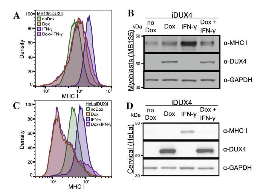
Figure 1. FACS data (A and C) and western blot data (B and D) showing effects of DUX4 activation (via doxycycline) and IFN-γ treatment on MHC I protein expression in an inducible myoblast cell line (MB135-iDUX4) and an inducible cancer cell line (HeLa-iDUX4). (A) FACS data of MHC class I protein levels in myoblast cell line (MB135-iDUX4) showing slight upregulation of MHC I with DUX4 activation. (B) FACS data of MHC class I protein levels in a cancer cell line (HeLa-iDUX4) showing downregulation of MHC I with DUX4 activation (C) Western blot data for MHC class I, DUX4, and GAPDH proteins for myoblast cell line (MB135-iDUX4). (D) Western blot data for MHC class I, DUX4, and GAPDH proteins for cancer cell line (HeLa-iDUX4) Modified from Figure 5 in Chew et al , 2019
Also working in the Tapscott Lab, Spens et al. (2023) similarly investigated DUX4 repression of IFN-γ-stimulated gene induction Performing Quantitative Polymerase Chain Reaction (qPCR) on myoblast cell lines with inducible DUX4, they reported that IFN-γ stimulates an increase
in mRNA levels of CXCL9, an IFN-γ-stimulated gene involved in MHC. CXCL9 expression was reduced, but not eliminated, by DUX4 activation (Figure 2) Using chromatin immunoprecipitation, they also found a decrease in STAT1 binding to promoters of immune-related genes with DUX4 activation. They concluded that DUX4 directly suppresses interferondependent gene expression, leading to a reduction in interferon signaling pathway activity Notably, this study did not look at the effect of DUX4 activation in the absence of IFN-γ treatment.
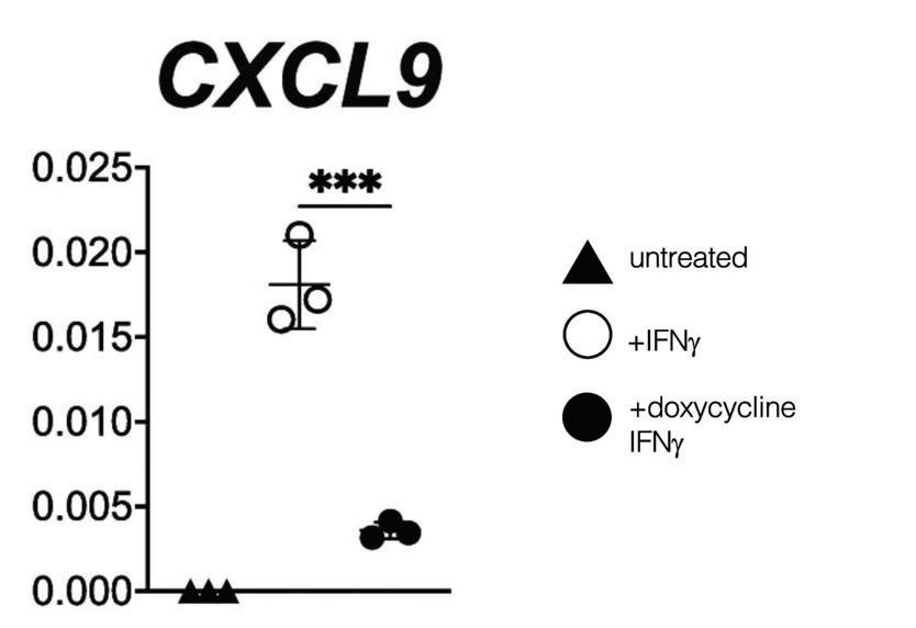
Figure 2. RT-qPCR showing effects of IFN-γ and DUX4 (via doxycycline) treatments on myoblast cell line (MB135-iDUX4) RT-qPCR results of three treatments: untreated, 16 hour IFN-γ, and 4 hour doxycycline followed by 16 hours with IFN-γ in a myoblast cell line (MB135-iDUX4) showing upregulation in the presence of IFN-γ and downregulation in the presence of DUX4 expression (via doxycycline) Modified from Figure 1 in Spens et al , 2023
As part of our duties in the Bosnakovski lab, we ran an experiment designed to test the effects of two drugs on DUX4 induction in the myoblast cell line LHCN-iDUX4 Based on the published results, we looked for decreases in MHC I protein levels as an indicator of DUX4 repressive activity However, using Fluorescence Activated Cell Sorting (FACS) analysis, we found that regardless of DUX4 activation, the samples demonstrated strong, nearly 100%, expression of the MHC I proteins β2-microglobulin (B2M), and human leukocyte antigens (HLA) HLA-A, HLA-B, and HLA-C.
These results conflicted with the data presented by previous research. This research was conducted by a single research group that concluded that DUX4 activation significantly suppresses MHC I expression in all inducible cell lines (Chew et al., 2019). This contradiction between our results and published results led us to wonder whether there may be a difference in how DUX4 behaves in myoblast cell lines versus cancer cell lines, in different versions of inducible DUX4 cell lines, or under different cell culture conditions.
We attempted to replicate published findings of DUX4 suppression of IFN-γ-stimulated MHC class I transcripts and proteins in both myoblast and cancer cell lines using the established protocols and cells used by the Bosnakovski Lab To formally investigate our preliminary observations, we tested whether MHC class I genes in both myoblast and cancer cell lines are suppressed by DUX4 expression in the presence and absence of IFN-γ.
We used six human myoblast cell lines: LHCN-iDUX4, D3F-iDUX4, D13D-iDUX4, 001-56 iDUX4, 007-56 iDUX4, and 008-56 iDUX4 as well as two cancer cell lines: 293T-iDUX4 and A204-iDUX4 All cell lines were DUX4 inducible via doxycycline Only the A 204-iDUX4 cells have been published to demonstrate the downregulation of MHC I with DUX4 induction (Chew et al., 2019). We performed six different treatments on each cell line: a control group treated with cell media; a 16-hour IFN-γ treatment; a 16-hour continuous doxycycline treatment; a 16-hour treatment of IFN-γ and doxycycline; a 4-hour doxycycline pulse followed by 16-hours in cell media; and a 4-hour doxycycline pulse followed by a 16-hour IFN-γ treatment We used FACS analysis to measure protein levels in all cell lines and performed qPCR on one cell line to both confirm that DUX4 was being properly induced and measure MHC class I mRNA levels.
Abigail Getnick and Kelan McKay
Materials and Methods
Cell Culture
Immortalized human myoblast cell lines were cultured according to standard cell culture procedures. Cells were plated in T-25 flasks and transferred to T-75 flasks once they hit 70% confluence Media was changed every three days until cells were confluent enough to plate in 12-well plates filled with 1 mL of the cell solution. The plates were then incubated at 37°C in a 5% CO2 atmosphere until cells had attached to the plate surface and were ready for treatments
Treating Cells
Cells plated in 12-well plates were treated with 10 μM lamivudine (3TC; TargetMol), 10 μM abacavir sulfate (ABC; TargetMol), and 200 ng/mL interferon-gamma (IFN-γ; BioLegend) diluted with cell media DUX4 was induced with doxycycline diluted in cell media to achieve a concentration of 200 ng/mL. The drugs were first added to media in 15 mL tubes to reach their respective dilutions. The well plates were then aspirated and the treatments were added to their respective wells The plates were then incubated at 37°C in a 5% CO2 atmosphere until the treatment period was completed.
Fluorescence Activated Cell Sorting (FACS)
To perform Fluorescence Activated Cell Sorting (FACS) analysis, treated well plates were aspirated and washed with 1x PBS The samples were trypsinized, collected in 15 mL conical tubes, and centrifuged for 5 minutes at 1,300 rpm. The supernatant was aspirated and the samples were washed with 2% FBS PBS. They were then stained with two antibodies, 25 µg/mL HLA-A,B,C (BioLegend) and 100 µg/mL β2-microglobulin (B2M; BioLegend), in a 1:333 dilution with 2% FBS PBS. After staining, the samples were washed with 2% FBS PBS and resuspended in a solution of propidium iodide (MilliporeSigma) The samples were then run using a BD FACSAria flow cytometer Data was analyzed using FlowJo (BD Biosciences)
RNA Extraction
After treatments, well plates designated for RNA analysis were aspirated, washed with 1x PBS, and stored at -80ºC until ready for RNA extraction Standard RNA isolation procedures used to extract RNA with Zymo Research Direct-zol Miniprep Kit RNA samples were then brought to the NanoDrop 2000 spectrophotometer (Thermo Fisher Scientific) to measure their concentrations before storing them at -80ºC for future needs
Quantitative Polymerase Chain Reaction (qPCR)
To perform Quantitative Polymerase Chain Reaction (qPCR), “master mixes” were created for each probe and primer being used For each master mix, 2.2 μl of premix per sample was used. Premix Ex Taq (Probe qPCR, Takara) was used for probes and TB Green Premix Ex Taq II (Primer qPCR, Takara) was used for primers The premix was combined with 0 044 μL of Rox Reference Dye II (Takara) per sample, 0 248 μL of HyPure Molecular Biology Grade Water per sample, and 0.066 μL of the respective probe or primer per sample The master mixes were vortexed thoroughly and spun down before being stored on ice A multichannel pipette was used to plate the master mixes and cDNA samples in triplicates for qPCR in a 384-well plate. Samples were run using a QuantStudio 6 Flex Real-Time PCR System (Applied Biosystems) Data was obtained using the 7500 System Software (Applied Biosystems) For analysis, all probes and primers were normalized to ACTINB, a common housekeeping gene used because of its high expression across many different cells (Chin, 2020)
Results
Confirming DUX4 Activation
To confirm DUX4 activation via doxycycline, qPCR was run on LHCN-iDUX4 cells to measure the expression of DUX4 target genes. When DUX4 is turned on, it activates a set of target genes that can lead to apoptosis, degrade myoblast cells (causing FSHD), and suppress the immune response Because DUX4 is extremely
difficult to identify due to only being detectable in extremely low levels (<0.1% of cells), target genes such as LEUTX and ZSCAN4 are commonly used as biomarkers to indicate DUX4 expression (Banerji et al , 2020) ZSCAN4 mRNA levels were significantly higher (p≤0.01; ANOVA; Figure 3) in all treatments that included doxycycline (the 4 hour doxycycline treatment followed by IFN-γ, the 4 hour doxycycline treatment alone, the 16 hour combination treatment of doxycycline + IFN-γ, and the 16 hour doxycycline treatment alone) compared to the control.
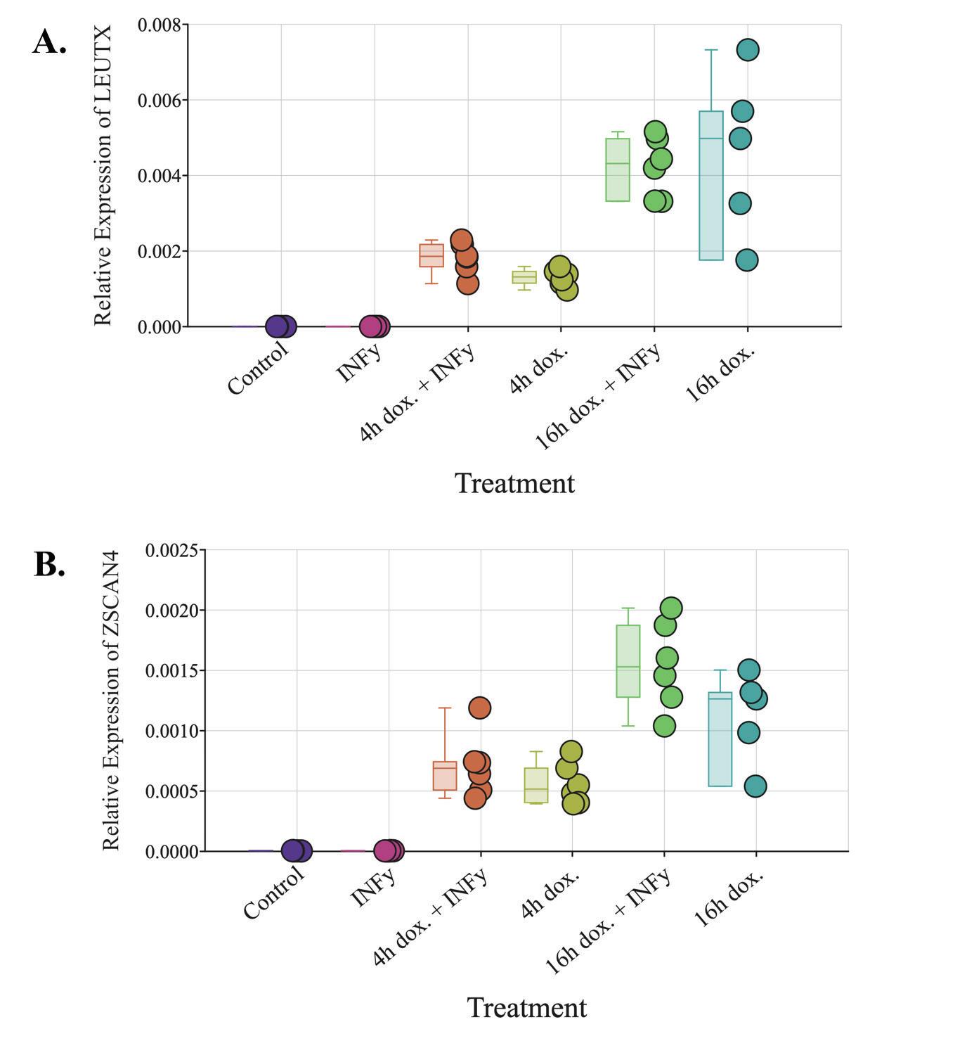
Figure 3. qPCR results for DUX4 target genes on LHCN-iDUX4 cells (A) Relative expression of LEUTX with respect to ACTINB in LHCN-iDUX4 cells (B) Relative expression of ZSCAN4 with respect to ACTINB in LHCN-iDUX4 cells Control: cells cultured in 20% FBS HMM (n=6). IFN-γ: 16 hour treatment with 200 ng/mL IFN-γ (n=6) 4h dox and IFN-γ: 4 hour exposure to 200 ng/mL doxycycline followed by a 16 hour treatment with 200 ng/mL IFN-γ (n=6). 4h dox: 4 hour exposure to 200 ng/mL doxycycline followed by a 16 hour period in 20% FBS HMM (n=6) 16h dox and IFN-γ: 16 hour treatment with 200 ng/mL doxycycline and 200 ng/mL IFN-γ (n=6) 16h dox: 16 hour treatment with 200 ng/mL doxycycline (n=5). (Figure by authors).
Compared to the control, LEUTX mRNA levels were also significantly higher in all samples
treated with doxycycline with the exception of the 4 hour doxycycline treatment. Both LEUTX and ZSCAN4 mRNA levels were significantly higher in the 16 hour doxycycline treatment compared to the 4 hour doxycycline treatment LEUTX and ZSCAN4 mRNA levels were significantly upregulated (p<0.05) in the 4 hour doxycycline + IFN-γ treatment compared to the IFN-γ treatment alone LEUTX and ZSCAN4 mRNA expression also increased significantly (p<0 01) in the 16 hour doxycycline + IFN-γ treatment compared to the IFN-γ treatment alone.
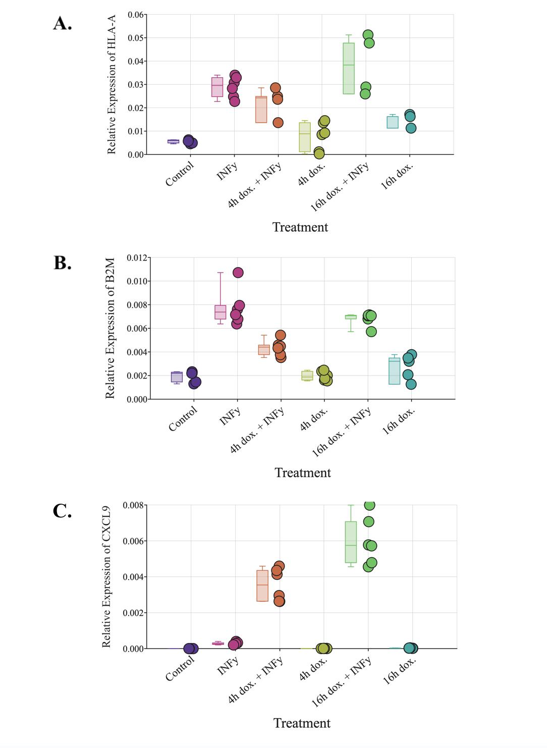
Effect of DUX4 on B2M and HLA-A mRNA expression
The qPCR was also run on LHCN-iDUX4 cells for MHC class I genes HLA-A and B2M. HLA-A is one of the three types of MHC class I genes found in humans that present antigens on a cell ’s surface (Janeway et al , 2001) B2M is also vital to the function of MHC class I (Wang et al., 2021). HLA-A and B2M mRNA levels both significantly increased (p<0.01; ANOVA; Figure 4) in samples treated with IFN-γ compared to the control HLA-A and B2M mRNA levels were also significantly higher (p<0.01) in the 4 hour doxycycline + IFN-γ treatment compared to the control. There was a significant increase (p<0 01) in B2M mRNA in the IFN-γ treatment compared to the 4 hour doxycycline + IFN-γ treatment, but HLA-A mRNA did not show a similar significant increase between these two treatments. The 4 hour doxycycline + IFN-γ treatment also had significantly higher (p<0 05) HLA-A and B2M mRNA levels than the 4 hour doxycycline pulse alone The HLA-A and B2M mRNA levels were not significantly different in the 4 hour doxycycline pulse alone compared to the control. The 16 hour doxycycline + IFN-γ treatment caused significantly higher (p<0 01) HLA-A and B2M mRNA levels compared to the control as well as significantly higher (p<0 05) HLA-A and B2M mRNA levels compared to the 4 hour doxycycline + IFN-γ treatment. The 16 hour doxycycline + IFN-γ treatment did not cause significantly different HLA-A or B2M mRNA levels compared to the treatment of
Abigail Getnick and Kelan McKay
IFN-γ alone but did cause significantly higher levels of HLA-A and B2M mRNA (p<0.01) compared to the 16 hour doxycycline treatment There was no significant change in HLA-A or B2M mRNA levels between the 16 hour doxycycline treatment and the control or between the 4 hour and 16 hour doxycycline treatments.
exposure to 200 ng/mL doxycycline followed by a 16 hour period in 20% FBS HMM (n=6) 16h dox and IFN-γ: 16 hour treatment with 200 ng/mL doxycycline and 200 ng/mL IFN-γ (HLA-A: n=4; B2M: n=6) 16h dox: 16 hour treatment with 200 ng/mL doxycycline (HLA-A: n=3; B2M: n=5) (Figure by authors)
Effect of DUX4 on CXCL9 mRNA expression
CXCL9 is a chemokine that plays a vital role in signaling T cells toward tumor sites and is known to be upregulated by IFN-γ (Ding et al., 2016). Unexpectedly, when compared to the
control, the IFN-γ treatment did not significantly increase the level of CXCL9 mRNA. However, there was a significant increase (p<0 01; ANOVA; Figure 5) in the level of CXCL9 mRNA from the control to the 4 hour doxycycline pulse + IFN-γ treatment. The 16 hour doxycycline + IFN-γ treatment also caused a significant increase in the CXCL9 mRNA level (p<0 01) compared to the control The 16 hour doxycycline + IFN-γ treatment samples had even higher (p<0 01) mRNA levels than the 4 hour doxycycline + IFN-γ treatment. Both the sample treated with 4 hours of doxycycline and the sample treated with 16 hours of doxycycline showed no significant difference in CXCL9 mRNA levels when compared to each other or the control
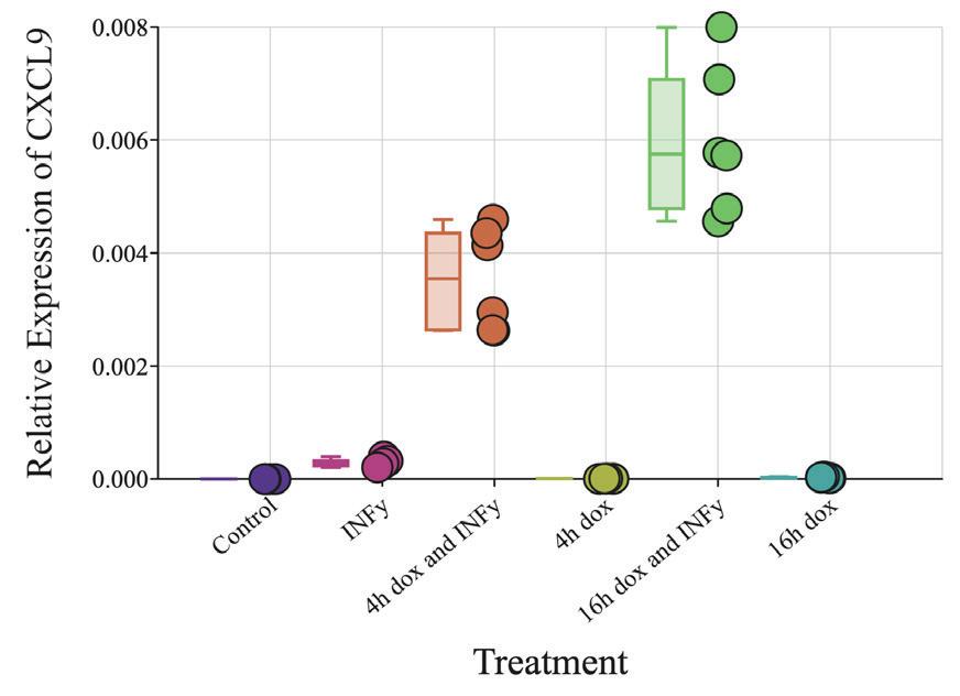
Figure 5. qPCR result for CXCL9 on LHCN-iDUX4 cells. Relative expression of CXCL9 with respect to ACTINB in LHCN-iDUX4 cells.
Control: cells cultured in 20% FBS HMM (n=6) IFN-γ: 16 hour treatment with 200 ng/mL IFN-γ (n=6) 4h dox and IFN-γ: 4 hour exposure to 200 ng/mL doxycycline followed by a 16 hour treatment with 200 ng/mL IFN-γ (n=6) 4h dox: 4 hour exposure to 200 ng/mL doxycycline followed by a 16 hour period in 20% FBS HMM (n=6) 16h dox and IFN-γ: 16 hour treatment with 200 ng/mL doxycycline and 200 ng/mL IFN-γ (n=6). 16h dox: 16 hour treatment with 200 ng/mL doxycycline (n=5) (Figure by authors)
Effect of DUX4 on MHC I protein expression
To analyze the effect of the treatments on MHC class I protein levels, FACS analysis was performed on each cell line. Only minor differences in HLA-ABC levels across treatment groups were observed in LHCN-iDUX4 (Figure
6A) and 293T-iDUX4 (Figure 6B). In LHCN-iDUX4, HLA-ABC proteins were found in 89 7% of the unstimulated (control) cells, 89 6% of the cells treated with IFN-γ alone, 82 6% of the cells treated with the 4-hour doxycycline + IFN-γ treatment, 82.6% of the cells treated with the 4-hour doxycycline pulse, 84.2% of the cells treated with 4-hour doxycycline pulse + IFN-γ treatment, and 84% of the cells treated with both the 16-hour doxycycline treatment as well as the 16 hour doxycycline + IFN-γ treatment.
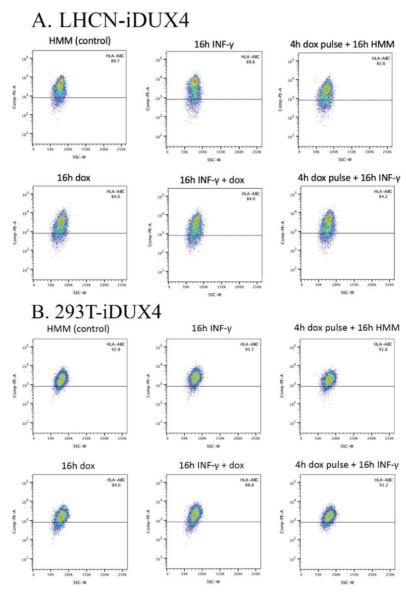
Figure 6. FACS results for HLA-ABC antibody on a myoblast cell line (LHCN-iDUX4) and cancer cell line (293T-iDUX4) showing levels of MHC class I protein expression. (A) FACS results for HLA-ABC antibodies in LHCN-iDUX4 cells (B) FACS results for HLA-ABC antibodies in 293T-iDUX4 cells Control: cells cultured in FBS HMM. IFN-γ: 16 hour treatment with IFN-γ. 4h dox and IFN-γ: 4 hour exposure to doxycycline followed by a 16 hour treatment with IFN-γ 4h dox: 4 hour exposure to doxycycline followed by a 16 hour period FBS HMM 16h dox and IFN-γ: 16 hour treatment with doxycycline and IFN-γ. 16h dox: 16 hour treatment with doxycycline (Figure by authors)
In the 293T-iDUX4 cells, HLA-ABC proteins were present in 92 8% of the unstimulated (control) cells, 95 7% of the cells treated with the 16-hour IFN-γ treatment, 91 8% of the cells treated with the 4-hour doxycycline treatment, 91.2% of the cells treated with the 4-hour doxycycline pulse + IFN-γ treatment, 84% of the cells treated with the 16-hour doxycycline treatment, and 88 8% of the cells treated with the 16-hour IFN-γ + doxycycline treatment
Discussion
Conclusions
Much of the qPCR data gathered contradicts previously reported findings with respect to gene regulation Analysis of LEUTX mRNA confirmed the successful induction of DUX4 However, HLA-A and B2M mRNA analysis demonstrated that DUX4 activation did not consistently downregulate IFN-γ stimulated gene expression, contradicting past research which had found a strong repression effect
As expected, CXCL9 showed significant upregulation in cells treated with IFN-γ, however, this upregulation only occurred in samples also treated with doxycycline Very surprisingly, the samples treated with IFN-γ alone did not demonstrate a significant increase in CXCL9 mRNA levels. Both wells treated with IFN-γ produced this same result, which further points to these interactions being much more complicated in myoblast cells than was previously expected
Contrary to previously published observations, and despite differences we observed in mRNA levels, we did not see a significant difference in MHC class I protein levels regardless of DUX4 induction. Six of our eight cell lines five myoblast lines and one cancer cell line had MHC class I proteins present in close to 100% of cells Only two cell lines one myoblast and one cancer showed any change in HLA-ABC, resembling previously published results that DUX4 induction downregulates MHC I protein levels and IFN-γ upregulates MHC I protein
Abigail Getnick and Kelan McKay
levels. However, these differences were not large enough to be considered significant.
Our FACS results indicate that IFN-γ treatment leads to an increase in the transcription of MHC class I genes, while doxycycline treatments have a repressional effect. However, this does not translate into decreases in protein levels, as was shown in previous research
Limitations and Future Work
Although unlikely, it is possible that the differences between our results and published results may have occurred due to procedural discrepancies between our lab and the other research group’s lab Additionally, differences in doxycycline used may have had an effect on observed results, as our concentration was significantly lower (200ng/mL) than that of previous researchers (1µg/mL). The variable half-lives of MHC I proteins also may have impacted our results, as the cells analyzed could have had residual proteins produced prior to treatment that survived through the treatment period.
Important future steps for analysis include running qPCRs on all cell lines worked with and expanding the diversity of markers used to clarify observed discrepancies. Running a western blot to confirm FACS results would further verify these results Expanding the number of cell lines involved in the experiment, especially to include more cancer cell lines, would also help in confirming observations and solidifying conclusions.
Overall, our results underscore the importance of avoiding assumptions in scientific research and show that it is essential to verify results through repeated experimentation Further research to clarify the relationship between DUX4 activation and MHC I genes and proteins is necessary and could allow researchers to develop new methods of targeting and destroying cancer.
Acknowledgments
We would first like to thank our teacher, Dr. Kragtorp, for all of her assistance throughout the research and writing processes. Our project would not have been possible without her guidance and constant support We would also like to thank our mentor, Dr Bosnakovski of the University of Minnesota Department of Pediatrics, for providing us with the opportunity, training, and resources to conduct research in a professional laboratory, as well as Ana Mitanoska, Usuk Jung, Ajay Ram Vachanaram, and Erik Toso for all of their guidance in the laboratory. Lastly, thank you to our peers, families, and friends for their invaluable feedback and for all of their encouragement in our pursuits of research
References
Banerji, C R S , Panamarova, M , & Zammit, P S (2020) DUX4 expressing immortalized FSHD lymphoblastoid cells express genes elevated in FSHD muscle biopsies, correlating with the early stages of inflammation Human Molecular Genetics, 29(14), 2285 https://doi org/10 1093/hmg/ddaa053
Chew, G -L , Campbell, A E , De Neef, E , Sutliff, N A , Shadle, S C , Tapscott, S J , & Bradley, R K (2019) DUX4 Suppresses MHC Class I to Promote Cancer Immune Evasion and Resistance to Checkpoint Blockade Developmental Cell, 50(5), 658-671 e7
https://doi org/10 1016/j devcel 2019 06 011
Chin, G (2020, November 27) Quantitative Polymerase Chain Reaction Protocol SENS Research Foundation
https://www sens org/quantitative-polymerase-chain-reaction-proto col/
Cornel, A M , Mimpen, I L , & Nierkens, S (2020) MHC Class I Downregulation in Cancer: Underlying Mechanisms and Potential Targets for Cancer Immunotherapy Cancers, 12(7), 1760 https://doi org/10 3390/cancers12071760
Dandapat, A , Bosnakovski, D , Hartweck, L M , Arpke, R W , Baltgalvis, K A , Vang, D , Baik, J , Darabi, R , Perlingeiro, RitaC R , Hamra, F K , Gupta, K , Lowe, D A , & Kyba, M (2014)
Dominant lethal pathologies in male mice engineered to contain an X-linked DUX4 transgene Cell Reports, 8(5), 1484–1496
https://doi org/10 1016/j celrep 2014 07 056
Das, A T , Tenenbaum, L , & Berkhout, B (2016) Tet-On Systems For Doxycycline-inducible Gene Expression. Current Gene Therapy, 16(3), 156–167 https://doi.org/10.2174/1566523216666160524144041
Ding, Q , Lu, P , Xia, Y , Ding, S , Fan, Y , Li, X , Han, P , Liu, J , Tian, D , & Liu, M (2016) CXCL9: Evidence and contradictions for its role in tumor progression Cancer Medicine, 5(11), 3246
https://doi org/10 1002/cam4 934
Janeway, C A , Jr, Travers, P , Walport, M , & Shlomchik, M J
(2001) The major histocompatibility complex and its functions In Immunobiology: The Immune System in Health and Disease 5th edition Garland Science https://www.ncbi.nlm.nih.gov/books/NBK27156/
Karpukhina, A , Tiukacheva, E , Dib, C , & Vassetzky, Y S (2021) Control of DUX4 Expression in Facioscapulohumeral Muscular Dystrophy and Cancer Trends in Molecular Medicine, 27(6), 588–601 https://doi org/10 1016/j molmed 2021 03 008
Pineda, J M B , & Bradley, R K (2023) DUX4 is a common driver of immune evasion and immunotherapy failure in metastatic cancers eLife, 12 https://doi org/10 7554/eLife 89017 1
Prevosto, C , Usmani, M F , McDonald, S , Gumienny, A M , Key, T , Goodman, R S , Gaston, J S H , Deery, M J , & Busch, R (2016) Allele-Independent Turnover of Human Leukocyte Antigen (HLA) Class Ia Molecules PLOS ONE, 11(8), e0161011 https://doi org/10 1371/journal pone 0161011
Schätzl, T , Kaiser, L , & Deigner, H -P (2021)
Facioscapulohumeral muscular dystrophy: Genetics, gene activation and downstream signalling with regard to recent therapeutic approaches: an update Orphanet Journal of Rare Diseases, 16, 129 https://doi org/10 1186/s13023-021-01760-1
Smith, A A , Nip, Y , Bennett, S R , Hamm, D C , Lemmers, R J L F , Van Der Vliet, P J , Setty, M , Van Der Maarel, S M , & Tapscott, S J (2023) DUX4 expression in cancer induces a metastable early embryonic totipotent program Cell Reports, 42(9), 113114 https://doi org/10 1016/j celrep 2023 113114
Spens, A E , Sutliff, N A , Bennett, S R , Campbell, A E , & Tapscott, S J (2023) Human DUX4 and mouse Dux interact with STAT1 and broadly inhibit interferon-stimulated gene induction eLife, 12, e82057 https://doi org/10 7554/eLife 82057
Wang, H , Liu, B , & Wei, J (2021) Beta2-microglobulin(B2M) in cancer immunotherapies: Biological function, resistance and remedy Cancer Letters, 517, 96–104 https://doi org/10 1016/j canlet 2021 06 008
Farewell Forever
Degradation of Pentadecafluorooctanoic Acid Using UV-C Light and T itanium Dioxide
Dawson Miller and Caleb Li
Introduction
Per- and polyfluoroalkyl substances (PFAS) are thermally and chemically stable man-made chemicals characterized by a fluorinated carbon chain (Meegoda et al , 2020) Their carbonfluorine bonds give them useful properties, such as heat and water resistance, contributing to their ubiquity in firefighting foams, non-stick pots and pans, furniture, and other consumer and industrial products (Leung et al , 2023) They are known as ‘forever chemicals’ because their strong carbon-fluorine bonds make them difficult to destroy bonds that also give them their useful properties. (Figure 1; Minnesota Pollution Control Agency, 2024; Yang et al., 2024). As a result, they have found their way into the environment in drinking water, fisheries, landfill leachate, and more and are present in humans.
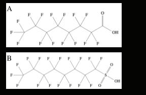
Figure 1. Structure of two long-chain PFAS. (A)
Pentadecafluorooctanoic acid (PFOA) structure (B) Perfluorooctanesulfonic acid (PFOS) structure (Figure generated by authors using chemfig LaTeX package)
Furthermore, these chemicals have serious environmental and health-related concerns like liver tissue damage and hazardous air contamination at concentrations as low as in the parts per trillion (US EPA, 2024a; National Institute of Environmental Health Sciences, n.d.;

Wisconsin DNR, n.d.). The Minnesota based 3M Corporation massproduced and improperly disposed of PFAS, leading to large PFAS plumes contaminating the Minnesota Twin Cities East Metro groundwater and environment (Sharon & Sakaguchi, 2024). While blood PFAS levels have decreased in East Metro residents since 2008, they are still elevated compared to the rest of the United States population (Minnesota Department of Health, n.d.).
PFAS enter the environment through multiple pathways PFAS are first created by factories that discharge their waste into the environment, either through wastewater treatment plants, landfills, or directly to the environment. Airports using aqueous film-forming foam with PFAS for firefighting leach PFAS into surface and groundwater Products containing PFAS from the factories go to consumers and other industries. Ultimately, the general population is exposed to PFAS through consumer goods like food, food packaging, and their city water supply
Because of their ubiquity, persistence, toxicity, and bio-accumulative properties, there is significant interest in researching PFAS containment, removal, and destruction Traditional methods of environmental remediation focus on the removal of contaminants rather than destruction (McIntyre et al , 2022) A few methods for removal are ion exchange, activated carbon, and reverse osmosis Ion exchange filters out target molecules by exchanging them for ions on a rechargeable polymer resin. Activated carbon filters PFAS by adsorption to their porous structure. Reverse osmosis forces water across a semipermeable membrane, rejecting larger molecules like PFAS However, while these methods effectively remove PFAS, they produce concentrated
Dawson Miller and Caleb Li
streams of PFAS that are difficult to destroy effectively (Yadav et al., 2022). Currently, ion exchange resins and granular-activated carbon are typically incinerated, releasing harmful byproducts (McIntyre et al , 2022)
New research has focused on methods to actively destroy PFAS Electrochemical oxidation allows for fast destruction but creates toxic byproducts and requires expensive materials (Yadav et al., 2022). Plasma technology efficiently destroys long-chain PFAS but is less effective with shorter-chain PFAS and requires high energy input Sonochemical technology uses cavitation bubbles from sound to create high temperature, pressure, and chemical radicals that destroy PFAS but performs worse in the presence of inorganic compounds like bicarbonate Although these methods are effective at destroying PFAS, they are limited by specific operating conditions and energy-intensive processes (Yadav et al., 2022).
Another alternative is photocatalysis, which can be performed at room temperature In this method, a photocatalyst is added to a solution containing PFAS. When irradiated with light, the photocatalyst starts different chemical reactions with the potential to break down PFAS Titanium dioxide (TiO2) has been widely researched for its photocatalytic capabilities and has been deployed previously in the destruction of various organic contaminants (Tennakone & Wijayantha, 2005). TiO2 is often used as a reference for testing other photocatalysts and has been regarded as less effective at destroying PFOA compared to photocatalysts like boron nitride (BN), indium oxide (In2O3), and a single-atom platinum SiC photocatalyst (Pt/SiC). Duan et al. (2020) compared the effectiveness of a BN photocatalyst and a P25 TiO2 catalyst in destroying PFOA with 254 nm UV-C light They found that PFOA had a half-life of 1 2 hours for BN compared to 2.4 hours for TiO2. In addition, Li et al. (2012) explored the use of an In2O3 photocatalyst compared to a TiO2 photocatalyst with a 254 nm UV-C light The In2O3 catalyst had a half-life of 1 83 hours for destroying PFOA compared to a 15 40 hour half-life for
TiO2. Hendren et al. (2020) compared Pt/SiC to a TiO2 photocatalyst using a 254 nm UV-C light, which resulted in a half-life of 5 29 hours for Pt/SiC and a half-life of 6 77 hours for TiO2 (Hendren et al , 2020) As shown by its longer half-life for destroying PFOA in these three studies, TiO2 is often less effective at destroying PFOA than other photocatalysts.
PFOA is likely degraded by BN, In2O3, and TiO2 through the decarboxylation, hydroxylation, elimination, and hydrolysis (DHEH) pathway (Figure 2) or a pathway similar to it An electron-hole pair is first created within the photocatalyst when activated with light, allowing oxidation-reduction reactions to occur The carboxyl head of PFOA is first stripped off. Then, a hydroxyl radical formed from water reacting with the electron-hole pair attaches to the carbon chain Hydrogen fluoride is eliminated from the molecule and hydrolysis proceeds, removing one fluorine in the carbon chain and adding a carboxyl head. The cycle is then repeated with the shorter-chain PFAS until the PFOA molecule is completely destroyed (Wong, 2024)
Figure 2. Decarboxylation, hydroxylation, elimination, and hydrolysis (DHEH) pathway (Figure by authors using draw.io with full usage rights).
However, photocatalysts like Pt/SiC use a different reaction pathway The reaction pathway with Pt/SiC first involves removing the carboxyl group from PFOA, followed by hydro-
defluorination a process where fluorine atoms on PFOA are replaced with hydrogen atoms stuck to the catalyst’s surface (Hendren et al , 2020)
TiO2 may be less effective at destroying PFOA than other photocatalysis, but TiO2 is also more readily available than other photocatalysts and inexpensive, so further research on its effectiveness could prove useful (Hendren et al , 2020). TiO2 has been found to be more effective in destroying PFOA at a lower pH (Liang et al., 2023) Hendren et al (2020) used oxalic acid to control the pH of the reaction at 5 We created a system that could destroy PFAS in a high school laboratory using cheap equipment both an inexpensive UV-C light and an inexpensive catalyst. We attempted to optimize the TiO2 photocatalytic system with oxalic acid for pH control and hydrogen peroxide (H2O2) for increased hydroxyl radical production
Materials and Methods
System Design
We designed our system based on Hendren et al. (2020) with modifications to fit our budget and the availability of materials (Figure 3).
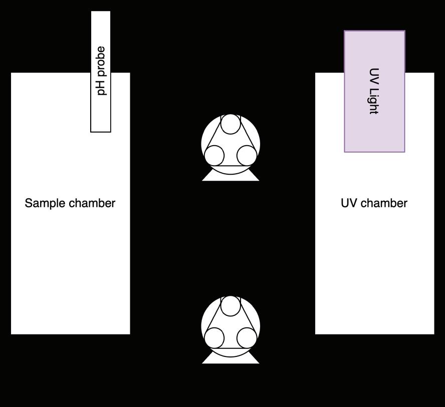
3 Diagram of system (Figure by authors using draw.io with full usage rights).
Two chambers held the solution in the experiment: a sample chamber and a UV-C chamber The sample chamber housed a pH
probe, provided easy access for taking samples during the experiment, and offered us protection from the harmful UV-C light The UV chamber housed the UV-C light, and the reaction took place there Magnetic stirrers ensured proper mixing within each chamber, and two peristaltic pumps moved the solution between the two chambers (Figure 3).
The sample chamber was a 250 mL borosilicate beaker, and the UV chamber was a 500 mL borosilicate graduated cylinder. An 11 W 254 nm UV-C light (Aquarium Clean Light, [11W], JAHEA) was placed inside the graduated cylinder in direct contact with the solution, which was poured into the graduated cylinder The graduated cylinder was covered with aluminum foil to protect us against the UV-C light (Figure 4)
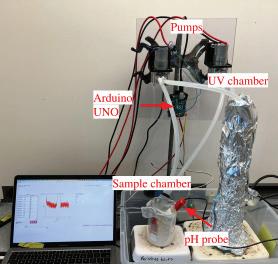
4. Image of the experiment setup UV chamber covered in aluminum foil with the sample chamber center containing the pH probe. Peristaltic pumps mounted above the chambers with tubing extending into both Laptop is running pH probe software. (Figure by authors).
We took 3 mL samples from the sample chamber throughout the experiment to track the reaction progress Each chamber contained a stir bar and was placed on a magnetic stirrer To transfer the solution between the two chambers, we used two stainless steel peristaltic pumps (500 mL/min Large Flow Stainless Steel Peristaltic Pump
Figure
Figure
Dawson Miller and Caleb Li
[12V], Vikye) attached to two separate power supplies; each pump had two silicon tubes (ID 6 35 mm OD 9 54 mm) attached to it Before turning on the UV-C light and the pumps, we covered both the beaker and graduated cylinder in Parafilm “M” Laboratory Film to avoid evaporation.
Water Detection and pH Probe
A water sensor for Arduino (Elegoo Upgraded 37 in 1 Sensor Modules Kit) was used to prevent water from overflowing in either chamber. We altered existing code for an analog water level sensor to program the Arduino and used a 5V relay pinout to turn off one pump either when the water level reached a certain height determined by the water sensor or when the water level continued to rise in the beaker without the water sensor being triggered (LastMinuteEngineers.com, 2019). The goal was for the water level in the graduated cylinder to remain around 200 mL The water sensor was hot glued to the inside of the beaker, with the electrodes facing outward. We used a pH probe to track changes in pH during the experiment to better understand the reaction and effectiveness of pH control The pH probe was programmed and set to take data every 10 seconds throughout the experiment (Atlas Scientific and Vernier)
Creating Solutions
We initially dissolved PFOA (33824, SigmaAldrich) in distilled water (dH2O) to create a 100 mg/L (20x) PFOA solution This was then diluted with dH2O to create the 5 mg/L PFOA used in the experiments. To maintain a pH of around 5, conditions reported to improve the photocatalytic reaction (Hendren et al , 2020), we created a 90 μM oxalic acid (194131, Aldrich) solution A 2 85% w/v H2O2 and 5 mg/L PFOA solution was created by mixing 15 mL of 20x PFOA and 285 mL with 3% H2O2 (3% Hydrogen Peroxide, Walgreens).
Reaction Set Up
At the beginning of each trial, we removed the UV-C light, tubes, and magnetic stir bar from the graduated cylinder and poured 300 mL of the experimental solution into the graduated cylinder The beaker and graduated cylinder
were placed on two separate stir plates; the beaker was hot glued to its stir plate to prevent movement caused by the pumps The setup started with approximately 200 mL of 1x PFOA solution in the graduated cylinder and 100 mL in the beaker. We took an initial 3 mL sample from the beaker using a syringe (3ml Syringes Luer Lock Syringe, LabAider) with a 0.22-micron surfactant free cellulose acetate syringe filter (SF-SFCA-2213-S, Globe Scientific) and dispensed it into a 15 mL conical tube For experiments using TiO2, we turned off the pumps and poured 149 mg TiO2 into the beaker. We then turned the magnetic stirrers and pumps back on for five minutes and took another sample This second sample represented the PFOA concentration after PFOA had adsorbed to TiO2 and the glass of the sample/UV chambers. The pumps and stirrers were turned back on after sampling and the UV-C light and pH probe was turned on Samples were taken as described above at 15 minutes, 30 minutes, 45 minutes, one hour, two hours, three hours, four hours, five hours, and six hours. The samples were stored in a refrigerator set below 6°C (USEPA, 2024) The exact time of each sample collection was recorded After six hours of run ning the system, we turned off one pump to allow all the leftover solution to accumulate in the graduated cylinder for collection. We ran dH2O through the system for 10 minutes to clean the tubes and chambers; this solution was collected in a separate hazardous waste storage container
Some experiments were run for longer than six hours In these cases, at the end of the day, we transferred all of the solution from the two chambers into the UV chamber, letting the reaction run overnight. We took a sample on the morning of the next day, as well as around noon and in the late afternoon (samples were approximately three hours apart); the exact timing of each sample was recorded Longer experiments were run for two or three days
We repeated this procedure with a base solution of 1x oxalic acid and 2 85% H2O2 Each of these experiments was repeated twice to check for
consistency. We also ran one experiment with 1x oxalic acid and 2.82% H2O2 together. Finally, we ran experiments without TiO2 using oxalic acid, hydrogen peroxide, and PFOA only to quantify the effects of using the UV-C light without a photocatalyst in each of these scenarios.
Analytical Methods
We prepared our samples for LC-MS/MS by creating a 1:100 dilution in reverse osmosis water We stoppered and inverted the volumetric flask to mix. Then, we transferred 1 mL of the diluted sample to a glass vial and added 83 μL of extracted internal standard; the vial was capped and mixed by shaking
Analysis was performed with LC-MS/MS composed of high-performance liquid chromatography (HPLC, Agilent 1200 Series) connected to electrospray ionization tandem mass spectrometry in a triple quadrupole mass spectrometer (Sciex API 4000 LC-MS/MS) A Phenomenex C18 column (2.0 x 50 mm, 3.0 μm particle size) with a guard column (2.1 x 55 mm, 5 0 μm particle size) was used for separation The column oven temperature was set to 40°C Samples were eluted with mobile phase composition: (A) 90:10 methanol v/v and (B) methanol; both had 2 mM ammonium acetate. The gradient mode: 100% A at 0 min, 40:60 A:B at 1 5 min, 0:100 A:B at 21 min, and 100% A from 25 to 28 min The flow rate was 200 μL min-1, and the injection volume was 5 μL Peak integration was performed for each sample, and area counts were converted to concentrations using the calibration standard response factor for each analyte (US EPA, 2024b)
Results
We ran four groups of experiments: TiO2, TiO2 with oxalic acid, TiO2 with hydrogen peroxide (H2O2), and a control experiment without any TiO2. The UV-C light was used in all experiments
Three experiments were run with 5 mg/L PFOA, TiO2, and UV-C light. The first yielded a decrease in PFOA concentration of 37 96% in 6 00 hours; the second yielded a decrease of
Dawson Miller and Caleb Li
25.69% in 6.00 hours; the third yielded a decrease of 77.20% in 29.30 hours. We determined the pseudo-first-order rate constant to be about 1 41 day-1 and the half-life to be about 11 8 hr-1 (Figure 5) The average pH between the first and second runs was 3.84; pH data for the third run was inaccurate due to improper calibration.
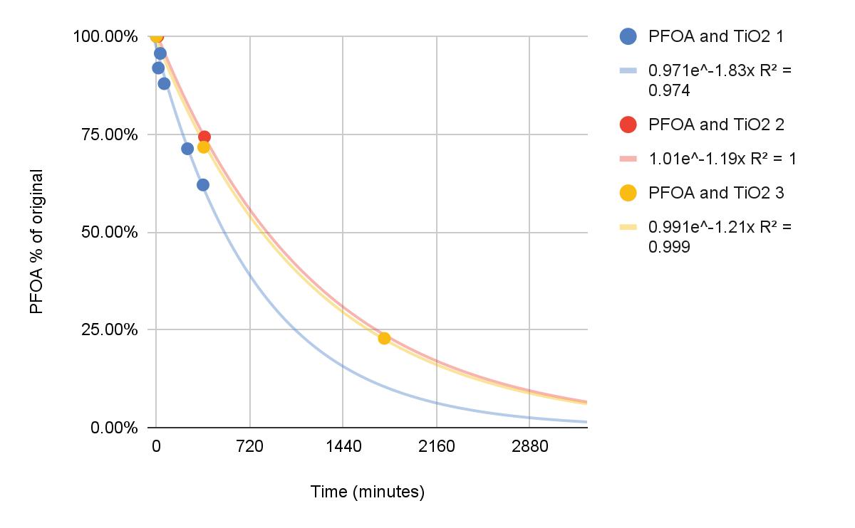
Figure 5. PFOA destruction over time (percent of original concentration), with TiO2 (Figure by authors)
One experiment with 5 mg/L PFOA, TiO2, oxalic acid, and UV-C light yielded a decrease in PFOA concentration of 66.89% in 29.55 hours. The second experiment with the same variables yielded a decrease in PFOA concentration of 78 60% in 29 92 hours We determined the pseudo-first-order rate constant to be about 1 09 day-1 and the half-life to be about 15 3 hr (Figure 6). The average pH, using data collected from both runs, was 3.86.
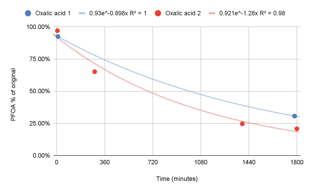
Figure 6. PFOA destruction over time (percent of original concentration) with oxalic acid and TiO2 (Figure by authors).
Two experiments were run with 5 mg/L PFOA, TiO2, hydrogen peroxide, and UV-C light; one
for 29.98 hours and the other for 46.97 hours. There was no detectable decrease in PFOA concentration throughout the experiment (Figure 7) The average pH, using data from both runs, was 7 68
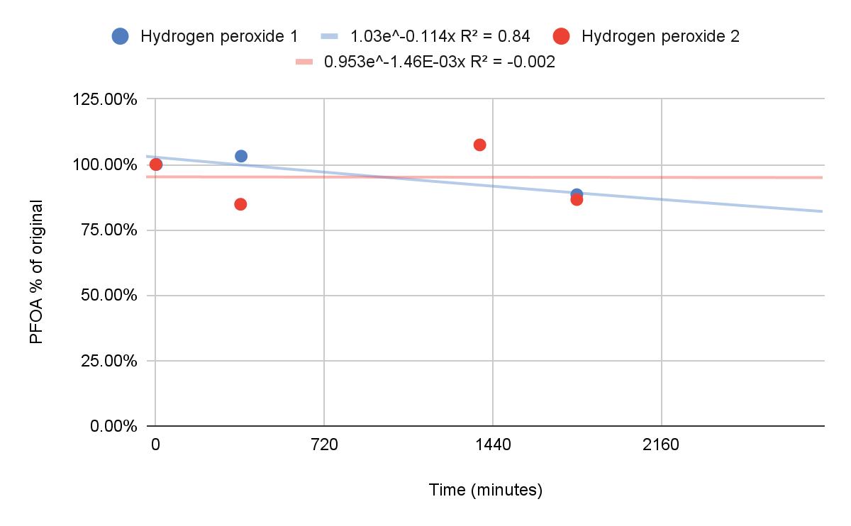
Figure 7. PFOA destruction over time (percent of original concentration) with hydrogen peroxide and TiO2 (Figure by authors)
One experiment was run with only 5 mg/L PFOA and UV-C light. This resulted in a decrease in PFOA concentration of 97 40% in 44 38 hours with a half-life of 11 2 hr-1 Another experiment was run with 5 mg/L PFOA, UV-C light, and oxalic acid. This resulted in a decrease in PFOA concentration of 97.77% in 61.52 hours with a half-life of 8.44 hr-1 (Figure 8). The pH was not measured during this experiment
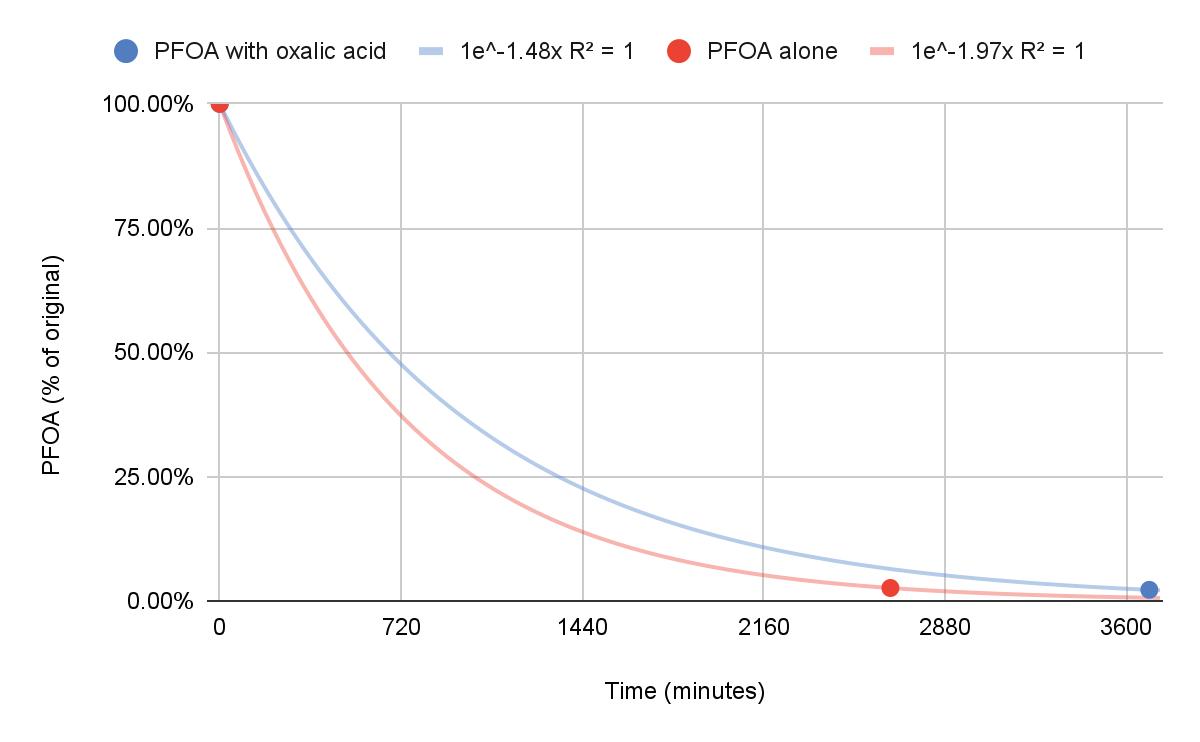
Figure 8. PFOA destruction over time (percent of original concentration) using only UV-C light, with and without oxalic acid (Figure by authors)
Further analysis revealed shorter-chain PFAS in samples for UV-C light with TiO2, UV-C light alone, and UV-C light with TiO2 and oxalic acid
Discussion
The TiO2 and UV-C light successfully destroyed PFOA. In 6 hours, about 32% of PFOA was broken down. In 29 hours, about 77% of PFOA was broken down The oxalic acid in conjunction with TiO2 and UV-C light did not yield additional destruction compared to TiO2 and UV-C light. The pH of the experimental solution with oxalic acid remained at about 3.8, which was the same as the TiO2 and UV-C light experiment without oxalic acid The lack of difference in pH could explain the absence of additional PFOA destruction The hydrogen peroxide with TiO2 and UV-C light appeared to inhibit the reaction since there was no measurable destruction of PFOA when hydrogen peroxide was present This may be due to preservatives like sodium citrate in our hydrogen peroxide that interfered with the production and effectiveness of hydroxyl radicals for degrading PFOA; in addition, we do not know if the hydrogen peroxide had decomposed by the time we were using it The pH of the experiments with hydrogen peroxide was higher than the oxalic acid and TiO2 experiments, with a pH of about 6.8 this is also a possible explanation for the inhibition of the reaction because the reaction with TiO2 works best at a lower pH
The most surprising result from these trials was that the UV-C light alone, which we had initially intended as a control for the other trials, appears to destroy PFOA the fastest out of all the experiments we ran, with a pseudo-first-order rate constant of 1.97 day-1. This result contradicts previous research, where TiO2 consistently yields higher destruction rates than direct photolysis (Meegoda et al , 2020) However, the rate constant for the experiment with UV-C light alone is within 10% of the fastest TiO2 and PFOA result we recorded. This is well within the margin of error for the measurements; the hydrogen peroxide measurements, where no PFOA was destroyed, varied by as much as 15% at times In addition, the experiment with UV-C light alone was allowed to run for much longer than the experiments with TiO 2 (61 hours v. 29 hours). The solution in the UV-C light alone experiment
was also in contact with the UV-C light for most of the experiments, rather than being cycled through the pump system PFAS is broken down by direct photolysis when photons of wavelength less than 300 nm directly strike the PFAS molecules, starting photodegradation; it has been known to work faster with 185 nm light, rather than the 254 nm light we used, but those experiments did not immerse the UV-C light in the solution (Verma et al , 2024) Residual TiO2 in the system that stuck to the tubing and UV-C light may have contributed to this result, but this is unlikely to have produced such a significant change in the amount of PFOA destroyed.
Limitations and Future Work
Although we can safely state that the UV-C light and UV-C light with TiO2 effectively destroyed some PFOA, analysis of the samples revealed shorter-chain PFAS in the solution. We do not know if these PFAS are contaminants from our solutions used or if they are PFAS formed due to the stepwise nature of the photocatalytic process More samples, longer reaction times, and analysis for total PFAS concentration would allow us to better understand the nature of the reaction over time.
We also do not know why the oxalic acid solution was ineffective. It was discovered that there were unknown solid substances floating inside the solution we created, suggesting the oxalic acid solution may have had other compounds besides oxalic acid and water this could have potentially inhibited its effectiveness as a pH controller. Our pH probe was not working properly for many of the experiments, limiting the data on whether the oxalic acid controlled pH Using pure oxalic acid with an accurate pH probe would provide information on the efficacy of oxalic acid to improve photocatalysis. The hydrogen peroxide that we used was already opened (so it may have decomposed) We also had not tested the hydrogen peroxide solution beforehand to determine its components unknown compounds or preservatives in the solution could have hindered the degradation of PFOA by blocking the reaction mechanism. In addition,
Dawson Miller and Caleb Li
the sodium citrate used to stabilize the peroxide could have also interfered with the reaction. Fresh hydrogen peroxide, without preservatives, would lend insight into the true effectiveness of hydrogen peroxide on photocatalysis
We also noticed the TiO2 sticking to the sides of the tubing and the UV-C light, which may have changed the concentration of TiO2 within our system As a result, we are unsure whether the concentration of TiO2 was the same between experiments. Additionally, because varying lengths of the experimental runs and pump malfunctions, it is difficult to compare the different conditions Repeating the experiments with quartz glass, which UV-C light can pass through, would allow us to avoid using the pumps entirely, preventing TiO2 from sticking to the tubing and ensuring a constant reaction rate Testing other reaction mediums like lake water or tap water could be used to determine the efficacy of photocatalysis with a diverse range of co-contaminants, ions, and other particles, as well as with other PFAS chemicals.
Implications
Our goal was to create an inexpensive method to destroy PFOA using UV-C light and TiO2 but we were surprisingly successful in destroying PFOA with just the UV-C light. If further analysis confirms the full destruction of the PFOA molecules, our research raises the intriguing possibility that PFOA could be destroyed by individuals on a small scale using UV-C light alone. An individual could collect their water in a container, insert an inexpensive UV-C light for a few days, and be reasonably confident that the majority of the PFOA has been removed all without the hassle of removing or filtering a photocatalyst
Acknowledgments
Dr. Kati Kragtorp and Dr. Brian Trussell helped edit this paper and advised us throughout the project Dr Matt Simcik and Elli Galloway at the University of Minnesota allowed us to analyze our samples
References
Duan, L , Wang, B , Heck, K , Guo, S , Clark, C A , Arredondo, J , Wang, M , Senftle, T P , Westerhoff, P , Wen, X , Song, Y , & Wong, M S (2020) Efficient Photocatalytic PFOA Degradation over Boron Nitride Environmental Science & Technology Letters, 7(8), 613–619 https://doi org/10 1021/acs estlett 0c00434
Hendren, Z , Kim Dong, G , & Kim, J (2020, June 5) Effective destruction of PFAS in water by modified SiC-based photocatalysts (ER18-1513) (ER18-1513) Research Triangle Institute Retrieved May 13, 2024, from https://serdp-estcp-storage s3 us-gov-west-1 amazonaws com/s3fspublic/project documents/ER18-1513 Final Report pdf
LastMinuteEngineers com (2019, November 29) In-Depth: How Water Level Sensor Works and Interface it with Arduino Last Minute Engineers https://lastminuteengineers com/water-level-sensor-arduino-tutorial
Leung, S C E , Wanninayake, D , Chen, D , Nguyen, N -T , & Li, Q (2023) Physicochemical properties and interactions of perfluoroalkyl substances (PFAS) - challenges and opportunities in sensing and remediation Science of The Total Environment, 905, 166764. https://doi.org/10.1016/j.scitotenv.2023.166764
Liang, J , Guo, L , Xiang, B , Wang, X , Tang, J , & Liu, Y (2023) Research Updates on the Mechanism and Influencing Factors of the Photocatalytic Degradation of Perfluorooctanoic Acid (PFOA) in Water Environments. Molecules, 28(11), Article 11. https://doi org/10 3390/molecules28114489
Li, X., Zhang, P., Jin, L., Shao, T., Li, Z., & Cao, J. (2012). Efficient photocatalytic decomposition of perfluorooctanoic acid by indium oxide and its mechanism [Publisher: American Chemical Society] Environmental Science & Technology, 46 (10), 5528–5534 https://doi org/10 1021/es204279u
McIntyre, H , Minda, V , Hawley, E , Deeb, R , & Hart, M (2022)
Coupled photocatalytic alkaline media as a destructive technology for per- and polyfluoroalkyl substances in aqueous film-forming foam impacted stormwater Chemosphere, 291, 132790 https://doi org/10 1016/j chemosphere 2021 132790
Meegoda, J N , Kewalramani, J A , Li, B , & Marsh, R W (2020) A review of the applications, environmental release, and remediation technologies of per- and polyfluoroalkyl substances
[Number: 21 Publisher: Multidisciplinary Digital Publishing Institute] International Journal of Environmental Research and Public Health, 17 (21), 8117 https://doi org/10 3390/ijerph17218117
Minnesota Department of Health (n d ) PFAS biomonitoring in the east metro Retrieved September 6, 2024, from https://www health state mn us/communities/environment/biomonit oring/projects/pfas html
Minnesota Pollution Control Agency (2024, May 20) MPCA brings cutting-edge technology to minnesota to remove PFAS from water Retrieved May 22, 2024, from https://www pca state mn us/news-and-stories/mpca-brings-cuttingedge-technology-to-minnesota-to-remove-pfas-from-water
National Institute of Environmental Health Sciences (n d ) Perfluoroalkyl and polyfluoroalkyl substances (PFAS) [National
institute of environmental health sciences] Retrieved May 20, 2024, from https://www niehs nih gov/health/topics/agents/pfc
Sharon, L , & Sakaguchi, H (2024, May 20) How 3m executives convinced a scientist the forever chemicals she found in human blood were safe [ProPublica] Retrieved June 3, 2024, from https://www propublica org/article/3m-forever-chemicals-pfas-pfos -inside-story
Tennakone, K , & Wijayantha, K G U (2005) Photocatalysis of CFC degradation by titanium dioxide Applied Catalysis B: Environmental, 57 (1), 9–12 https://doi org/10 1016/j apcatb 2004 10 004
US EPA (2024, May 8) Designation of Perfluorooctanoic Acid (PFOA) and Perfluorooctanesulfonic Acid (PFOS) as CERCLA Hazardous Substances
US EPA (2024) Method 1633 analysis of per- and polyfluoroalkyl substances (PFAS) in aqueous, solid, biosolids, and tissue samples by LC-MS/MS
Verma, S , Mezgebe, B , Hejase, C A , Sahle-Demessie, E , & Nadagouda, M N (2024) Photodegradation and photocatalysis of per- and polyfluoroalkyl substances (PFAS): A review of recent progress Next Materials, 2, 100077 https://doi org/10 1016/j nxmate 2023 100077
Wisconsin DNR (n d ) Environmental and health impacts of PFAS Retrieved May 22, 2024, from https://dnr wisconsin gov/topic/PFAS/Impacts html
Wong, M S (2024, May 6) Chemical-Free Light-Driven Destruction of PFAS Using Non-Toxic Boron Nitride [Webinar] https://www youtube com/watch?v=GyBqBzuplxw
Yadav, S , Ibrar, I , Al-Juboori, R A , Singh, L , Ganbat, N , Kazwini, T , Karbassiyazdi, E , Samal, A K , Subbiah, S , & Altaee, A (2022) Updated review on emerging technologies for PFAS contaminated water treatment Chemical Engineering Research and Design, 182, 667–700 https://doi org/10 1016/j cherd 2022 04 009
Yang, H , Park, S -J , & Lee, C -G (2024) Enhanced removal of perfluoroalkyl substances using MMO-TiO2 visible light photocatalyst Alexandria Engineering Journal, 87, 31–38 https://doi org/10 1016/j aej 2023 12 008
The Piece W ithin: Using Matrix Metalloproteinases to Cleave CD200 to Combat Cancer
Veda Rao and Maria Rohlfsen
Introduction
Cancer is the accumulation of mutated cells that continuously grow and proliferate. Approximately 40% of men and women will be diagnosed with cancer at least one point in their lives (Cancer Statistics, n d ) Tumors are tissues that can potentially have cancerous cells Tumors have the ability to metastasize, meaning they spread to other parts of the body. There are two types of tumors, solid and non-solid (What Is Cancer?, n d ) The patient’s stage and type of cancer influences possible treatment options Cancer stems from a patient’s cells, therefore, most treatments affect the patient’s healthy and cancerous cells, causing negative side effects. For example, chemotherapy is a drug targeted at killing growing cells (Chemotherapy - Mayo Clinic, n d ) Because chemotherapy can also attack normal cells, it can have harmful side effects. Another approach to cancer is radiation. Radiation uses beams of energy to kill cancerous cells Radiation works by destroying the genetic material used by cells to continue to proliferate Similarly to chemotherapy, radiation can also kill the body’s healthy cells (Hall et al., 2022).
Immunotherapy is an alternative approach to cancer treatment that utilizes a patient’s own immune system to clear precancerous or early cancerous cells. One type of immunotherapy is cancer vaccines, which function by training the immune system to better recognize tumor associated antigens, and therefore find and kill cancer cells (Cancer Treatment VaccinesImmunotherapy - NCI, 2019). Vaccines are most successful in early stage cancers but their effectiveness is hindered when cancerous cells activate immune checkpoints to force the immune system into stopping its response (Kaczmarek et al , 2023) CD200 is a protein involved in T cell signaling that regulates T cell activation (Liu et al., 2020). T cells combat

cancer by recognizing the cancerous cells as foreign cells; once they find the cancer, they attack and kill it. Once the cancer has been killed, regulating checkpoints, such as CD200, signal T cells to stop fighting in order to protect healthy cells (Using Your Own Immune System to Fight Cancer | Stony Brook Cancer Center, n.d.). CD200 is also found in tumor lysate from patients undergoing vaccination immunotherapy. When it binds to the CD200 receptor (CD200R), it suppresses the immune response CD200R is found on cells involved in the immune response, such as myeloid cells, leukocytes, or T cells (Rajaram et al., 2014). In addition to CD200R, there is another receptor, CD200 Activation-Receptor (CD200AR) involved in the CD200 pathway Synthetic ligand binding to CD200AR blocks CD200/CD200R activation, restoring the anti-tumor activity of macrophages (Xiong et al., 2020). However, CD200 cannot directly bind to CD200AR, and the natural ligand to CD200AR is not yet known (Moertel et al , 2022)
CD200AR-L is a synthetic peptide based on a portion of the CD200 protein which was created to bind to CD200AR, in order to activate the immune system (Xiong et al , 2020) The peptide was created through analysis of the amino acid sequences of CD200 and CD200AR. Xiong et al. treated murine macrophages containing CD200 with the synthetic CD200AR-L peptide and found that mRNA expression of cytokines was increased, indicating an activation of these cells (Xiong et al., 2020). Re-configured CD200AR-L resulted in increased effectiveness of immunotherapy against breast cancers (Ampudia-Mesias et al , 2021), and likewise, companion dogs with high grade gliomas treated with CD200AR-L overcame the immuno-suppressive effects of
Veda Rao and Maria Rohlfsen
CD200, demonstrating clinical efficacy (Xiong et al., 2020). The NF-κB signaling pathway is an inflammatory pathway involved in the expression of cytokine, chemokines, and other inflammatory proteins (Lawrence, 2009) In cancerous cells, NF-κB leads to tumor cell proliferation, and it suppresses apoptosis. Suppression of the NF-κB pathway in cancerous cells is beneficial, as cancerous cells will then proliferate less and more apoptosis of cancer cells will occur Preliminary research indicates that this pathway is stimulated by endogenous CD200, but blocked by synthetic CD200 fused with the immunoglobulin G1 Fc segment (M Saxena, unpublished observations)
We hypothesized that a peptide derived from cleaved CD200 might be more effective than the synthetic CD200AR-L (Wong et al , 2016) To test this hypothesis, we combined CD200Fc with Matrix Metalloproteinases (MMPs), which are protein enzymes that can break down proteins in the Extracellular Matrix (ECM; Almutairi et al., 2013). When combined with CD200, the MMPs will break down the CD200, potentially producing fragments that can block the binding of CD200 and CD200R or activate CD200AR We used these treatments in vitro on a monocytic cancer cell line derived from mice. Because CD200 stimulates the NF-κB pathway, we used NF-κB expression, as assessed by western blots, as a marker to measure CD200R activation (Nip et al , 2023)
Materials and Methods
Cell Culturing
We moved the cells from the flask to petri dishes, removed the old RPMI media, and added 2 mL of 0 05% Trypsin We put the flask into a 37℃ incubator for 5-15 minutes until the cells were “floating ” Then we added 18 mL of RPMI media to neutralize the trypsin. We centrifuged the cells and RPMI media at 2000 RPM for 2 minutes, removed the trypsin/media, added 10 mL of PBS, then vortexed We centrifuged the cells again at 2000 RPM for 2 minutes, removed the PBS and vortexed the remaining PBS and cells. We added 3 mL of the RPMI media to 22
petri dishes and seeded 3 million cells (75 μl) in each petri dish.
Proliferation Assay
A proliferation assay was completed prior to treatment to ensure that the cells were normal and healthy We plated 1 million cells in two 6-well plates. There were three wells for each of the following timepoints: 18, 24, 48, and 72 hours At each of these timepoints, we took five pictures of the cells using Invitrogen’s EVOS M7000 Imaging System of the three wells At each time point, five images were taken of each well using Invitrogen’s EVOS M7000 Imaging System. Cell counts were calculated using Image J We created 1:10 and 1:5 dilutions of the cells and added 10 μl of trypan blue We used the Invitrogen’s Countess automated cell counter to determine the number of cells in each sample.
Treatments
Cells were treated in batches of three petri dishes with one of the following treatments (Table 1): MMP-2 (16nM) with or without CD200Fc, MMP-3 (16nM) with or without CD200Fc, MMP-9 (16nM) with or without CD200Fc, and all 3 MMPS with CD200Fc. In ad dition, CD200Fc was used alone Saline was used as a control
Table 1. Summary of the combinations of CD200Fc and Matrix Metalloproteinase added to cells
CD200Fc (10 μg/mL)
MMP-2 (16 nM)
MMP-3 (16 nM)
MMP-9 (16 nM)
We removed the old media and replaced it with new media containing the treatments Cells were
incubated with the treatments at room temperature for five minutes. Then we removed the media and treatment mixture and scraped the cells We rinsed the petri dish with 2 mL of 1x PBS then spun this down at 2000 RPM for two minutes. Cells were stored at -80 ℃ .
Western Blots
We created cell lysates to analyze the cells using western blots Cells were removed from -80 ℃ and thawed on ice We then added 180 μl of cell lysis buffer (RIPA and extraction buffer from Thermo Scientific) and 10 μl of protease inhibitor cocktail, depending on the amount of cells present, then incubated for 30 minutes on ice before centrifuging tat 16000 RPM at 4 ℃ for 10 minutes
We performed a BCA assay following the Thermo Scientific Pierce BCA protein assay kit protocol to determine the volume of lysate necessary for there to be 20 μg of protein in each well. We added 6 μl of the 6x loading dye and brought the volume to 25 μL with 1x RIPA buffer (ThermoScientific) We heated the samples using a Dri-Bath at 100 ℃ for 6 minutes, then cooled them to 37 ℃ and spun at 1500 RPM for 2 minutes. We poured a 1x running buffer into the electrophoresis apparatus (Bio Rad). We loaded 10 μl of the marker and up to 42 μl of our samples We ran the gel at 120 V for about 1 hour or until the dye passed the bottom of the gel
We transferred the protein on the gel to the polyvinylidene fluoride membrane We cut six pieces of filter paper to fit the size of the gel We then soaked the fiber sponge and filter paper in a 1x transfer buffer and wet the membrane in methanol. We removed the gel from the plastic plates then assembled the “sandwich” with the black side of the gel holder cassette on the bottom, then the fiber sponge, two pieces of filter paper, the gel, the membrane, two more pieces of filter paper, another fiber sponge, and then the white side of the gel cassette holder. We made sure that there were no air bubbles between the gel and membrane We put the sandwich into the electroporator with ice packs to ensure the temperature did not rise. We
Veda Rao and Maria Rohlfsen
covered the sandwich with a transfer buffer. The membrane was in between the gel and the positive side We then transferred this at 120 V for 50 minutes We carefully removed the membrane from the sandwich We blocked the membrane in 3% Bovine Serum Albumin (BSA) in Tris-Buffered Saline Tween-20 (TBST) for 1 hour. Then we added the NF-κB primary antibody (1:1000; Cell Signaling Technology) The membrane incubated in the BSA and primary antibody overnight at 4 ℃ on a shaker The next day, we brought the blots to room temperature on a shaker. We washed the membrane with TBST for 5 minutes on the shaker We repeated the wash three times Then we added an anti-rabbit horseradish peroxidaselinked secondary antibody (1:1000; Cell Signaling Technology) in 3% BSA in TBST and incubated it for 1.5 hours. We then washed the membrane with TBST three more times. Then, the ECL mixture was created by following the protocol from Thermo Fisher’s Pierce ECL Western Blotting Substrate We covered the membrane in the ECL mixture, while ensuring that no light hits the membrane. We visualized the result using iBright FL1000
Results and Discussion
Cell Proliferation Assay
Cell counts were assessed at 12, 24, 48, and 72 hours prior to treatment to ensure cells were healthy prior to treatment. Average cell counts increased over time (Figure 1). The cells also became more adherent over time (data not shown)
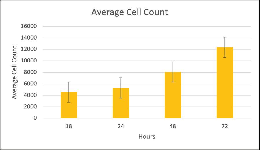
Figure 1. Average cell counts at each time point Cell counts found using Image J (Figure by authors).
BCA Assay
A BCA assay was performed to determine the concentration of protein in each sample after harvesting (Table 2). Concentrations were used to determine how much cell lysate was needed for the western blot
Table 2. Concentration of protein in cells after treatment and amount of cell lysate used in western blot
Treatment Group
CD200Fc + MMP2 2 58 7 76
CD200Fc + MMP3 3 60 5 56
CD200Fc + MMP9 2 49 8 00
CD200Fc + MMP2 + MMP3 + MMP9 2.60 7.68
CD200Fc 2 27 8 80 Saline 3 99 5 02
MMP2 2.00 10.0
MMP3 2 27 8 8
MMP9 2 28 8 76
Western Blot for NFкB
A western blot for NFкB was conducted with cell lysates from all treatments (Figure 2)
β-Actin was used to normalize NF-κB levels, then NF-κB levels for each treatment were compared to the NF-κB level for saline All treatments reduced the expression of NF-κB as compared to saline (Table 3) The MMP3 treatment resulted in the largest decrease in NF-κB levels from saline (0.22), both MMP2 alone and MMP2 in combination with CD200Fc (0 24) had the second largest decrease in NF-κB expression from saline, and MMP3 in combination with CD200Fc had the third largest decrease (0.28).
Table 3. NF-κB fold change from saline treatment
Saline 1 00
CD200Fc 0 40 MMP-2 0 24 MMP-3 0.22
MMP-9 0 48
CD200Fc+MMP2 0 24
CD200Fc+MMP3 0.28
CD200Fc+MMP9 0 40
CD200Fc+MMP2, MMP3, MMP9 0 48
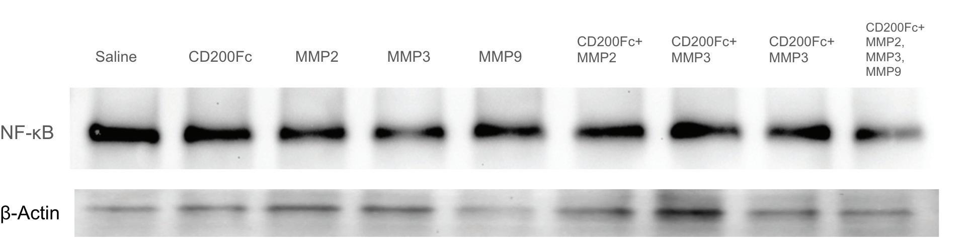
Figure 2. Western Blot for NF-κB and β-Actin
Veda Rao and Maria Rohlfsen
Discussion
All treatments were successful in lowering NF-κB expression, indicating that CD200/ CD200R signaling was inhibited. MMP2 and MMP3 treatments either alone or in combination with CD200Fc were the most successful in creating the correct fragment for blocking the CD200/CD200R interactions that cause immune suppression. The cells likely expressed endogenous CD200, which could have been cleaved by the MMP treatments This cleavage could have been enough to decrease the CD200 signaling This could explain the consistent fold changes for the different MMPs alone and in combination with CD200Fc. However, we cannot discount the possibility that the MMP treatments could be affecting NFkB levels by impacting a pathway other than CD200 signaling.
Limitations and Future Work
Our experiment was a preliminary exploration of the hypothesis that MMPs may create fragments capable of blocking the signaling of CD200/ CD200R We successfully identified likely combinations of MMPs that may create the natural ligand. However, we only did one plate of each treatment and only ran one sample for each treatment on the western blot Future experiments will need to use multiple samples run in the same western blot to ensure the results are replicated and consistent. Additionally, NF-κB is just one indicator of CD200/CD200R signaling, and can be impacted by a variety of other signaling pathways, so there is a need to investigate other pathways of CD200/CD200R signaling and activation to determine whether these results are specific to CD200. Aspects of CD200 activation must also be investigated in other cell types to verify the effectiveness of our treatments in a broader context
All of the treatments reduced NF-κB levels, but some worked better than others. An analysis of the fragments produced by MMPs and CD200Fc will likely help us identify the difference between the fragments produced by MMP2, MMP3, and MMP9. Further research can focus
on determining which fragments interfere with CD200/CD200R or activate CD200AR. Determining the specific ligand could lead to future improvements in cancer vaccines and immunotherapy Blocking the CD200/CD200AR or activating CD200AR are two ways to increase macrophage response against cancerous cells, leading to more effective immunotherapy approaches
Acknowledgments
We would like to thank Dr Michael Olin and Dr. Meghna Saxena from the University of Minnesota’s Masonic Cancer Center for all of their support in our work. We would also like to acknowledge Dr Kati Kragtorp for her guidance
References
Almutairi, S , Kalloush, H M , Manoon, N A , & Bardaweel, S K (2023) Matrix Metalloproteinases Inhibitors in Cancer Treatment: An Updated Review (2013-2023) Molecules (Basel, Switzerland), 28(14), 5567 https://doi org/10 3390/molecules28145567
Ampudia-Mesias, E , Puerta-Martinez, F , Bridges, M , Zellmer, D , Janeiro, A , Strokes, M , Sham, Y Y , Taher, A , Castro, M G , Moertel, C L , Pluhar, G E , & Olin, M R (2021) CD200 Immune-Checkpoint Peptide Elicits an Anti-glioma Response Through the DAP10 Signaling Pathway Neurotherapeutics: The Journal of the American Society for Experimental NeuroTherapeutics, 18(3), 1980–1994 https://doi org/10 1007/s13311-021-01038-1
Cancer Statistics (n d ) https://www cancer gov/about-cancer/understanding/statistics
Cancer Treatment Vaccines Immunotherapy NCI (nciglobal,ncienterprise) (2019, September 24) [cgvArticle] https://www cancer gov/about-cancer/treatment/types/immunothera py/cancer-treatment-vaccines
Chemotherapy Mayo Clinic (n d ) Retrieved June 3, 2024, from https://www mayoclinic org/tests-procedures/chemotherapy/about/ pac-20385033
Hall, W A , Paulson, E , Li, X A , Erickson, B , Schultz, C , Tree, A , Awan, M , Low, D A , McDonald, B A , Salzillo, T , Glide‐ Hurst, C K , Kishan, A U , & Fuller, C D (2022) Magnetic resonance linear accelerator technology and adaptive radiation therapy: An overview for clinicians CA: A Cancer Journal for Clinicians, 72(1), 34–56 https://doi org/10 3322/caac 21707
Kaczmarek, M , Poznańska, J , Fechner, F , Michalska, N , Paszkowska, S , Napierała, A , & Mackiewicz, A (2023) Cancer
Vaccine Therapeutics: Limitations and Effectiveness A Literature Review Cells, 12(17), 2159 https://doi org/10 3390/cells12172159
Le, C , Hao, X , Li, J , Zhong, J , Lin, H , Zhou, Y , Travis, Z D , Tong, L , & Gao, F (2019) CD200Fc Improves Neurological Function by Protecting the Blood–brain Barrier after Intracerebral Hemorrhage Cell Transplantation, 28(9–10), 1321 https://doi org/10 1177/0963689719857655
Liu, J -Q , Hu, A , Zhu, J , Yu, J , Talebian, F , & Bai, X -F (2020) CD200-CD200R pathway in the regulation of tumor immune microenvironment and immunotherapy Advances in Experimental Medicine and Biology, 1223, 155–165 https://doi org/10 1007/978-3-030-35582-1 8
Moertel, C , Martinez-Puerta, F , Elizabeth Pluhar, G G , Castro, M G , & Olin, M (2022) CD200AR-L: Mechanism of action and preclinical and clinical insights for treating high-grade brain tumors Expert Opinion on Investigational Drugs, 31(9), 875–879 https://doi org/10 1080/13543784 2022 2108588
Nip, C , Wang, L , & Liu, C (2023) CD200/CD200R: Bidirectional Role in Cancer Progression and Immunotherapy Biomedicines, 11(12), 3326 https://doi org/10 3390/biomedicines11123326
Rajaram, M V S , Ni, B , Dodd, C E , & Schlesinger, L S (2014) Macrophage immunoregulatory pathways in tuberculosis Seminars in Immunology, 26(6), 471–485 https://doi org/10 1016/j smim 2014 09 010
Using Your Own Immune System to Fight Cancer | Stony Brook Cancer Center (n d ) Retrieved September 4, 2024, from https://cancer stonybrookmedicine edu/diagnosis-treatment/Immun otherapy
What Is Cancer? (n d ) https://www cancer gov/about-cancer/understanding/what-is-cancer
Wong, K K , Zhu, F , Khatri, I , Huo, Q , Spaner, D E , & Gorczynski, R M (2016) Characterization of CD200 Ectodomain Shedding PLOS ONE, 11(4), e0152073 https://doi org/10 1371/journal pone 0152073
Xiong, Z , Ampudia Mesias, E , Pluhar, G E , Rathe, S K , Largaespada, D A , Sham, Y Y , Moertel, C L , & Olin, M R (2020) CD200 Checkpoint Reversal: A Novel Approach to Immunotherapy Clinical Cancer Research, 26(1), 232–241 https://doi org/10 1158/1078-0432 CCR-19-2234
Scrutinizing Sam’s Split Structure:
Characterizing novel methylation and cleavage pathways in borosin natural product precursor SamA1
Juniper Setterberg
Introduction
The need for new bioactive compounds is greater now than it has ever been. Since their discovery in the early 20th century, antibiotics have saved countless lives However, as antibiotic use has become more widespread, bacterial populations have slowly gained tolerance to antimicrobial agents due to a number of factors, including overuse, greater populations, and poor sanitation (Aslam et al , 2018) Today, the medical community struggles to combat antimicrobial-resistant bacterial infections with traditional antibiotics. Annually, roughly 99,000 people die as a result of these infections in the United States alone (Aslam et al , 2018) As such, there is a high demand for new ways to discover new antibiotic agents
Synthesizing new molecules that address these issues is costly and time-consuming, as there are a near-infinite number of configurations and combinations that organic compounds can take on Natural products, compounds that are produced by living organisms, offer a solution. Drugs developed from natural products have effects that can range from potent cytotoxins to antibiotics, and have been isolated from both prokaryotes and eukaryotes (Fleming, 1929; Freeman et al., 2016). Organisms provide compounds that have already been “evolutionarily optimized” to be used by organisms for vital biological processes This pre-engineered, specific bioactivity can potentially be utilized in drug design (Tzvetkov et al., 2024).
Ribosomally synthesized and posttranslationally modified proteins (RiPPs) are a group of natural products that undergo a series of mechanisms and biosynthetic alterations that lead to a final, bioactive product. (Montalbán-López et al , 2021) The discovery
Juniper Setterberg

of RiPPs, in recent years, has led to greater insight into how organisms utilize posttranslational modifications.
Borosins are a family of RiPPs that are characterized by post-translational ɑ-N-methylations on their peptide sequence (Quijano et al., 2019). Methylations in peptides can be useful due to their ability to bolster oral bioavailability, proteolytic enzyme resistance, and membrane permeability, such as in the naturally occuring immunosuppressive drug, cyclosporine (Chatterjee et al., 2008).
ɑ-N-methylations, though desirable, add difficult synthesis and purification steps that result in loss of product (Li et al , 2023) As such, the borosin family provides the compelling possibility of discovering already-methylated, stable, bioactive, and orally bioavailable drugs. For example, fungal-derived Omphalotin A, the first borosin to be fully characterized, was found to be an effective nematicide (Matabaro et al , 2021) Though all borosins become methylated through homologous methyltransferase domains, their specific biological functions vary So, newly identified borosins require extensive characterization to identify their respective bioactivities
A biosynthetic gene cluster (BGC) containing the gene for the borosin precursor SamA1 (8 5 kDa), protease SamP (48 5 kDa), and the borosin N-methyltransferase (NMT, 30 5 kDa) was recently identified in Shewanella amazonensis, alongside genes for putative N-acetyltransferase, SamB (18 9 kDa,) and potential intracellular signaling molecule, SamC (65 9 kDa; Crone et al , 2023; Lee et al , 2024) The BGC for SamA1 also contains the gene for SamA1’s methyltransferase, SamMT. Though its specificity is unknown, SamP is able to recognize the methylations on the core peptide
to some degree, cleaving the leader from the core and resulting in a final, methylated peptide (N Vishwanathan, unpublished data) With the identification of this BGC comes the promise of a final natural product that may have desirable bioactive effects due to its ability to undergo methylation.
I optimized the heterologous expression of the wild-type, CVFF-SamA1, a cleavage site mutant, CVFP-SamA1, and a mutant lacking its putative core domain, NoCore-SamA1. With the optimized procedures, I was able to assess the cleavage of SamA1 and its mutants by SamP SamA1 and the mutant variants were incubated with and without SamP and analyzed through gel electrophoresis to identify the presence of a cleaved product. The cleavage site, presumed to be located after the phenylalanine-55 residue, was then to be verified by mass spectrometry
Materials and Methods
Plasmid Isolation
Plasmid isolation was performed using a GeneJET Plasmid Miniprep Kit (ThermoScientific) following the manufacturer’s procedure. Centrifuge tubes containing 20 ng/µL of a given plasmid were sent for sequencing to the ACGT DNA sequencing services to verify that the plasmids contained the appropriate genes and had no mutations that could alter results.
Transformation
Three different E coli expression cell lines, BL21 (DE3; ThermoScientific), BL21-A1 (Invitrogen), and LOBSTR (Kerafast), were cultured to analyze and optimize the expression of SamA1 and SamA1 mutants. Methylated SamA1 was expressed using pCDFDuet-1B (Novagen) expression vectors containing both the SamA1 gene and the SamM1 methyltransferase gene NoCore and unmethylated mutants were expressed using pET28 (EMD Biosciences) vectors containing their respective genes This procedure was repeated with plasmids coding for either the wild-type SamA1, the CVFP SamA1 mutant, or the No-Core
mutant. His-sumo tags were also added to the NoCore precursor to improve purification. One E coli cloning strain, TOP10 (Invitrogen), was cultured to clone the plasmids containing the genes sourced from the borosin biosynthetic gene cluster.
Petri dishes were prepared, containing approximately 20 mL of Luria broth and agar solution (LB Agar; [40 g/L of LB Agar powder and 50 µg/mL of kanamycin]). Preprepared 50 µL samples of each strain were thawed and transferred to individual 1 5 mL centrifuge tubes 1 µL of 50-100 µg/µL isolated plasmid was added to each strain in a sterile workspace in the presence of a flame Each strain was transferred to an electroporation cuvette and shocked in an electroporator set at 2,000 V. The strains were then resuspended in 450 µL Sterile Luria Broth (LB; [25 g LB powder (Invitrogen) per 1L dH2O]) medium and transferred to a 2 mL centrifuge tube. The resuspended cells were incubated in a shaking incubator for 1 hour at 37℃ at 220 rpm before being streaked on LB agar plates and incubated at 37℃ for 24 hours
Expression
Transformed cells were induced to express the desired protein Proteins expressed include: unmethylated SamA1 (SamA1), His-SamA1 and SamMT complex (SamA1/M1), SamA1 and inactive SamMTR65A Y69A mutant (SamA1/M1R65A Y69A), His-SamA1-CVFP (CVFP), His-SamA1-NoCore (NoCore) Isolated single colonies were taken the following day and placed in 10 mL LB and incubated at 37℃ at 220 rpm overnight. 3.5 mL of the 10 mL culture was added to 250 mL of Terrific Broth (TB; [47 g Terrific Broth powder (Invitrogen) per 1 L dH2O]) with 50 µL kanamycin and incubated at 37℃ at 220 rpm for 2 hours. The Optical Density (OD) was measured using a 1 mL sample of TB as a blank. Incubation time was adjusted to reach the desired OD of 1 8 Once the cultures were near an OD of 1 8, their ODs were recorded The cultures were then incubated on ice for 1 hour. 5 mL samples were taken from the larger cultures and transferred to small Falcon tubes to be used
for SDS samples. This was done to determine a difference in expression when exposed to twice the concentration of the inducer, Isopropyl βd-1-thiogalactopyranoside (IPTG) 0 5 mM IPTG was added to each large culture, while 1 mM IPTG was added to the smaller cultures. The BL210-A1 strain requires arabinose, in addition to IPTG, to reach peak induction, so 0 2% arabinose was added to these cultures, regardless of volume The cultures were incubated at 220 rpm at 16℃ overnight
ODs of the cultures were recorded before transferring them to 500 mL centrifuge tubes The tubes were centrifuged at 5,000 xg for 20 min at 4℃ , and the supernatant was decanted The pellets were frozen using liquid nitrogen and stored at -80℃ .
Lysis and Purification
The expressed protein was removed from the cells and purified and isolated using column purification Thawed cell pellets were resuspended in 4 mL of lysis buffer (pH 850mM HEPES buffer [238 g Hepes powder (Invitrogen) per 1 L dH2O], 300mM NaCl, 25 mM Imidazole, and 10% glycerol) per gram of wet cell 1 mg/mL of lysozyme was added to the cells, which were then vortexed until homogenous. The cells were incubated on ice for 30 min before being sonicated. Smaller cultures (30-50 mL) were sonicated at a lower amplitude of roughly 30% for 5 sec on and 5 sec off for 1 5 min, repeating until the viscosity more closely resembled that of water. Larger cultures (100-300 mL) were sonicated at roughly 50% amplitude for 30 sec on and off until thoroughly lysed 100 µL of culture was taken from each culture and centrifuged independently to be used as an SDS gel sample for the soluble and insoluble fractions. The cultures and samples were centrifuged at roughly 17,000 xg at 4℃ for 30 min. The supernatant was transferred to a fresh tube and combined with 1 mL of Ni-NTA Agarose Resin (GoldBio) per 50 mg of predicted protein expressed and was then rotated at 4℃ for an hour. The resin was pelleted using a centrifuge at 800 xg for 10 min at 4℃ . The supernatant was then transferred by a
Juniper Setterberg
pipette to a column. The protein-bound resin was saved for an SDS gel sample and for resin restoration The flow-through was collected and the column was washed using two 10 mL washes of wash buffer (pH 8 - 50mM HEPES, 300mM NaCl, 40 mM imidazole, and 10% glycerol), or ten 10 mL washes with the denaturation wash buffers (pH 8 - 50mM HEPES, 300mM NaCl, 40 mM imidazole, 10% glycerol, and Urea [Ranging from 8 M Urea and decreasing to 0 M Urea in 10% increments, resulting in 10 distinct buffers]) in decreasing concentration from 8M to 0M urea. The resin was then eluted five times using 2 mL elution buffer (pH 8 - 50mM HEPES, 300mM NaCl, 250 mM Imidazole, and 10% glycerol) each Samples containing the desired protein, identified with gel electrophoresis, were combined and concentrated, and the final concentrations were recorded. The combined samples were then analyzed by gel electrophoresis The eluted protein was flash frozen using liquid nitrogen and was stored at -80℃ .
Size Exclusion Chromatography
Stored proteins were further purified using size exclusion chromatography (SEC) The chromatograph was fitted with a SuperdexTM 75 Increase (Cytiva), selected for its ability to separate proteins within the size range of about 5-20 kDa. The column was washed with 20 mL of ddH2O and 20 mL of SEC buffer (20% ethanol in dH2O) before 5 5 mL of filtered, concentrated protein was inserted The machine was fitted with a 96-well plate and produced samples at a rate of 1mL/min. Samples were taken to be analyzed by gel electrophoresis and chromatograms were recorded and analyzed to see separation between proteins Samples containing the desired protein were combined and concentrated, and the final concentration was determined.
SamA1/SamP In Vitro Assay
SamA1, Methylated SamA1, inactive methyltransferase mutant expressed with SamA1, CVFP amino acid residue mutant, and
methylated CVFP were cultured with and without SamP to analyze the proteolytic effects of SamP 100 µL solutions were created containing 20 mM MES buffer, 10 mM KCl, 2 5 µM protein, and 1 25 µM SamP for the active samples. Control solutions were also created that had the same concentrations of substances, with the omission of SamP. These solutions were combined with 22 µL of 5x SDS dye, loaded onto a gel and analyzed The bands containing the cleaved product and leader peptide were then cut from the gel and run through mass spectrometry.
Gel Electrophoresis
15% SDS-Page gels in batches of were created to analyze the presence and size of expressed proteins, [Running gel: 7 5mL of 30% acrylamide, 3.75 mL 1.5M pH 8.8 Tris-HC, 150 µL 10% SDS, 3.53 diH2O, 7.5 µL TEMED, 75 µL 10% APS; Stacking gel: 1.98 mL 30% Acrylamide, 3 78 mL pH 6 8 0 5M Tris-HCL,150 µL 10% SDS, 9 mL diH2O, 15 µL TEMED, 75 µL 10% APS] When making a gel, the running gel was made first and was allowed to set in a gel mold before adding the stacking gel and a well comb. Pre-prepared gradient gels (3% to 8%; Invitrogen) were used for in vitro protein activity assays Protein samples were diluted 1:4 and brought to 10-30 µg/mL concentrations in 21 µL using SDS gel master mix (5X SDS dye in dH2O). 8 µL of the purified protein samples were loaded into each well alongside 6 µL of 10-250 kDa Prestained Protein Ladder (ThermoScientific) Pellets from prior lysis analysis were resuspended in 150 µL 2x SDS dye. Corresponding supernatant samples were combined with 110 µL 2x SDS dye. 8 µL of these samples were loaded into the gel The 15% gels were run at 200 V for roughly 1 hour in the running buffer, while the gradient gels were run for roughly 30 minutes in 1X MES buffer or until the bands reached just above the edge of the gel. Gels were extracted from their cases and placed in a bath of staining solution ( 05% Coomassie brilliant blue dye [ThermoScientific], 50% methanol, 40% dH2O, and 10% glacial acetic acid) and microwaved for
1 min before being placed on a shaking tray at a speed of 15 for 10 minutes. The gels were then rinsed in water and placed in a bath of destaining solution (50% methanol, 40% dH2O, and 10% glacial acetic acid) and microwaved for 1 min before being placed back on the shaking tray for 10 minutes. To get clearer, more distinct bands, the gels were de-stained in a bath of 10% acetic acid alongside multiple Kimwipes (Kimtech) to absorb excess dye The gels were left overnight and placed under a light once the bands became clear and visible. Photos were taken and labeled.
Mass Spectrometry Sample Preparation
The bands from the in vitro assay gel containing the cleaved product and leader peptide were analyzed using mass spectrometry to confirm cleavage These bands were excised from the gel using a sterile scalpel in a fume hood. Between cutting each band, the scalpel was wiped with 50% ethanol to avoid contamination. Each band was placed into individual 1 5 mL LoBind microcentrifuge tubes (Eppendorf) and vortexed with 75 µL of a mixture of 50 mM ammonium bicarbonate (ABC) and 50% acetonitrile (ACN). The tubes were emptied of the solution, incubated at room temperature for 15 min, rinsed again with 75 μL 50 mM ABC and 50% ACN, and then incubated The discarding, rinsing, and incubation steps were repeated a third time, until the gel pieces lost their blue colour. The wash solution was removed from each tube, and 75 μL of 100% ACN was added The gel pieces were given 1 min to shrink and become white before the ACN was decanted The gel pieces were rehydrated in 2 μL each of .1 μg/μL Trypsin Gold (Promega) and incubated on ice for 15 min. The samples were incubated overnight in a 37℃ incubator for 16 hours The next day, the tubes were removed from the incubator and centrifuged at 800 xg to remove the supernatant. Sufficient volume of 50% ACN and 0.3% formic acid was added to each tube in order to cover the gel pieces. The tubes were then incubated at room temperature for 15 min The supernatant was recovered and placed in a corresponding, labeled tube indicating which protein was present, and then sufficient volume
of 80% ACN, 0.3% formic acid was added to cover the gel. The tubes were incubated again for 15 minutes at room temperature The supernatants were moved to their respective sample tubes, and 95% ACN, 0 1% formic acid (Zip tipping elution buffer) was added to the gel tubes. The gel tubes were incubated for 1 min at room temperature until the gel pieces were opaque The supernatants were -80℃ for 30 minutes Each sample was then run through a speed vac and resuspended in 40 μL 0 1% Formic acid (Zip tipping rinsing buffer).
The samples were resuspended in 40 μL rinsing buffer For each respective sample, three 1 5 mL tubes containing 500 μL rinsing buffer labeled R1, R2, and R3 alongside the sample name and one 1.5 mL LoBind tube labeled E alongside the sample name were set up The C18 ZipTip Pipette Tips (Sigma-Aldrich) were wetted five times with 20 μL rinse buffer, which was then dispensed onto a Kimwipe. For each sample, and using the R1 tube, the ZipTip was wetted using the same amount of rinse buffer before pipetting 20 μL of the rinse buffer, up and down, ten times 20 μL of the sample solution was then pipetted 30 times to bind the protein to the resin
The ZipTip was then wetted again and used to pipette the 20 μL of the rinse buffer ten times. The ZipTip was then used to pipette 20 μL of elution buffer in the “E” tube 20 times This procedure was repeated for each of the samples R1, R2, and R3 tubes After elution, each ZipTip was wetted again and placed in a LoBind tube and stored in -80℃ . Each sample was then run through a speed vac until dry and resuspended in 35 μL 20% ACN and 0 1% formic acid Each sample was loaded into a labelled glass vial for the MS auto-sampler to be stored at -80℃ Samples were then handed off to be analyzed.
Results and Discussion
Optimization of SamA1 and NoCore expression
Initial experiments were conducted to determine the optimal procedures to express sufficient quantities of wild-type SamA1, a mutant of SamA1 lacking its putative core domain (NoCore), as well as a mutant of SamA1 with
Juniper Setterberg
the Phenylalanine-55 residue in the putative cleavage site, CVFF, in native SamA1, changed to Proline (CVFP) SamA1 and SamMT were expressed together using pCDFDuet-1B expression vectors The His-Sumo tag was used for the expression of SamA1 (N. Vishwanathan, unpublished data). Initial attempts in NoCore mutant expression produced little to no protein due to its small size (~5 64 kDa) Adding the His-Sumo tag allowed for clear and optimal expression of the NoCore mutant compared to its untagged counterpart (data not shown). However, the His-Sumo tag was determined not to be necessary for the expression of the CVFP mutant As such, all future expression of the NoCore mutant and SamA1 wild type was performed with the His-Sumo tag
The efficacy of SamA1 and NoCore expression was tested using three different strains of BL21 E coli [BL21-DE3 (DE3), BL21-A1 (A1), and BL21-Lobstr (Lobstr)]. Products were run through gel electrophoresis in order to identify which strain was optimal for SamA1 expression. Additionally, the chemical inducer IPTG was used in varying concentrations to determine the optimal amount to be used in future procedures (data not shown). There was no significant difference in protein levels produced using IPTG concentrations ranging from 0.5 M to 1.0 M for both SamA1 and NoCore The DE3, A1, and Lobstr strains appeared to produce similar levels of expression of both SamA1 and NoCore. However, the reduction in background expression observed using the Lobstr plasmid justified using Lobstr for all further expression. Additionally, only 0 5 M of IPTG will be used, as any greater concentration would be redundant
Purification of Unmethylated SamA1/NoCore
Following the identification of an optimized expression procedure, purification procedures were then tested on the His-Sumo-NoCore protein relative to the wild-type SamA1 Post-induction and lysed cells were purified through Ni-NTA chromatography. Samples of the SamA1 (Data not shown) and NoCore (Data not shown) elutions were assessed for purity
through gel electrophoresis (data not shown). Clear, isolated bands around the predicted weight values for SamA1 (~19 7 kDA) and the NoCore (~17 0 kDA) were identified, indicating successful expression Excess impurities were likely present due to errors in gel setting and interactions between SamA1 and protein debris within the column.
Puri
fication of Methylated CVFF/CVFP
SamA1 was further purified by SEC to remove residual SamMT The isolated SamA1 separated into two distinct peaks, designated CVFF-1 and CVFF-2, respectively (data not shown). The first peak was assumed to be unmethylated, while the second peak was assumed to be methylated due to the predicted interactions between the methyl group and the SEC column resin These two samples were then used in in vitro analysis. CVFP run through Ni-NTA purification still had residual SamMT. The semi-purified CVFP protein was run through SEC to further isolate it Results showed only partial separation of the CVFP mutant from the methyltransferase domain (data not shown). The leftover, partially purified CVFP samples and the methylated SamA1 samples were run through SEC to further purify the proteins Distinct peaks between the NoCore mutant and the methyltransferase domain were identified, indicating that the purification was successful (data not shown). Additionally, two separate peaks were found after the wild-type SamA1 SEC purification, likely due to there being a mix of methylated and unmethylated SamA1 in the purified sample It was predicted that the added methyl group would alter the interaction between SamA1 and the SEC column, making the protein elute slightly later than its unmethylated counterpart This revelation demonstrated the necessity of SEC after expression in order to further purify methylated SamA1 and CVFP mutant.
Testing cleavage of methylated SamA1
An in vitro assay was performed to analyze the interactions and potential cleavage of SamA1 and its various mutants, by SamP SamA1/M1,
SamA1, SamA1/M1R65A Y69A, CVFF-1, CVFF-2, and CVFP were separately co cultured with SamP before being run through gel electrophoresis (Figure 1) Based on pathways established in other borosins, it was anticipated that methylation near the CVFF/CVFP site would be required for recognition by the SamP protease in order to initiate cleavage. As expected, no cleavage occurred with unmethylated SamA1, while methylated SamA1 was only cleaved in the presence of SamP This correlates with previous data and provides a control for the following data. The methylated CVFF-2 from the post SEC procedure indicated clear signs of residual cleaved products, confirming the second peak to be the methylated His-Sumo-SamA1 (data not shown) This result indicates the possibility that SamP may recognize the presence of a residual methyltransferase enzyme. Without the presence of SamP, there still appeared to be a cleaved product associated with CVFF-1, CVFF-2, and CVFP However, the fact that bands appeared where the cleaved product was predicted to appear in control lanes without any SamP strongly suggests contamination It will be necessary to repeat the in vitro assay to determine whether or not this represents a contamination artifact Additionally, neighboring enzymes found on the SamA1 BGC, namely SamB and SamC, may alter the interactions between SamA1 and SamP, and so more research into the characterization of SamA1 with neighboring BGC enzyme pathways is required
Future Work
The next step in this research is to perform X-ray crystallography to gain insight into the enzyme-substrate complex and will elucidate the specificity by which the protease acts upon the precursor X-ray crystallography requires significantly high concentrations of protein and often needs to be run more than once to obtain significant results (Maveyraud & Mourey, 2020). The optimized expression of SamA1 and its mutants reported here will greatly reduce the time required to further characterize the the protein. Additionally, the optimized procedures
Juniper Setterberg
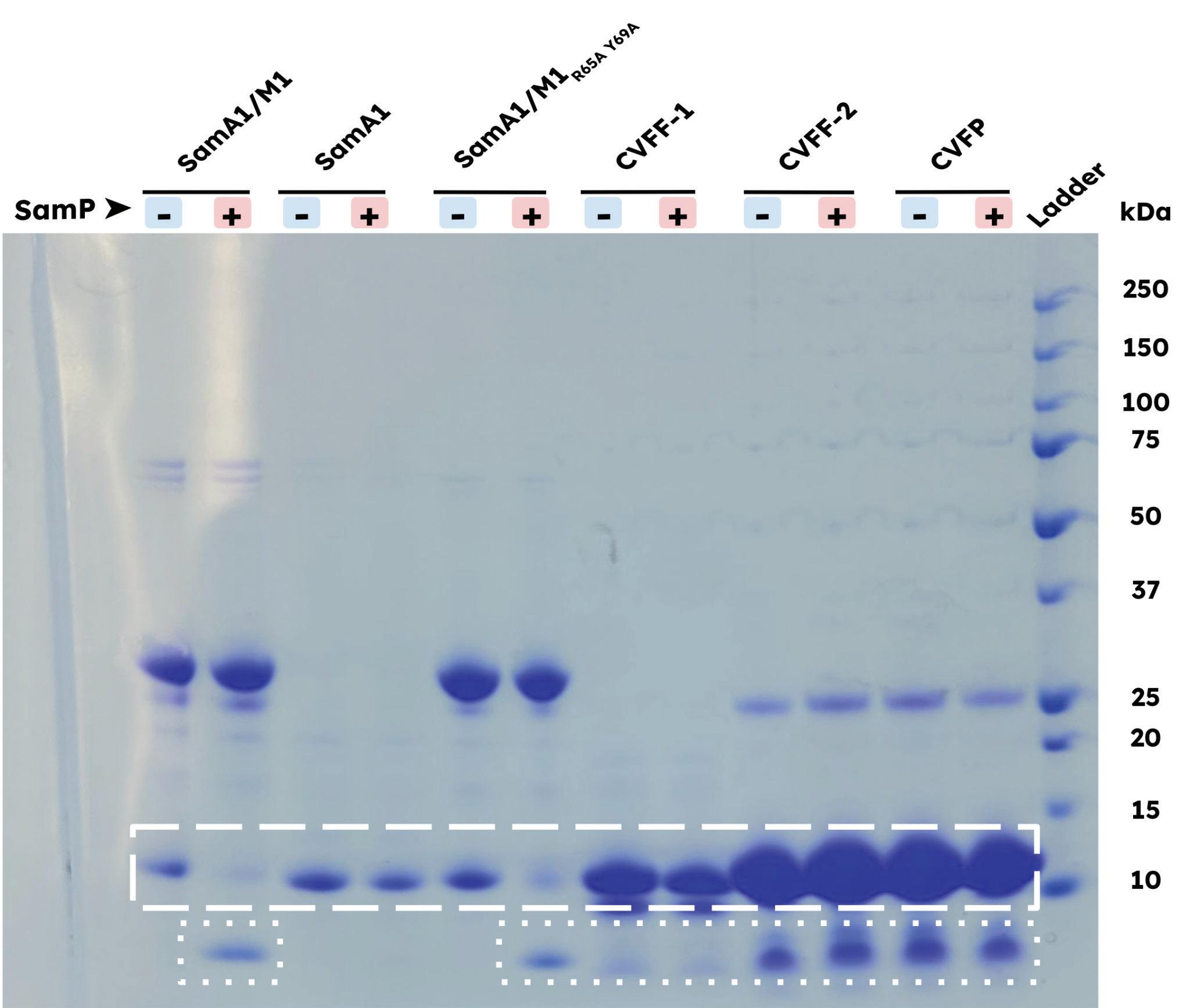
Figure 1. CVFF/CVFP & SamP activity in vitro assay. Columns indicated “+” were cocultured with SamP, whereas lanes indicated “” contain no SamP. From left to right: His-SamA1 and SamMT complex (SamA1/M1), SamA1, SamA1 and inactive SamMTR65A Y69A mutant (SamA1/M1R65A Y69A), post-SEC methylated SamA1 (CVFF-2), post-SEC unmethylated SamA1 (CVFF-1), and post SEC His-SamA1-CVFP (CVFP) His-SamA1 (~9 5 kDa) is outlined in lines while the cleaved product (~2.8 kDa) is outlined in dots.
will expedite the expression of SamA1 required for gene knockout experiments that will be used to identify and define the rest of the putative enzymes within the Shewanella amazonensis borosin BGC. Bioactivity assays will follow, characterizing the secondary metabolic usage of SamA1 in Shewanella amazonensis and providing any possible applications of the SamA1 final natural product as a drug My research into the mechanisms by which the SamA1 borosin is synthesized and post translationally modified is the first step towards understanding its interactions with the other
enzymes located within the borosin BGC. Further characterization of its bioactivity could lead to the identification of a new, membrane-permeable, protease-resistant, orally bioavailable natural product-derived drug.
Acknowledgments
I would like to acknowledge and sincerely thank Dr. Kati Kragtorp, Dr. Michael Freeman, and Ms. Nisha Vishwanathan for their mentorship and support I would also like to thank the University of Minnesota’s Department of Biochemistry, Molecular Biology, and Biophysics for allowing me to conduct research in their lab.
References
Aslam, B , Wang, W , Arshad, M I , Khurshid, M , Muzammil, S , Rasool, M H , Nisar, M A , Alvi, R F , Aslam, M A , Qamar, M U , Salamat, M K F , & Baloch, Z (2018) Antibiotic resistance: A rundown of a global crisis Infection and Drug Resistance, 11, 1645–1658 https://doi org/10 2147/IDR S173867
Chatterjee, J , Gilon, C , Hoffman, A , & Kessler, H (2008) N-Methylation of Peptides: A New Perspective in Medicinal Chemistry Accounts of Chemical Research, 41(10), 1331–1342 https://doi org/10 1021/ar8000603
Crone, K K , Jomori, T , Miller, F S , Gralnick, J A , Elias, M H , & Freeman, M F (2023) RiPP enzyme heterocomplex structure-guided discovery of a bacterial borosin α-N-methylated peptide natural product RSC Chemical Biology, 4(10), 804–816
https://doi org/10 1039/D3CB00093A
Fleming, A (1929) On the Antibacterial Action of Cultures of a Penicillium, with Special Reference to their Use in the Isolation of B influenzæ British Journal of Experimental Pathology, 10(3), 226–236
Freeman, M F , Vagstad, A L , & Piel, J (2016) Polytheonamide biosynthesis showcasing the metabolic potential of sponge-associated uncultivated ‘Entotheonella’ bacteria Current Opinion in Chemical Biology, 31, 8–14
https://doi org/10 1016/j cbpa 2015 11 002
Lee, A R , Carter, R S , Imani, A S , Dommaraju, S R , Hudson, G A , Mitchell, D A , & Freeman, M F (2024) Discovery of Borosin Catalytic Strategies and Function through Bioinformatic Profiling ACS Chemical Biology, 19(5), 1116–1124
https://doi org/10 1021/acschembio 4c00066
Li, X , Wang, N , Liu, Y , Li, W , Bai, X , Liu, P , & He, C -Y (2023) Backbone N-methylation of peptides: Advances in synthesis and applications in pharmaceutical drug development
Bioorganic Chemistry, 141, 106892
https://doi org/10 1016/j bioorg 2023 106892
Matabaro, E , Kaspar, H , Dahlin, P , Bader, D L V , Murar, C E , Staubli, F , Field, C M , Bode, J W , & Künzler, M (2021)
Identification, heterologous production and bioactivity of lentinulin A and dendrothelin A, two natural variants of backbone N-methylated peptide macrocycle omphalotin A. Scientific Reports, 11, 3541 https://doi org/10 1038/s41598-021-83106-2
Maveyraud, L., & Mourey, L. (2020). Protein X-ray Crystallography and Drug Discovery Molecules, 25(5), 1030 https://doi org/10 3390/molecules25051030
Montalbán-López, M , Scott, T A , Ramesh, S , Rahman, I R , Heel, A J van, Viel, J H , Bandarian, V , Dittmann, E , Genilloud, O , Goto, Y , Burgos, M J G , Hill, C , Kim, S , Koehnke, J , Latham, J A , Link, A J , Martínez, B , Nair, S K , Nicolet, Y , Donk, W A van der (2021) New developments in RiPP discovery, enzymology and engineering Natural Product Reports, 38(1), 130–239 https://doi org/10 1039/D0NP00027B
Quijano, M R , Zach, C , Miller, F S , Lee, A R , Imani, A S , Künzler, M , & Freeman, M F (2019) Distinct Autocatalytic αN- Methylating Precursors Expand the Borosin RiPP Family of Peptide Natural Products Journal of the American Chemical Society, 141(24), 9637–9644 https://doi org/10 1021/jacs 9b03690
Tzvetkov, N T , Kirilov, K , Matin, M , & Atanasov, A G (2024) Natural product drug discovery and drug design: Two approaches shaping new pharmaceutical development Nephrology Dialysis Transplantation, 39(3), 375–378 https://doi org/10 1093/ndt/gfad208
Yuchen Shi
Does Caffeine Help You Study?
Investigating the effects of caffeine on adolescents’ long-term memory and sustained attention
Yuchen Shi
Introduction
Caffeine (1,3,7-trimethylxanthine) is the most widely consumed psychoactive stimulant in the world (Ferré, 2013; Reyes & Cornelis, 2018)
Caffeine naturally occurs in tea and beans and can also be an additive in sodas, but it is most commonly sourced from coffee worldwide (Evans et al., 2024). In a 2024 consumer poll by the National Coffee Association, 67 percent of adults in the U S reported consuming coffee in the past day and 75 percent in the past week (Daily, n d ) Many other types of caffeinated beverages have begun to gain popularity in recent years. One example is energy drinks, which include Monster, Celsius, and Red Bull. Energy drinks aim to assist athletes with their physical performance and endurance by providing large amounts of caffeine, sugar, and other additives and stimulants such as guarana, taurine, and L-carnitine (Costantino et al., 2023).
Since the introduction of Red Bull in the U.S. in 1997, the energy drinks market has grown dramatically (Alsunni, 2015) From 2018 to 2023, energy drink sales in the U S alone have grown by 73 percent (US Energy Drinks Market Report 2024 | Mintel Store, n.d.). The most recent data on adolescents’ caffeine consumption was a study in 2014, which suggested that 26 5 percent of adolescents between 13-17 years old consume coffee on a regular basis (Mitchell et al.). Although anecdotal evidence suggests many adolescents are drinking caffeinated beverages, there has been no published data on caffeine use among adolescents in the past 10 years
A 2018 study reported that the most common reasons for consuming caffeine-containing products were taste, habit, increased alertness, improved social mood, and symptom management (Ágoston et al , 2018) Teenagers likely consume caffeine for similar reasons. A recent poll suggests that the top five reasons

adolescents consume caffeinecontaining beverages are: Caffeine is in their favorite beverages, peers drink them, it helps them stay awake, an early school start, and to help them focus/study (Parents Asleep on Teen Caffeine Consumption?, 2024). Many caffeine-containing products, such as energy drinks, are marketed to improve mental acuity and physical performance (Costantino et al , 2023)
Caffeine is a psychoactive drug, meaning that it can cause changes in mood, awareness, thoughts, feelings, or behavior Some studies have found that caffeine also has an impact on attention, reaction speed, memory, and cognitive function in adults (Borota et al., 2014; Nehlig, 2010; Sherman et al , 2016; Wu et al , 2024; R -C Zhang & Madan, 2021; H Zhang et al , 2020; Loke, 1988), but results are conflicting Borota et al. (2014) found that caffeine affected memory consolidation in adults in an inverted U-shape dose-response curve. Nehlig (2010) found that caffeine has no effect on cognitive functions in adults when materials are learned intentionally Sherman et al (2016) demonstrated that caffeine only improved explicit memory in the mornings and had no effects on memory at any other time of the day in college students Loke found that caffeine had minimal effects on memory and learning in young adults (1988) Wu et al (2024) found that caffeine improved reaction time in adult video game players. R.-C. Zhang & Madan (2021) concluded that there is limited evidence to prove that caffeine benefits functions other than reaction speed
The American Academy of Child and Adolescent Psychiatry suggests limiting caffeine intake to 100 milligrams daily for 12 to 18-year-olds (AACAP, n d ), approximately one 10-oz cup of black coffee. However, this
recommendation is likely based on extrapolation, as very little research has been published on the effects of caffeine on children and adolescents One paper researched caffeine’s effects on children between the ages of 9 and 10 and found that caffeine negatively affects all aspects of cognitive functioning (H. Zhang et al., 2020). One more paper found that caffeine acutely and dose-dependently improved sustained attention among adolescents between the ages of 12 and 17 (Cooper et al , 2021) However, the lack of information shows that more research is needed to determine whether caffeine is truly beneficial for cognition or memory in adolescents
Furthermore, one study also indicates that excessive caffeine intake can lead to mild adverse effects such as anxiety, restlessness, fidgeting, insomnia, facial flushing, increased urination, irritability, muscle twitches or tremors, agitation, tachycardia or irregular heart rate, and gastrointestinal irritation (Evans et al., 2024). Due to potential side effects from excess intake, the FDA recommends a limit of 400 milligrams daily, about four to five cups of coffee, for adults’ caffeine intake (Commissioner, 2023)
Caffeine is absorbed quickly after consumption, reaching peak plasma caffeine concentration at about 30 minutes after ingestion in healthy adult men (Blanchard & Sawers, 1983) Caffeine is primarily metabolized in the liver when ingested orally. However, the speed of caffeine metabolism can vary due to individual differences in age, gender, diet, hormones, and genetic background (Nehlig, 2018) The CYP1A2 gene accounts for 95 percent of caffeine metabolism (Mahdavi et al., 2023), while the NAT2 gene accounts for the other 5 percent (PubChem, n d ) Individual variations on these two genes can cause different magnitudes of effects and speeds of caffeine metabolism.
Caffeine blocks adenosine receptors, specifically A1 and A2A subtypes, and antagonizes its functions (Cappelletti et al , 2015; Mouro et al , 2017). Adenosine receptors inhibit the release of neurotransmitters such as serotonin, glutamine,
acetylcholine, noradrenaline, and dopamine (McLellan et al., 2016). Inhibiting adenosine receptors causes an increased release of dopamine, noradrenaline, and glutamate (Cappelletti et al , 2015) These neurotransmitters play critical roles in regulating mood, alertness, and cognitive functions (Neurotransmitters, n.d.). Adenosine induces sleepiness by inhibiting the release of these chemicals (Bjorness & Greene, 2009) By blocking the adenosine receptors, caffeine makes individuals feel more awake and attentive. These effects of caffeine can be observed even in low doses, such as those from a single cup of coffee (Cappelletti et al , 2015)
The goal of my research was to determine the patterns and purposes of caffeine ingestion by adolescents between the ages of 14 and 18 and to understand whether caffeine affects long-term memory and sustained attention in adolescents
A survey was sent out to high school students to collect information about respondents’ average caffeine intake and reasons for consuming caffeine The second half of this research was a double-blinded experiment Participants between the ages of 14 and 18 were assessed on the effects of caffeine on their sustained attention and long-term memory. Participants were tested for two sessions. At the beginning of each session, they were given either a placebo or a caffeine pill Their long-term memory and sustained attention were then assessed with a story recall test to assess long-term memory and the California Computerized Assessment Package (CalCAP Reaction Time, n.d.).
Materials and Methods
Phase I: Caffeine Consumption Questionnaire
A Google form was created to gather information about the caffeine intake of students The survey collected information about the students’ frequency and reasons for caffeine consumption and their average amount of caffeine consumed per day
Phase II: Participant Testing
Two types of pills were used in this study: caffeinated and placebo. The caffeinated pills contained 100 mg of caffeine (Regular Strength 100mg Caffeine Pills, 2020), which is the recommended limit for adolescents by the AACAP (AACAP, n d ) The placebo pills contained cellulose and have been used in multiple clinical studies (Zeebo Honest Placebo, n.d.). The pills were placed in a pillbox by the mentor and were coded A script was created for each session to ensure consistency in communicating instructions to the participants For the same purpose, a recording of the mentor reading each of the two short stories from the story recall test was also made Furthermore, to make this experiment double-blinded, the mentor assigned each participant a random number and assigned rotating combinations of stories and pills for each participant to ensure an equal distribution of each combination. The participants and the student researcher were not informed of the number and combination of the stories and pills
Individual participants came to the Breck School campus during scheduled times before 11:00 am to reduce the chances of insomnia resulting from caffeine ingestion Participants were asked not to consume any caffeine-containing food, beverages, or pills in the 24 hours before participating in the study or during the three days of the study
Session 1. At the beginning of the first session, the participants were given either a placebo pill or a 100 mg caffeinated pill, along with an 8-oz bottle of water Participants were instructed not to look at the pill while putting it in their mouths.
The participant then waited in a quiet room, under observation, for 30 minutes, watching an episode of Modern Family as a distraction task while waiting for the caffeine to take effect. After 30 minutes, they were asked to follow the Passive Drool Method (Best Practices for Saliva Collection | TCU Eos BioAnalytics, n d ) to collect their saliva sample for the caffeine detection test (Phase III). About 2 mL of the
participants’ saliva was collected in a Saliva Collector Kit (Saliva Collection Kit, n.d.). Collected samples were labeled and stored at -20ºC until they were used for the caffeine detection test
The participants were then given the first round of the story recall test The story recall test was modified from an online published article that demonstrated its effectiveness in assessing the participants’ episodic memory (Martinez, 2023). Two short stories from the article were used. I played a 30-second recording of either short story (designated A or B; Martinez, 2023), and the participants were instructed to listen carefully to the recording Then, they were asked to briefly summarize the Modern Family episode as a distraction task. Afterward, the participants were asked to recall what they remembered from the short story, and their response was scored following the guidelines in the article from which the short stories were used (Martinez, 2023). Each story contained details that were either central or peripheral, and depending on the participants’ responses, each detail was given a score of 0, 0 5, or 1 The score for each detail was determined by the accuracy of the wording of the responses of the participants. Every single detail was given a score of 1 if the participant used exact wording from the original story; a score of 0 5 was given if the participant used partially correct wording or similar concepts but different words from the original story; and a score of 0 was given if the participant did not state the detail or stated a different detail from what was in the original story. Scores were summed for central, peripheral, and total details
Next, the participants completed the Standard Test of the California Computerized Assessment Package (CalCAP; CalCAP Reaction Time, n d ) The CalCAP test is a publicly available test that assesses the test taker's reaction speed and sustained attention using ten subtasks. This test took approximately 20-25 minutes. The CalCAP test showed instructions on a computer screen Participants were asked to read the instructions carefully and press the spacebar when certain symbols appeared on the screen
Yuchen Shi
The CalCAP test included ten subtasks–Simple Reaction Time (RT) 1: Dominant hand, Simple RT: Nondominant Hand, Choice Reaction Time - Digits, Sequential RT 1, Language Discrimination, Simple RT 2: Dominant Hand, Degraded Words with Distract, Response Reversal - Words, Form Discrimination, Simple RT 3: Dominant Hand. Their reaction speeds for all 10 subtasks from the CalCAP task and the response accuracy for six of the tasks (Choice Reaction Time - Digits, Sequential Reaction Time 1, Language Discrimination, Degraded Words with Distract, Response ReversalWords, Form Discrimination) were recorded. After the CalCAP test, the participants were asked to recall the previous short story again, and their responses were scored as previously described.
The participants were asked to return 24 hours later and asked to recall the short story again Responses were again scored as previously described.
Session 2 The procedure from Session 1 was repeated, except the pill and story were different In all cases, Session 2 began immediately following the 24-hour recall at the end of Session 1
Saliva Sample ELISA
Saliva samples were analyzed for caffeine content with an ELISA test according to the manufacturer’s directions (Neogen). Absorbance was measured at 450 nm (Byonoy Absorbance 96 plate reader).
Results and Discussion
Phase I: Caffeine Use Survey
A total of 74 students answered the survey Of the 74 respondents, 70 consumed caffeine at least once in the last 30 days. Out of those respondents, 21 consume caffeine every day, 8 consume 5-6 days a week, 13 consume caffeine 3-4 days a week, 14 consume caffeine 1-2 days a week, and 14 consume caffeine less than once a week (data not shown)
Respondents also reported the types of caffeinated beverages or food they consumed (data not shown) The answers were categorized into one of eight categories: coffee, tea, cola, sports drinks (including pre-workout), energy drinks containing sugar, sugar-free energy drinks, chocolate, and Starbucks caffeinated drinks (other than coffee). Coffee was the most common category, reported by about 43% of the participants who consumed caffeine After this, the most common category was sugar-free energy drinks, consumed by about 21% of the caffeine-consuming participants.
The survey also collected responses about the respondents’ reasons for consuming caffeine The most commonly reported reason was that the beverage or food containing caffeine tasted good, with 29 3% of respondents choosing this answer A total of 37% of the respondents also reported that they consume caffeine to help them stay awake or focused (Figure 1). There were two responses that chose “other”; one responded that caffeine helps with their ADHD, and the other responded that caffeine gives them energy to focus, study, and work out
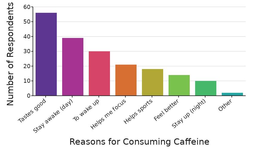
Figure 1. The respondents’ reported reasons for consuming caffeine Figure by author
Phase II: In-person testing Participant Demographics Ten high school students participated in Phase II of the research. Six were male, and four were female. The participants ranged from fourteen to eighteen years old
Story Recall. Participants were tested on long-term memory with the Story Recall Test. An audio of a short story was played to the
Yuchen Shi
participants, and they were asked to remember as many details as possible. A distraction task was conducted to ensure the story was encoded into their long-term memory After the distraction task, they were asked to recall the story three times: immediately after the distraction task, 30 minutes after hearing the story, and 24 hours after hearing the story. Two stories were given in an alternating order to participants, with half of the participants hearing story A during their first session and the other half receiving story B; half received caffeine during the first session, and the other half received the placebo. Recall of the stories immediately after the distraction task, 30 minutes after hearing the story initially, and 24 hours after hearing the story were assessed for both peripheral and central details. Although the stories were meant to be similar, participants who received Story B during the first session did significantly worse at the 24-hour time point on recalling central, peripheral, and total details (a sum of scores for both peripheral and central details) than those who received story A (p<0.01; ANOVA with Tukey post-hoc; Figure 2), though there was no difference between story A and story B during the second session (p = 0 79, ANOVA) This indicated that Story B could be more difficult to recall than Story A, causing the participants who received Story B in Session 1 to have a lower score if they heard it during the first time they completed the task
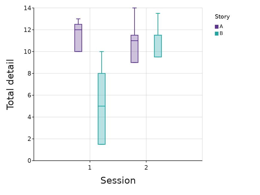
Figure 2. Relationship between session and story type on total detail scores at 24 hours after testing n = 5 for each treatment/story combination. Figure by author.
The participants’ peripheral detail recall scores also significantly decreased in session 2 compared to session 1, both immediately after the distraction task and 24 hours after (data not shown)
The raw scores for central, peripheral, and total (combined) detail were not significantly different between the caffeine and placebo groups immediately after hearing the story, 30 minutes after hearing the story, or 24 hours after hearing the story (Data not shown). However, since each individual had a different level of recall the first time they heard the story, and due to the known impact of having story B first on the raw scores and the average session peripheral recall scores, the scores were then normalized for further analysis by dividing the 30 minute and 24 hour recall scores by the immediate recall scores for that session There was a significant increase in the normalized central detail scores in the caffeine treatment group as compared to placebo treatments 24 hours after the participants initially heard the short stories (Figure 3). One participant scored a zero in their first recall, so their normalized data was excluded from the results
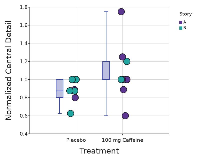
Figure 3. Proportion of change in central detail score (Normalized central detail) at 24 hours as compared to each participant’s immediate central detail score for placebo and caffeine treatments. Purple dots show participants who heard story A, and green dots show participants who heard story B Placebo with story A, n = 4; Placebo with story B, n = 5; 100 mg Caffeine with story A, n = 5; 100 mg Caffeine with story B, n = 4. Figure by author.
CalCAP test for attention
The mean reaction speed of each participant for each test from the CalCAP program was compared between placebo and caffeine treatments. There was no significant difference in the means from each test (data not shown)
Sustained attention was assessed by comparing the change in reaction time throughout the CalCAP test The Simple Reaction Time-Dominant hand test (Simple RT-Dom) was repeated three times throughout the test, and the participants' reaction time for each test was compared between treatments The overall change in reaction time under caffeine was not significant (p=0 35; ANOVA; data not shown)
Phase III: ELISA testing
An ELISA test was performed on the participants’ saliva samples to test their actual caffeine levels The average calculated concentration for the placebo samples was 94 13 ng/mL, and the average calculated concentration for the caffeine samples was 91.18 ng/mL. However, the concentration was much closer than expected; therefore, the level of caffeine was not considered for the comparison of data, and the treatment was determined based on the prerecorded information by the mentor.
Discussion
Phase I
The results from the online survey demonstrate that high school students are consuming caffeine regularly 29 16% of the respondents to the survey consume caffeine every day, and a total of 77.76% of the respondents consume caffeine at least once per week. The survey responses also suggest that, besides liking the taste of the caffeinated beverages, the most common reason for the students to consume caffeine was to stay focused while studying or stay awake during the day. This indicates that many students believe that caffeine has a beneficial effect on their learning. In general, the survey established the popularity of caffeine among high school
students and some of the common conceptions high school students have about caffeine.
Phase II
The central detail scores of participants when recalling the stories 24 hours after exposure were significantly higher in the presence of caffeine as compared to placebo. This was the only place where there was a significant difference between data, indicating that caffeine likely has little to no effect on learning overall Although there was also a significant difference between the peripheral detail scores of participants from immediately after listening to the stories and 24 hours after, this was likely due to the difference in difficulty between Story A and Story B All participants who received Story B in Session 1 had a much lower score than participants who received Story A in Session 1, indicating that Story B is likely to be more difficult to memorize than Story A.
Reaction time was measured using the CalCAP test. The reaction time for each test was not significantly different between the placebo and caffeine groups This is different from the general result from other experiments conducted on adults, where caffeine significantly improved reaction time (Adan & Serra‐ Grabulosa, 2010; Killgore et al., 2009; McLellan et al., 2016; Wu et al., 2024).
The three repeated Simple Reaction Time-Dominant Hand test (Simple RT-Dom) scores were compared to see how the participants’ reaction time changed, to measure sustained attention There was no significant difference in the change in reaction time between the placebo and caffeine groups, indicating that caffeine does not have a significant effect on sustained attention. This result differs from another study on caffeine’s effects on sustained attention in adolescents between the ages of 12 and 17, where caffeine showed an acute and dose-dependent improvement (Cooper et al., 2021). However, Copper et al. conducted experiments with different amounts of caffeine (1mg/kg, 3mg/kg, and 5mg/kg), with the median amount of
caffeine consumed per day being 28 mg, and they did not use the CalCAP test. Since the dosage of caffeine used in this research is much higher and the attention test is different, the data can lead to different conclusions
Phase III
Caffeine metabolizes at different speeds among individuals, causing variations in its effects (Nehlig, 2018) So, an ELISA test was conducted on the saliva samples collected from the participants to measure the specific levels of caffeine in each participant with the intention of accounting for this variation. However, although the procedures were followed thoroughly, constant non-specific binding occurred in the samples, giving consistently high readings for all samples After attempting changes in sample preparation and detection procedures that yielded the same results, the treatment each participant received was used for analysis instead Thus, it is possible that some differences in the actual effects of caffeine were missed due to individual variations in caffeine metabolism Measuring caffeine levels in blood samples would likely be more effective, which would require the assistance of trained medical professionals and is outside the scope of this study
Conclusion
This preliminary research was limited to a small population. Because almost no research on the topic has preceded this research, it cannot be concluded that the results can reflect the trend in the general population Furthermore, this research only reports the correlation between caffeine and long-term memory and sustained attention. Other elements of cognitive functions and learning could be affected in different ways. Future research should use a larger sample of participants and assess caffeine’s effects on other aspects of cognitive functions and learning, such as motor skills and processing speed.
This research is the first to investigate the effects of caffeine on adolescents’ learning and contributes to an initial understanding of how caffeine might affect adolescents’ learning
abilities. Future research is needed to expand on these results, allowing a more profound understanding to help establish proper guidelines for adolescents’ caffeine consumption
Acknowledgments
I want to thank Dr. Kati Kragtorp for helping me through this research project with guidance, advice, and support.
References
AACAP (n d ) Caffeine and Children Retrieved May 29, 2024, from https://www aacap org/AACAP/Families and Youth/Facts for Fa milies/FFF-Guide/Caffeine and Children-131 aspx
Ágoston, C , Urbán, R , Király, O , Griffiths, M D , Rogers, P J , & Demetrovics, Z (2018) Why Do You Drink Caffeine? The Development of the Motives for Caffeine Consumption Questionnaire (MCCQ) and Its Relationship with Gender, Age and the Types of Caffeinated Beverages. International Journal of Mental Health and Addiction, 16(4), 981–999 https://doi org/10 1007/s11469-017-9822-3
Alsunni, A A (2015) Energy Drink Consumption: Beneficial and Adverse Health Effects International Journal of Health Sciences, 9(4), 468–474
Best Practices for Saliva Collection | TCU Eos BioAnalytics (n d ) Retrieved June 6, 2024, from https://bioanalytics tcu edu/best-practices-for-saliva-collection/
Bjorness, T E , & Greene, R W (2009) Adenosine and Sleep Current Neuropharmacology, 7(3), 238–245 https://doi org/10 2174/157015909789152182
Blanchard, J , & Sawers, S J (1983) The absolute bioavailability of caffeine in man European Journal of Clinical Pharmacology, 24(1), 93–98 https://doi org/10 1007/BF00613933
Borota, D , Murray, E , Keceli, G , Chang, A , Watabe, J M , Ly, M , Toscano, J P , & Yassa, M A (2014) Post-study caffeine administration enhances memory consolidation in humans Nature Neuroscience, 17(2), 201–203 https://doi org/10 1038/nn 3623
CalCAP Reaction Time (n d ) Retrieved May 23, 2024, from https://www calcaprt com/calcap htm
Cappelletti, S , Daria, P , Sani, G , & Aromatario, M (2015) Caffeine: Cognitive and Physical Performance Enhancer or Psychoactive Drug? Current Neuropharmacology, 13(1), 71–88 https://doi org/10 2174/1570159X13666141210215655
Cooper, R K , Lawson, S C , Tonkin, S S , Ziegler, A M , Temple, J L , & Hawk, L W (2021) Caffeine enhances sustained attention among adolescents Experimental and Clinical Psychopharmacology, 29(1), 82–89 https://doi org/10 1037/pha0000364
Costantino, A , Maiese, A , Lazzari, J , Casula, C , Turillazzi, E , Frati, P , & Fineschi, V (2023) The Dark Side of Energy Drinks: A
Comprehensive Review of Their Impact on the Human Body Nutrients, 15(18), 3922 https://doi org/10 3390/nu15183922
Daily (n d ) Retrieved July 21, 2024, from https://www ncausa org/Newsroom/Daily-coffee-consumption-at-2 0-year-high-up-nearly-40
Evans, J , Richards, J R , & Battisti, A S (2024) Caffeine In StatPearls StatPearls Publishing http://www ncbi nlm nih gov/books/NBK519490/
Ferré, S (2013) Caffeine and Substance Use Disorders Journal of Caffeine Research, 3(2), 57–58 https://doi org/10 1089/jcr 2013 0015
Loke, W H (1988) Effects of caffeine on mood and memory Physiology & Behavior, 44(3), 367–372 https://doi org/10 1016/0031-9384(88)90039-X
Mahdavi, S , Palatini, P , & El-Sohemy, A (2023) CYP1A2
Genetic Variation, Coffee Intake, and Kidney Dysfunction JAMA Network Open, 6(1), e2247868 https://doi org/10 1001/jamanetworkopen 2022 47868
Martinez, D (n d ) Story Recall Rubric Retrieved June 10, 2024, from https://osf io/u3zev/
Martinez, D (2023) Scoring Story Recall for Individual Differences Research: Central Details, Peripheral Details, and Automated Scoring https://doi org/10 31234/osf io/u64va
McLellan, T M , Caldwell, J A , & Lieberman, H R (2016) A review of caffeine’s effects on cognitive, physical and occupational performance Neuroscience & Biobehavioral Reviews, 71, 294–312 https://doi org/10 1016/j neubiorev 2016 09 001
Mitchell, D C , Knight, C A , Hockenberry, J , Teplansky, R , & Hartman, T J (2014) Beverage caffeine intakes in the U S Food and Chemical Toxicology, 63, 136–142 https://doi org/10 1016/j fct 2013 10 042
Mouro, F M , Batalha, V L , Ferreira, D G , Coelho, J E , Baqi, Y , Müller, C E , Lopes, L V , Ribeiro, J A , & Sebastião, A M (2017) Chronic and acute adenosine A2A receptor blockade prevents long-term episodic memory disruption caused by acute cannabinoid CB1 receptor activation Neuropharmacology, 117, 316–327 https://doi org/10 1016/j neuropharm 2017 02 021
Nehlig, A (2010) Is Caffeine a Cognitive Enhancer? Journal of Alzheimer’s Disease, 20(s1), S85–S94 https://doi org/10 3233/JAD-2010-091315
Nehlig, A (2018) Interindividual Differences in Caffeine Metabolism and Factors Driving Caffeine Consumption Pharmacological Reviews, 70(2), 384–411 https://doi org/10 1124/pr 117 014407
Neurotransmitters: What They Are, Functions & Types (n d ) Cleveland Clinic Retrieved July 15, 2024, from https://my clevelandclinic org/health/articles/22513-neurotransmitt ers
Parents asleep on teen caffeine consumption? (2024, May 20)
National Poll on Children’s Health https://mottpoll org/reports/parents-asleep-teen-caffeine-consumpti on
PubChem (n d ) NAT2 N-acetyltransferase 2 (human) Retrieved July 8, 2024, from https://pubchem ncbi nlm nih gov/gene/NAT2/human
Regular Strength 100mg Caffeine Pills (2020, October 20) Jet-Alert https://jet-alert com/products/jet-alert-regular-strength-caffeine/
Reyes, C M , & Cornelis, M C (2018) Caffeine in the Diet: Country-Level Consumption and Guidelines Nutrients, 10(11), 1772 https://doi org/10 3390/nu10111772
Saliva Collection Kit (n d ) Filtrous Retrieved July 18, 2024, from https://filtrous com/products/saliva-collection-kit-with-funnel-and10ml-tube-sterile-25-unit
Sherman, S M , Buckley, T P , Baena, E , & Ryan, L (2016) Caffeine Enhances Memory Performance in Young Adults during Their Non-optimal Time of Day Frontiers in Psychology, 7 https://doi org/10 3389/fpsyg 2016 01764
US Energy Drinks Market Report 2024 | Mintel Store (n d ) Retrieved August 1, 2024, from https://store mintel com/us/report/us-energy-drinks-market-report/
Wu, S -H , Chen, Y -C , Chen, C -H , Liu, H -S , Liu, Z -X , & Chiu, C -H (2024) Caffeine supplementation improves the cognitive abilities and shooting performance of elite e-sports players: A crossover trial Scientific Reports, 14, 2074 https://doi org/10 1038/s41598-024-52599-y
Zeebo Honest Placebo (n d ) Zeebo® USA Retrieved June 5, 2024, from https://zeeboeffect com/
Zhang, H , Lee, Z X , & Qiu, A (2020) Caffeine intake and cognitive functions in children Psychopharmacology, 237(10), 3109–3116 https://doi org/10 1007/s00213-020-05596-8
Zhang, R -C , & Madan, C R (2021) How does caffeine influence memory? Drug, experimental, and demographic factors Neuroscience & Biobehavioral Reviews, 131, 525–538 https://doi org/10 1016/j neubiorev 2021 09 033
Health Evaluation Robot for Basil – HERB
A modular robotic system for detecting nutrient deficiency in greenhouse basil
Allie Sigmond and Benny Marmor
Introduction
Currently, agriculture is plagued with a multitude of issues surrounding the accessibility of food in cities Today, worldwide population increase outpaces the rise of food production, so much so that food production will need to double to support the estimated 2050 population, 68% of whom are expected to reside in cities (Jonathan Foley, n.d.; University of Michigan, n d ) Food transportation is also unfavorable, as supply chain issues have been shown to significantly decrease the availability of nutritional produce in cities, and the transportation of food accounts for as much as an equivalent 3 gigatons of CO2 emitted annually (Kakaei et al , 2022; Li et al , 2022)
To sustainably meet the demand for food in cities, urban agriculture, the practice of growing food crops in urban environments, including in greenhouses, has become an increasingly promising solution Urban agriculture has the potential to mitigate supply chain issues, increase food security, decrease carbon emissions, and cool cities (Urban Agriculture | USDA Climate Hubs, n d ) However, its high cost makes it difficult to implement at a large scale Greenhouses are also a promising solution to increasing food production due to the ability to bring fresh produce to urban centers without a large environmental cost from transportation (Field to Fork, n d ; Urban Agriculture | USDA Climate Hubs, n d ) To increase crop production and meet the increasing demand for food, crop production needs to be made more efficient; making more efficient and productive greenhouses will greatly aid in this endeavor.
Crop production is generally time and labor-intensive, as farmers must spend up to 70% of their time monitoring plant health (Khan et al , 2020) Human crop monitoring overall is

inefficient due to high cost and low speed, stemming from the fact that specially trained people must individually check each plant for problems To address this issue, research on autonomous crop monitoring has grown exponentially in recent years. Development of each monitoring system must address three, related issues: 1) the physical means of navigating the planted area to collect information, 2) the method of detection and, 3) the method of analysis that can lead to identification of deficiency.
Concerning the method of surveying the crops, most systems focus on satellite or unmanned aerial vehicle (UAV) applications for use on outdoor crops (Barbedo, 2019; Ma et al., 2022). The greenhouse environment, with its limited space and visibility through greenhouse roofs, makes UAVs and satellites unusable for greenhouse spaces and poses unique challenges unseen in other plant growth mediums. Thus, for many applications, an unmanned ground vehicle (UGV) is the best option, allowing detailed imagery and a more versatile operation However, most of these machines were all designed for field operation, meaning they are generally wide, bulky, and low to the ground, rendering them unable to scan greenhouse plants in tight spaces and tables (Sowing Seeds of Change, n d ) Carts on ceiling-mounted rails can capture images in greenhouses, however, this type of system is costly and requires specialized tracks for implementation.
UGVs for greenhouse applications have generally been designed to apply pesticides or fertilizer to plants rather than to capture images (Asefpour Vakilian & Massah, 2012; Feng et al., 2020; Hu et al , 2022; Ruckelshausen et al , 2009) In 2021, Hasuda and Keita designed an autonomous robot that can traverse greenhouse aisles. Their machine was designed to precisely
Allie Sigmond and Benny Marmor
spray pesticides on greenhouse plants to reduce the amount of pesticide used overall (Yuichi Hasuda & Hirayama Keita, 2021, 2021)
Far less research has been done in the area of UGVs for nutrient deficiency detection. Asefpour Vakilian & Massah (2012) created a robot able to detect nutrient deficiencies in greenhouse cucumbers two days earlier than humans (Asefpour Vakilian & Massah, 2012) Nadazadeh et al. (2024) created a robot that could detect iron deficiency in greenhouse spinach with 83% accuracy, 3% higher than experts checking the plants (Nadafzadeh et al , 2024) Current research has shown significant promise in the development of greenhouse robotics. The major drawback to each greenhouse robot currently is that each is designed specifically to operate in a single type of greenhouse, suffering from the same drawback of inflexible design that rail-mounted detection systems have. Additionally, most are completely made out of metal, which is both heavy and expensive. We were unable to find a system that extends above or over plants, meaning canopy size detection (which can reflect a plant’s lack of growth due to nutrient deficiency) cannot be used with these robots. They also cannot look at plants past a row immediately closest to the aisle where a robot is positioned Overall, current designs demonstrate the practicality and accuracy of greenhouse robots in detecting nutrient deficiencies but lack the flexibility and affordability required to be implemented as one standard industry design.
Concerning the methods of analysis used, one option is a multi-sensor approach, combining images on the Red-Green-Blue (RGB) spectrum with those from the near-infrared (NIR) spectrum This allows one to use the Normalised Difference Vegetation Index (NDVI), a commonly used metric for measuring plant health that relies on the red and near-infrared (NIR) bandwidths of light (Stamford et al., 2023). However, this approach is very expensive, causing most UGVs to rely only on various combinations of RGB cameras
When processing proximal images taken by RGB cameras, many systems use various methods of machine learning (ML) A support vector machine (SVM) is primarily used for classification and works by finding a hyperplane that best separates different data points. SVMs are computationally inefficient and are best when there exists a large amount of input data. A regression is used to define the relationship between various independent and dependent variables They are computationally efficient and are supervised, which means that the researcher can know what the inputs are (Zhang, 2010). Others, like computational neural networks (CNNs), are unsupervised Largely used for classification, the inputs a CNN uses to get to its result are unknown CNNs work best for images and work by analyzing small sections of the image to classify objects in the image. Each section is analyzed by passing it through a series of filters that are tuned throughout the training process (Kattenborn et al , 2021) Techniques may be chosen by virtue of convenience with the resources and coding language the researcher is using, and various factors can make ML methods easier to implement or more computationally efficient The researcher may also choose to forgo machine learning altogether and rely on a simple measurement of a plant’s phenotype that is indicative of what the researcher is trying to detect.
Various approaches have been utilized to analyze the health of a plant using proximal imaging. Still, since 2010, only 37 studies have been published using the RGB spectrum. Of these, only three were performed by robots (as opposed to leaves being physically removed from the plant or being imaged by hand) and designed and tested in a greenhouse environment (Asefpour Vakilian & Massah, 2012; Barbedo, 2019; Nadafzadeh et al , 2024) One approach taken by researchers examining methods of detecting nutrient deficiencies in plants specifically, was analysis of the textural features of images. Textural features are a way for a computer to detect different patterns in an image based on the relationships between different pixel intensities (Haralick et al , 1973) The
textural features analyzed were entropy, homogeneity, and contrast (Ushada et al., 2007). Other researchers used Top Projected Canopy Area (TPCA) in conjunction with textural features, which is a measure of the area of the plant from an image taken from the top of the plant. However, the researchers who used this method to detect nutrient deficiency used a mounted cart system that went above the plants, a method that is too expensive to be practical for scale
We designed and built a system specifically tailored to the application of machine learning on nutrient deficiency detection in greenhouses We used a ground-based, autonomous robot capable of navigating between rows of greenhouse tables via the detection of tape lines on the ground The robot successfully navigated by following testing on lines on the ground and the imaging system successfully moved, detected, captured, and sent images of QR codes from a Raspberry Pi to a computer for analysis. Initial trials of images taken manually of hydroponically grown basil produced promising results for the use of Top Projected Canopy Area (TPCA) as a measure of nutrient deficiency This flexible design is capable of collecting imaging data for other methods and analysis, like textural features, and was designed to operate seamlessly in most greenhouse environments The analysis methods described here serve as a proof of concept for this approach, and could eventually be expanded to a variety of crops.
Materials and Methods
Robot CAD
A complete version of the robot was designed in Solidworks 2023, a CAD software created by Dassault Systèmes The robot was designed to rise above and extend over the rows of plants, where a cart with a camera could then be used to take birds-eye photos of basil plants for analysis (Figure 1).
Allie Sigmond and Benny Marmor
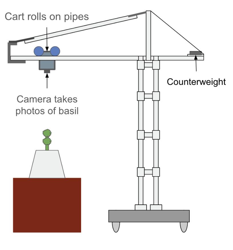
Arm
A vertical arm connects the chassis to the boom Rigidity was crucial to the stability of the boom, to maximize the quality of pictures and data We used 1.5" ID Schedule 40 PVC pipe as our primary building material due to its low cost, wide availability, toughness, and ease of building The arm consists of four of these pipes held together by groups of eight PVC T-fittings (square joints) The pipes were placed in a square configuration for maximum stability and ease of mounting. Each square joint consists of eight fittings, two on each corner, held flush and concentric with each other at a 90-degree angle with PVC cement and a pipe attached between them. Corners are attached to each other with 1.5" OD PVC pipe so that the 4 corners create an 8.25x9.25-in center-to-center rectangle. Three of these square joints were installed at intervals of 16" starting from the top so that the final arm height is 76 5" On the top of the arm, a PVC coupling and 1.5" to 0.5" PVC bushing are attached in each hole. Inside the PVC bushing, a 0.5" ID Schedule 40 PVC pipe is attached, just long enough for the boom to be attached flush with the PVC bushings PVC flanges were attached to the bottom of the arm for easy mounting onto the chassis.
Figure 1. Schematic of the robot Figure by authors
Boom
The boom is the horizontal assembly that reaches over the greenhouse tables. Mounted to the boom is a sensor cart, which houses the camera Since photos needed to be taken at a consistent height, a rigid material, 1 5" ID Schedule 40 PVC, was the primary building material for the boom. The boom consists of the center mounting area, the front pipes, and the back pipes. The center mounting area includes 4 down-facing PVC T-fittings used to attach the boom to the arm These T-fittings are held at 8 25 and 9 25" distances center-to-center by additional PVC pipe T-fittings, mounted perpendicular, flush, and concentric to the down-facing fittings with PVC cement, similar to the corners of the arm’s square joints The center mounting area also includes two upright pipes, kept together by two 90-degree PVC fittings and a PVC pipe.
Since the robot needed to extend very far in one direction to look over the plants, the front pipes were much longer than the back pipes. The front pipes consist of two 1.5" ID Schedule 40 PVC pipes attached to the T-fittings of the center mounting area The ends of the pipes are held together by two 90-degree fittings and another PVC pipe Attached to the end of the pipes is a U-shaped 0.25" thick aluminum bracket. Between the end of this bracket and the top of the upright pipes, a 0 5" diameter PVC pipe was attached with 9" long aluminum pieces at each end
Back pipes and a counterweight were added to act as a counterweight to the front pipes to balance the weight of the front pipes They are much shorter than the front pipes and are joined together by two pipes at the very end. A rope was tied between the end of the back pipes and the upright pipes.
Sensor Cart
The sensor cart houses the RPi and camera, which are responsible for taking photos of the basil plants (Figure 3) Mechanically, it consists of three sets of wheels attached to two 375" thick polycarbonate plates. Two sets of wheels
run horizontally and are attached to the polycarbonate plates with 32mm length U brackets (Tetrix). Under each U bracket are 3 0 75" metal spacers in an arrow configuration One set of these horizontal wheels is attached to a 26cm long 6mm D-shaft axle, centered on the polycarbonate plates, on which a 3" diameter nub bore 50A durometer wheel (Andymark) is attached at each end. This axle runs through two of the U brackets and is at the front of the sensor cart Centered on the top of the sensor cart, mounted by a Tetrix motor mount (Tetrix) on top of 2 0 5" spacers, is a Torquenado motor 6mm D-shaft bevel gears (Tetrix) are attached to both the Torquenado motor and the 6mm D-shaft axle at the front of the sensor cart These gears are meshed so that when the motor rotates, the wheeled axle does as well, pulling the cart forward or backward. In the back of the sensor cart, a second set of horizontal wheels guarantees the horizontal stability of the sensor cart Each wheel is attached to its own axle since the Torquenado motor extends too far back for one axle to be run through Both axles were secured each by one U bracket and had a 3" diameter nub bore 50A durometer wheel (Andymark) attached. Each horizontal wheel was aligned so that each was the same distance from the center of the polycarbonate plates An appropriate bushing and motor hub (Tetrix) was attached at any point where a horizontal axle was held by a U bracket.
The other set of wheels runs vertically between the polycarbonate plates They consist of four, 2" diameter, 0 5" hex bore 50A durometer wheels (Andymark), each on a corner of the sensor cart. Each vertical axle is a 2" long 0.5" hex axle, and is attached to the polycarbonate plates with 0 5" hex bearings (McMaster-Carr) A wheel is placed in the middle of each axle The spacers and wheel are then placed between the polycarbonate plates Each polycarbonate plate was cut using a CNC machine.
The RPi is mounted on a section of the bottom plate that extends out of the back An RPi camera is placed in a hole in the center of the bottom plate A thin polycarbonate shield with a hole for wires extends from the bottom plate and covers the entire top of the sensor cart.
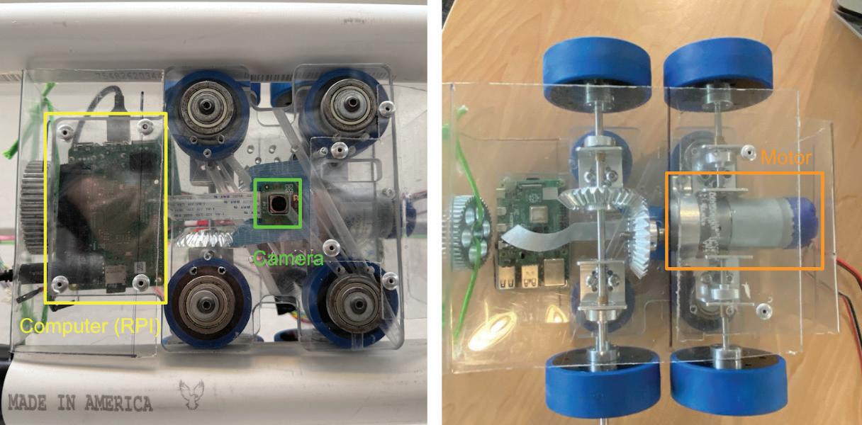
2. Bottom (a) and top (b) view of the sensor cart Figure by authors Inside the yellow square is the RPi The green square contains the camera, and the orange square contains the motor.
Chassis
Due to the heavy weight of the arm and boom, the chassis needed to be extremely stable, rigid, and able to operate on the uneven ground of a greenhouse With this in mind, we chose 2x1" aluminum tube stock with 0 125" thick walls as our primary building material The chassis frame was assembled as a 22x31 5" rectangle with two pieces of aluminum stock inside creating two 3-inch gaps inside of the chassis. The aluminum stock was assembled with gussets and rivets Axles were run between the 3-inch gaps, on which we put the wheels (Figure 3) We chose CIM motors (Andymark) mounted 2" offset from the center of the robot for our drive motors due to their low cost and high performance. A 25:1 MAX planetary gearbox (REV Robotics) is mounted to each motor The output shaft for the motors and the wheel axles are all 0 5" aluminum hex shafts. We chose Smoothgrip wheels (Andymark) for our drive wheels for their large size and compatibility with 0.5" hex shaft The motor and wheel axle were connected with pulleys with a 6/15 gear ratio Each drive axle and motor shaft is tapped and secured with bolts. Each drive axle has its wheel placed on the far end of the axle and its pulley on the close end of the axle, with a 0.5" HEX spacer (VEX Robotics) separating them On top of the center of the chassis is a polycarbonate sheet, with spacers so the sheet does not touch the motors
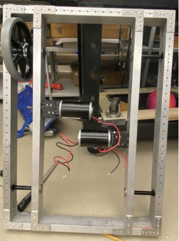
Allie Sigmond and Benny Marmor
Figure 3. Chassis Frame The interior stock is 28" long, parallel to the long side of the chassis frame. Figure by authors
RPi
To control our robot and send images to the laptop, we used an RPi, a computer with a small form factor that includes GPIO (General Purpose Input/Output) pins which allow the RPi to control devices through digital and analog input/output signals. The RPi also includes USB ports, allowing serial communication between the RPi and an Arduino Uno microcontroller board, as well as a ribbon cable port for a camera. As the RPi 3B+ has only two pins with PWM (Pulse Width Modulation) capabilities, we used an Arduino Uno as a helper board; it features six pins with PWM capabilities To interface with the RPi we used both a monitor, keyboard, and mouse, and a combination of SSH (Secure Shell Protocol) and VNC (Virtual Network Computing). Currently, the RPi draws power from a laptop kept on the robot for convenience, but it could draw power from the motor control system
Motor Control System
To control the motors of our robot we used an Arduino Uno microcontroller board, which consists of a series of GPIO pins as well as a USB jack for serial communication and a barrel jack for power The Uno was used to provide a PWM input to the SPARK MAX motor controllers. The SPARK MAX motor controllers were used to power the motors in combination with a Zeee 9000 milliamp lithium-ion battery which was chosen for its ease of use and fast charging The Arduino was coded with the Arduino IDE and the code was then uploaded to
Figure
the Uno after which the Uno took commands from the RPi.
Image Processing
We created a program to process an image so it could be analyzed to determine if the basil in the image was nutrient deficient As we sent all images from the RPi to Google Drive via RClone, we used Google Colaboratory (Colab) with its native Google Drive compatibility as the platform for image processing and analysis
Data Collection and Analysis
We collected data from basil plants that we grew in our own hydroponic system. We germinated each plant in a small pot that contained equal parts peat moss and vermiculite The small pot was kept in a bin filled with only water, and then, after it germinated, was moved in the pot to a larger bin, which included a standard hydroponic nutrient solution (FloraGro 2-1-6, General Hydroponics) and water. We took pictures at one-day intervals using a Canon Vixia HF R500 camera
Results and Discussion
Robot Construction, Cost, Ease, and Modularity
A primary goal for the design of the robot was to make it cheap and modular. Replacing the entire boom took two people about 3 minutes. Adjusting the lengths of the boom pipes also took about 2 minutes The main construction materials of the robot are all cheap and widely available Construction of the majority of the robot only required access to basic tools, making the physical building process quick. Overall, the modularity and easy adjustability of the robot proved to be a major advantage of the design
Since one goal for the robot was for it to be easily built, another potential improvement is to make the robot constructible by anybody with access to basic tools Future iterations of this design should be simplified so that this method of using a scale drawing would be viable for builders.
A goal of the boom was to have it be at an even height for consistency when imaging plants
However, since the boom needed to be long, it experienced a lot of bend, in some places as far as 2 inches below where the boom is attached to the arm Using a support beam at the end of the boom helps this issue, but the lack of support in the center leads to some sagging near the middle of the boom pipes. Ideally, a second support would be added to this region. Another way to increase the stability of the pipes would be to use a thicker schedule 80 PVC pipe instead of schedule 40 PVC pipe, so it would likely bend less than the existing boom.
Drive Train Movement
The robot successfully drove on a 3-inch thick line made of black electrical tape on white paper Two line sensors were used to allow the robot to steer back onto the line if it veered off-path The black electrical tape needed to be three inches thick due to the distance between the two line sensors; in future iterations this thickness could be reduced by reducing the distance between the line sensors The drive train worked without problems, and there were no problems with mechanical movement.
QR Codes
After the robot’s movement, the robot’s arm and plant identification system were tested A QR code on a stand was placed next to each basil plant so each plant could be identified The arm moved along the pipes and took pictures every 1.2 seconds. In the course of traversing the arm, the camera would center on detected QR codes. The camera successfully imaged the QR codes with a variance of 7 5% of the total image dimensions in each direction After imaging, the robot’s arm appropriately moved back to the base location. There were no false positives or negatives QR code detection testing. The next step would be to test QR code and line-following together, in a real-world greenhouse environment
Image Processing
We converted the image from RGB to HSV. Although more successful than other methods, there was still noise in the image Once we had a
Allie Sigmond and Benny Marmor
segmented image, we then used the segmented image to calculate the Top Projected Canopy Area (TPCA) Since basil height is variable we chose to measure TPCA not as a number of pixels, but as a percent change between the pixels over time to compensate for this variability.
TPCA Data
We collected a series of daily images of four basil plants: two grown in nutrient-free water and two grown in water with sufficient nutrients With these images, we analyzed the cumulative percent change in TPCA from the first day of image capture, rather than raw TPCA values due to variance in plant heights On day five, the group with nutrients had a growth spurt and grew at about fifty percent higher rate than the group without nutrients. This growth spurt had a compounding effect on the rest of the days (Figure 4). However, the standard deviations of the two treatments were only clearly separated on day nine Importantly, the variance in percent change of TPCA was significantly affected by treatment and day of collection (ANCOVA; p < 0.01). This means that cumulative TPCA is a promising metric that could be used to accurately detect nutrient deficiency in conjunction with our robotic platform However, sin ce we only tested two plants in each category, more data will need to be collected to confirm these observations.
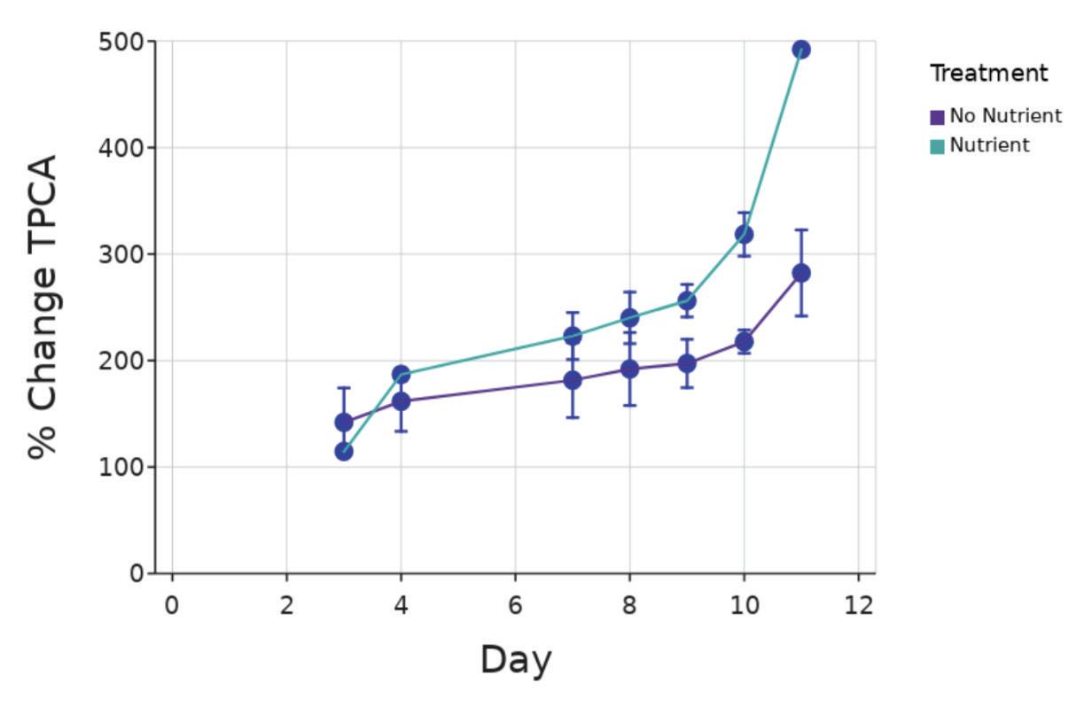
The next steps will be to create a dual-segmented regression model that would be capable of detecting when a plant is nutrient deficient based on its growth trajectory which would allow us to find the inflection point at which growth changes between treatments. Finally, the collection of additional data could give us greater confidence in the promise of percent change TPCA as a variable that could differentiate between deficient and normal growth trajectories; allow us to test our dual-segmented regression model; and allow us to explore the role of other variables, like textural features. Once this model is complete, the final step will be to test it on data collected using the robot This would allow us to ascertain the robot’s capabilities as well as see if the different cameras had an effect on TPCA or on the GLCM features analyzed from the data we currently have.
Conclusions
We collected data indicating that TPCA is a very promising avenue for detecting nutrient deficiency. Additionally, the data we have is amenable to textural analysis, and once we can refine our image masking technique, we hope to also test features extracted from grey-level co-occurrence matrices as a means of detecting nutrient deficiency, utilizing the methods of (Story et al., 2010).
Our robot serves as a proof of concept for a platform that can collect bird's eye view images in a variety of greenhouse environments, regardless of plant type or greenhouse layout. Due to the versatility of our robotic platform, we hope that it can be used for other agricultural applications in addition to nutrient deficiency detection, such as pests or diseases Additionally, we hope that the research we have done on TPCA can serve as a building block for creating models for basil and other plants based on TPCA that allow farmers to diagnose and treat nutrient deficiencies faster, increase their crop yields, and be more efficient in how they farm. Eventually, it may serve as a piece of an agricultural revolution that can sustain a world
Figure 4. Graph of Cumulative Percent Change in TPCA Figure by authors
that will only grow hungrier in its need for sustainable agricultural solutions.
Acknowledgments
We would like to thank Dr Kragtorp, whose advice was invaluable; Dr Yang, from the University of Minnesota’s Department of Bioproducts and Biosystems Engineering for initial project parameters and advice along the way; Jordan Bergstrom, for access to the greenhouse; and Caleb Li, for instrumental coding assistance
References
Asefpour Vakilian, K , & Massah, J (2012) Design, development and performance evaluation of a robot to early detection of nitrogen deficiency in greenhouse cucumber (Cucumis Sativus) With machine vision 2, 448–454
Barbedo, J G A (2019) Detection of nutrition deficiencies in plants using proximal images and machine learning: A review Computers and Electronics in Agriculture, 162, 482–492 https://doi org/10 1016/j compag 2019 04 035
Feng, D , Xu, W , He, Z , Zhao, W , & Yang, M (2020) Advances in plant nutrition diagnosis based on remote sensing and computer application Neural Computing and Applications, 32(22), 16833–16842 https://doi org/10 1007/s00521-018-3932-0
Field to fork: Global food miles generate nearly 20% of all CO2 emissions from food (n d ) Retrieved June 21, 2024, from https://environment ec europa eu/news/field-fork-global-food-miles -generate-nearly-20-all-co2-emissions-food-2023-01-25 en
Haralick, R M , Shanmugam, K , & Dinstein, I (1973) Textural Features for Image Classification IEEE Transactions on Systems, Man, and Cybernetics, SMC-3(6), 610–621 https://doi org/10 1109/TSMC 1973 4309314
Hu, N , Su, D , Wang, S , Nyamsuren, P , Qiao, Y , Jiang, Y , & Cai, Y (2022) LettuceTrack: Detection and tracking of lettuce for robotic precision spray in agriculture Frontiers in Plant Science, 13, 1003243 https://doi org/10 3389/fpls 2022 1003243
Kakaei, H , Nourmoradi, H , Bakhtiyari, S , Jalilian, M , & Mirzaei, A (2022) Effect of COVID-19 on food security, hunger, and food crisis COVID-19 and the Sustainable Development Goals, 3–29 https://doi org/10 1016/B978-0-323-91307-2 00005-5
Kattenborn, T , Leitloff, J , Schiefer, F , & Hinz, S (2021) Review on Convolutional Neural Networks (CNN) in vegetation remote sensing. ISPRS Journal of Photogrammetry and Remote Sensing, 173, 24–49 https://doi org/10 1016/j isprsjprs 2020 12 010
Khan, A., Nawaz, U., Ulhaq, A., & Robinson, R. W. (2020). Real-time Plant Health Assessment Via Implementing Cloud-based Scalable Transfer Learning On AWS DeepLens. https://doi org/10 48550/ARXIV 2009 04110
Li, M , Jia, N , Lenzen, M , Malik, A , Wei, L , Jin, Y , & Raubenheimer, D (2022) Global food-miles account for nearly
20% of total food-systems emissions Nature Food, 3(6), 445–453 https://doi org/10 1038/s43016-022-00531-w
Lin, K , Si, H , Chen, J , & Wu, J (2016) A New Approach for Measuring Leaf Projected Area for Potted Plant Based on Computer Vision In T Tan, G Wang, S Wang, Y Liu, X Yuan, R He, & S Li (Eds ), Advances in Image and Graphics Technologies (Vol 634, pp 1–7) Springer Singapore https://doi org/10 1007/978-981-10-2260-9 1
Ma, Z , Rayhana, R , Feng, K , Liu, Z , Xiao, G , Ruan, Y , & Sangha, J S (2022) A Review on Sensing Technologies for High-Throughput Plant Phenotyping IEEE Open Journal of Instrumentation and Measurement, 1, 1–21 https://doi org/10 1109/OJIM 2022 3178468
Nadafzadeh, M , Banakar, A , Abdanan Mehdizadeh, S , Zare Bavani, M , Minaei, S , & Hoogenboom, G (2024) Design, fabrication and evaluation of a robot for plant nutrient monitoring in greenhouse (case study: Iron nutrient in spinach) Computers and Electronics in Agriculture, 217, 108579 https://doi org/10 1016/j compag 2023 108579
Ruckelshausen, A , Biber, P , Dorna, M , Gremmes, H , Klose, R , Linz, A , Rahe, R , Resch, R , Thiel, M , Trautz, D , & Weiss, U (2009) BoniRob: An autonomous field robot platform for individual plant phenotyping In E J Van Henten, D Goense, & C Lokhorst (Eds ), Precision agriculture ’09 (pp 841–847) Brill | Wageningen Academic https://doi org/10 3920/9789086866649 101
Sowing seeds of change (n d ) The University of Sydney Retrieved July 22, 2024, from https://www sydney edu au/news-opinion/news/2023/12/06/sowing -seeds-of-change html
Stamford, J D , Vialet-Chabrand, S , Cameron, I , & Lawson, T (2023) Development of an accurate low cost NDVI imaging system for assessing plant health Plant Methods, 19(1), 9 https://doi org/10 1186/s13007-023-00981-8
Story, D , Kacira, M , Kubota, C , Akoglu, A , & An, L (2010) Lettuce calcium deficiency detection with machine vision computed plant features in controlled environments Computers and Electronics in Agriculture, 74(2), 238–243 https://doi org/10 1016/j compag 2010 08 010
Urban Agriculture | USDA Climate Hubs (n d ) Retrieved June 21, 2024, from https://www climatehubs usda gov/hubs/international/topic/urban-a griculture
Ushada, M , Murase, H , & Fukuda, H (2007) Non-destructive sensing and its inverse model for canopy parameters using texture analysis and artificial neural network Comput Electron Agric , 57(2), 149–165 https://doi org/10 1016/j compag 2007 03 005
Yuichi Hasuda & Hirayama Keita (2021) Development and Usability Test of Pesticide Spraying Robot for Greenhouse IJERT, 6.
Zhang, Y (Ed ) (2010) New Advances in Machine Learning InTech. https://doi.org/10.5772/225
Unique Creeks
Monitoring Nutrient and Bacteria Levels in Rivers to Determine Factors
Affecting Water Quality
Charlo Vasicek
Introduction
When a body of water does not meet water quality standards, it is considered impaired (Minnesota’s Impaired Waters List | Minnesota Pollution Control Agency, n d ) Impaired waters are polluted enough that they are unsafe for use, such as for drinking water, swimming, or fishing. Several factors can contribute to water impairment, one of which is contamination by fecal coliform bacteria such as Escherichia coli High levels of these bacteria can cause disease in humans and indicate that the water is experiencing excessive contamination (Rytkönen et al., 2024). Efforts to reduce bacterial contamination need to be directed towards reducing a specific cause of contamination, and determining the cause can be difficult Contamination can be caused by human use of the land surrounding a body of water, including livestock farming, crop farming, and wastewater treatment, but wildlife can also be sources of fecal bacteria (Vadde et al , 2019) Another factor contributing to lowered water quality and impairment includes nutrient pollution
There are many factors that can reduce water quality and impact bacteria levels Nutrient pollution, such as by phosphorus or nitrogen, as well as levels of organic material in water, can cause eutrophication and hypoxia, threatening the ecosystem and wildlife (Yang et al., 2008). However, nutrient pollution can also give insight into potential sources of contamination High levels of phosphorus pollution can stimulate not only prolonged survival but also growth of fecal bacteria in rivers (Mallin & Cahoon, 2020). While both phosphorus and nitrogen can be introduced to rivers by fertilizer runoff, another important source of both nutrients is manure runoff from farms, which also introduces fecal bacteria to bodies of water (Alegbeleye & Sant’Ana, 2020). Monitoring nutrient pollution
can help to give a full picture on bacterial impairment Also, since fecal bacteria and nutrient pollution can be introduced to waters from the same source, as with manure runoff, source tracking and reducing sources of bacterial contamination can also reduce levels of nutrient pollution in waters.
Many waters in Minnesota are currently considered impaired by the Minnesota Pollution Control Agency (MPCA). The goal of the MPCA is to prevent and reduce pollution, including water pollution As a result, the MPCA is engaged in several projects to monitor water pollutants, but efforts to track E. coli contamination are falling behind other projects (Bacteria | Minnesota Pollution Control Agency, n d ) The MPCA currently tests for FIB as indicators of pathogens and human health risks in water While these bacteria are easy to test for, the MPCA acknowledges that they are not the best way to determine the presence of pathogens. However, due to the lack of other simple and effective methods to track pathogens, the MPCA states that FIB tracking is its best available option This leaves the MPCA with a lack of information to use in its efforts to reduce fecal bacterial contamination. A first step to understanding Minnesota watershed contamination is to increase coliform and E coli monitoring projects Additionally, since MST markers can present differently in different locations, it is necessary to start testing Minnesota waters to determine which assays are effective
As a part of this effort, Elk River and Mayhew Creek are being monitored for coliform and E. coli counts, as well as being tested for other pollutants Both Elk River and Mayhew Creek are currently considered impaired by the MPCA (Bacteria | Minnesota Pollution Control Agency, n.d.). Samples are taken from sites along the
Charlo Vasicek
rivers and analyzed to collect data about their water quality, levels of certain nutrients, E. coli and total coliform counts The data collected was analyzed to determine trends in bacterial contamination as well as nutrient pollution This should help to determine sources of pollution to these rivers as well as help to predict when water quality tends to be improved, providing information that the MPCA can use in the future to reduce contamination and remove them from the impaired waters list
Materials and Methods
Sample collection
River water samples were collected twice each month in June, July, and August from the watersheds of Minnesota rivers Elm Creek and Elk River Samples were taken from 12 predetermined sites, representative of the watershed Each site was numbered with a three-digit ID to differentiate the sites. Before field work, 24 1 L Nalgene bottles were cleaned in a dishwasher 12 of the cleaned bottles were wrapped individually in foil and autoclaved Autoclaved bottles were used to store samples for DNA and bacterial analysis, and other bottles were used to store samples for chemical analysis. At each site, water was collected from a bridge A bucket was sprayed with 70% ethanol and wiped with paper towels The bucket was tied with rope and thrown into the middle of the river to collect surface water. The bucket was retrieved and the water was swirled around the bucket to rinse it. The bucket was poured out and then thrown again to fill with at least 2 L of water A small amount of water was poured into two 1 L Nalgene bottles, one autoclaved and one not. Lids to the bottles were replaced and the bottles were shaken to rinse all inside surfaces of the bottle. The bottles were then filled with water If a bridge was not available, or if the water level was too low to reach using the rope, the water was collected from the riverbank by throwing the bucket. Bottles containing water samples were kept in a large cooler with ice packs The collection procedure was repeated for each of the 12 sites in the watershed before returning to the lab and storing the coolers at
4℃ . Samples were processed (filtered) within 24 hours of collection. Chemical analysis was either completed within 24 hours of collection, or samples were stored at -20℃ until they could be analyzed
Field testing
Some water tests were completed at the site. When possible, a probe (Thermo Scientific) was used to measure water pH, dissolved oxygen (DO), and temperature When a probe was not available for pH, the pH was measured along with the electrical conductivity (EC) in the lab within 24 hours of sample collection. 100 mL of sample was poured into a sterile 100 mL Colilert bottle (IDEXX) to be used for total coliform and E coli quantification These bottles were stored in a small cooler with ice packs Finally, information about the site was recorded, including the time of sample collection, current air temperature, current precipitation, level of debris in water, stream appearance (color), evidence of E coli source, and type of evidence
Coliform and E. coli count
Immediately after returning to the lab, the 100 mL samples were used for coliform and E coli counting Growth medium powder for use with 100 mL Colilert samples (IDEXX) was added to each bottle and inverted several times to combine. A Colilert Quanti-Tray (IDEXX) was labeled with a sample’s ID number, and that sample was poured into the tray The tray was sealed using a Quanti-Tray Sealer PLUS (IDEXX), and this was repeated for each of the 12 samples. The trays were incubated at 35° C for at leas t 22 hours and no more than 28 hours. The most probable number (MPN) or number of colony forming units (CFU) were then determined The number of large wells on the tray which have turned yellow, indicating a positive result for coliform bacteria, were counted, as well as the number of positive small wells on the tray In a dark room, a small, handheld UV light was carefully used to count the number of large and small wells on the tray that fluoresced, indicating a positive result for E. coli. The CFU of total coliform bacteria as well
Charlo Vasicek
as E. coli was determined using an MPN table (IDEXX).
Total suspended solids
The total suspended solids (TSS) was determined for each sample One filter funnel was sterilized with 70% ethanol and the ethanol was wiped off using a paper towel. The filter funnel was labeled with the ID number of the sample to be filtered and rinsed with a small amount of the sample to remove any remaining ethanol Additionally, a small amount of sample was poured directly through the stem of the filter funnel. A glass microfiber membrane inside a foil tray was weighed and its weight recorded before the filter was added to the filter assembly using sterilized forceps, and 200 mL of sample was poured into the funnel The sample was filtered through the funnel using a vacuum filtration system until no sample remained on top of the filter. Clean forceps were used to move the filter to a small foil tray before placing the tray in a drying oven at 103-105° C overnight The filter was weighed, and removed from the oven once the weight of the filter was constant, or there was no change in weight between consecutive weighings. The final weight of the filter was measured to the nearest 0 01 mg and the final weight was recorded The TSS of the sample in mg/L was calculated by subtracting the initial filter weight from the final weight before dividing the suspended solids weight in mg by 0 2 L
Chemical oxygen demand
The chemical oxygen demand (COD) of each 1 L chemical analysis sample was analyzed using a COD kit (TNT82106, Hach). Pre-prepared tubes included in the kit were used to measure the COD. Tubes were labeled with the number (1-12) corresponding to the ID number of the sample which was analyzed in that tube Additionally, one control tube with DI water was used, and one sample was chosen at random to complete a duplicate test for quality control. The COD test was performed according to kit instructions One tube was inverted three times before adding 2 mL of sample using a
micropipette. The cap was replaced, and the tube was inverted three more times. This was repeated for each tube and each sample For the control tube, 2 mL of deionized (DI) water was used The tubes were then placed in a digital reactor block (DRB200-02, Hach). The digital reactor block is preheated before the tubes are added. The tubes were heated at 150° C for two hours They were then removed from the digital reactor block and allowed to cool for 20 minutes before being analyzed in a spectrophotometer (DR3900, Hach). The COD in mg/L was recorded for the DI control tube first. This was used to zero the spectrophotometer before analyzing the remaining tubes Each COD value was recorded, and the readings for the duplicate tubes were compared for quality control This was completed within 24 hours of sample collection.
Total nitrogen
Total nitrogen (TN) concentration was measured using a total nitrogen vial test kit (TNT826, Hach) A total of 14 clean 20 mm reaction tubes were used to measure the TN from one field trip, including the 12 sample tubes, one randomly chosen duplicate, and one control DI tube. 1.3 mL of sample, 1 3 mL of solution A, and 1 reagent B tablet were quickly added to one tube The lid was closed, and this was repeated for each tube. For the DI tube, 1.3 mL of DI water was used. The reaction tubes were placed in a digital reactor block preheated to 120° C for 30 minutes After 30 minutes, the tubes were removed from the block and allowed to cool to room temperature The reaction tubes were inverted three times. A pipette was used to transfer 0.5 mL of the digested sample into a test vial 0 2 mL of solution D was also added, the cap of the test vial was replaced, and the vial was inverted until the solutions were completely mixed. This was repeated for each tube, and a timer was set for 15 minutes as the reaction occurred. The vials were then wiped off and the TN was measured using a spectrophotometer The DI tube was used to blank the spectrophotometer before measuring the
remaining tubes. This was completed within 24 hours of sample collection.
Total phosphorous
Total phosphorous (TP) concentration was measured using a kit (TNT843, Hach) The kits contained reagent test vials with DosiCap Zip A reagent caps, reagent B, and DosiCap C caps. The foil on the DosiCap Zip A was removed and the cap unscrewed before adding 2 mL of water sample The cap was inverted and screwed on with the reagent side facing the sample inside the vial. The vial was vigorously shaken three times. This was repeated for each of 12 samples, as well as one duplicate sample for quality control, and one control sample containing DI water All vials were placed in a digital reactor block at 120° C for 30 minutes, or alternatively, 100° C for one hour. The vials were allowed to cool before being vigorously shaken three more times. 0.2 mL of reagent B was added to each vial, and the caps were replaced with DosiCap C reagent caps before inverting several times to completely dissolve the reagent The vials were allowed to sit for 10 more minutes before being wiped off and measured using a spectrophotometer.
Rain and Cropland Data
Data on rainfall around each watershed was obtained from the Minnesota Department of Natural Resources Year to Date Precipitation Chart (Year to Date Precipitation Chart, n.d.). This resource reports Elk River watershed data collected at the St Cloud Regional Airport station, and Elm Creek watershed data collected at the St James WWTP For each date when samples were collected, the sum of the rainfall in the week before sample collection was calculated. The sum of the rainfall in the three days before sample collection was also calculated
Data Analysis
Data was analyzed using DataClassroom. Linear regression analysis was performed to determine trends in indicators of water quality.
Results
Effect of Rainfall on TN
TN was measured for each sample taken from Mayhew Creek and Elk River, and total rainfall in the 3 days prior to sample collection as well as the 7 days prior to sample collection was calculated from data obtained from the Minnesota Department of Natural Resources Year to Date Precipitation Chart (Year to Date Precipitation Chart, n.d.). Data were analyzed by linear regression to determine whether there was a significant relationship between rainfall patterns and TN levels (Table 1) In Elk river, linear regression analysis showed a statistically significant relationship between increased 7-day rainfall and decreased TN concentration (Figure 1).
Table 1. r2 and p-values for TN concentration in Mayhew Creek and Elk River in relation to 3-day and 7-day rainfall.
River Period prior to sampling
Elk (8 sites)
Mayhew (4 sites)
Comparison to Total Nitrogen r2 p-value
Charlo Vasicek
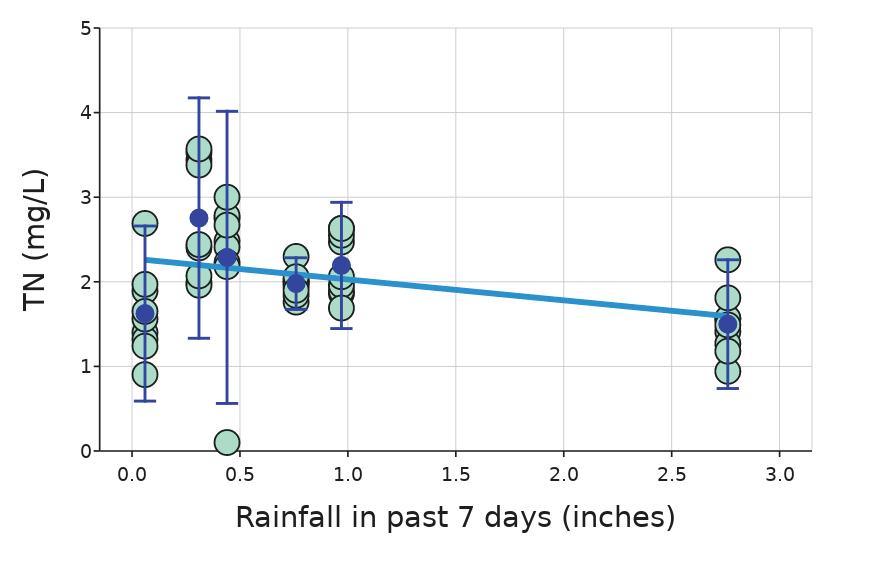
Figure 1. Graph of TN concentration in Elk River in relation to 7 day rainfall In Elk river only, linear regression analysis showed that increased weekly rainfall had a statistically significant relationship with a reduced concentration of TN (p < 0 05)
Effect of Rainfall on TP
TP was measured for each sample taken from Elk River and Mayhew creek, and total rainfall in the 3 days prior to sample collection as well as the 7 days prior to sample collection was calculated from data obtained from the Minnesota Department of Natural Resources Year to Date Precipitation Chart (Year to Date Precipitation Chart, n.d.). Data were analyzed by linear regression to determine whether there was a significant relationship between rainfall patterns and TP concentrations (Table 2) For the sites in Elk River, linear regression analysis showed a statistically significant relationship between increased 3-day rainfall and an increase in TP concentration (Figure 2)
Table 2. r2 and p-values for TP concentration in Mayhew Creek and Elk River in relation to 3-day and 7-day rainfall
7 day 0 000 0 98
3 day 0 113 0 01 Mayhew 7 day 0 0119 0 61
3 day 0.019 0.52
Elk and Mayhew 7 day 0 00322 0 60
3 day 0 0139 0 32
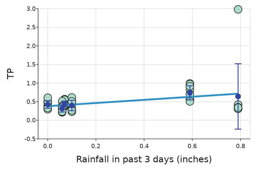
Figure 2. Graph of TP concentration in Elk River in relation to 3 day rainfall. In Elk river only, linear regression analysis showed that increased weekly rainfall had a statistically significant relationship with an increased concentration of TP (p < 0 05)
Effect of Rainfall on COD
COD was measured for each sample taken from Elk River and Mayhew Creek Data were analyzed by linear regression to determine whether there was a significant relationship between rainfall patterns and COD concentrations (Table 3) For the samples taken from both Elk River and Mayhew Creek, decreased COD concentrations had a statistically significant relationship with increased 3-day rainfall (Figure 3).
Table 3. r2 and p-values for COD levels in Mayhew Creek and Elk River in relation to 3-day and 7-day rainfall
Comparison to COD
River Period prior to sampling
Elk (8 sites)
Mayhew (4 sites)
Elk and Mayhew
7 day 0 0502 0 10
3 day 0 0211 0 29
7 day 0 00045 0 92
3 day 0.169 0.05
7 day 0 0249 0 19
3 day 0 0637 0 03
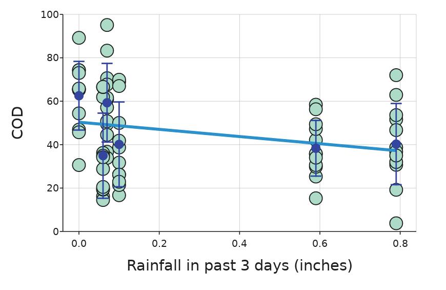
Figure 3. Graph of COD values in relation to 3-day rainfall for both Elk River and Mayhew Creek In both rivers, linear regression analysis showed a statistically significant relationship between decreased COD levels and increased 3-day rainfall levels (p < 0 05)
Effect of rainfall on E coli MPN
For each sample collected from Elk River and Mayhew Creek, a 100 mL of sample was used to measure total coliform and E coli counts For every sample, the total coliform count exceeded the upper limit of the test (2419.6 MPN/100 mL). Because of this, data for total coliform counts were not used. E. coli MPN counts were consistently within the test range, and these data were analyzed by linear regression to determine whether there was a significant relationship between 7-day or 3-day rainfall totals and E. coli counts. Analysis showed no significant
relationships between rainfall levels and E. coli counts for any river (Table 4).
Table 4. r2 and p-values for E coli MPN levels in Mayhew Creek and Elk River in relation to 3-day and 7-day rainfall.
River Period prior to sampling Comparison to MPN
Elk (8 sites)
Mayhew (4 sites)
Elk and Mayhew
7 day 0.0213 0.29
3 day 0 0161 0 36
7 day 0 0941 0 14
3 day 0 00814 0 67
7 day 0 00759 0 47
3 day 0.00873 0.43
Discussion
The work presented represents an analysis of water quality trends in two Minnesota rivers Over the course of the summer of 2024, I took samples from 8 sites along Elk River and 4 sites along Mayhew Creek These sites had been previously determined by the lab in collaboration with the MPCA for the purpose of assessing the general Elk River watershed area. I monitored the two rivers in the same watershed area over the course of two months, measuring TN, TP, E coli, and TSS I also collected data on rainfall Linear regression analysis showed a significant relationship between higher rainfall in the week before a sample was collected and a lowered amount in TN concentration in Elk River This indicates that a higher amount of rainfall in a week before sample collection leads to higher water levels, effectively diluting the concentration of nitrogen, without causing enough runoff of nitrogen to increase the nitrogen level. However, it does appear that there is a small increase in nitrogen levels with a small amount of rainfall, suggesting that a small amount of rainfall leads to runoff increasing TN levels, but past a small amount, increased rainfall only leads to higher water levels and
Charlo Vasicek
nitrogen runoff does not impact TN levels. Linear regression analysis also showed a significant relationship between higher amounts of rainfall in the three days before sample collection and an increase in TP levels in Elk River. This indicates that a higher amount of rainfall immediately before sample collection may lead to significant phosphorus runoff, which is then removed or diluted in rivers after a week, since there is no relationship between 7-day rainfall and higher TP
The data from Elk River and Mayhew Creek were initially collected with the intention of combining the data from both rivers to determine trends in water quality across the watershed area, and because of this, the sampling sites were not evenly distributed between Elk River and Mayhew Creek, with only 4 sites being sampled in Mayhew Creek and 8 being sampled in Elk River However, both of the trends found only applied significantly to one river, Elk River. Some trends came close to significance in Mayhew Creek, such as the relationship between COD and rainfall (p = 0 05) Throughout the study, it was observed that even sites very near each other in the same river would have very different measurements of COD, TN, TP, E. coli, and TSS. In addition, the fact that no significant trends extended to Mayhew Creek indicates that although Mayhew Creek and Elk River are very geographically close to each other, the factors impacting their water quality vary drastically.
The trends found in TN and TP concentrations can be used to predict when Elk River may be more safe for use, as well as help to determine sources of water quality impairment. Since increased TP was significantly correlated with increased 3 day rainfall, phosphorus content in Elk River may likely be coming from runoff sources such as fertilizer However, since increased 7 day rainfall was significantly correlated with decreased TN, nitrogen content may not be significantly increased by runoff, and the rainfall may only be effectively diluting nitrogen concentrations Although it has been observed that elevated levels of phosphorus can
stimulate growth of bacteria in sediment in lake environments, no trends were found between E. coli and TP concentrations No correlations were found between E coli and 3 day or 7 day rainfall, or nitrogen levels, so there is no evidence that E. coli concentrations were significantly increased by runoff from sources such as manure. Many spikes of very high E. coli concentrations were observed, and only one sample contained acceptable levels of E coli
Future Work
In the future, TSS will be measured using the updated procedure to gain accurate measurements of TSS in these rivers over time. In addition, tests such as microfluidic quantitative PCR will be performed to determine possible sources of bacterial contamination The data from these tests will help to track and determine more trends in factors affecting water quality in these rivers, as well as help to track specific sources of bacterial contamination, which will help efforts to improve water quality This work will contribute to a better understanding of Minnesota’s rivers, and this information will help people and wildlife to have access to cleaner and safer waters
Acknowledgements
I would like to thank Dr Kati Kragtorp for her advice and guidance which has made this project possible. I would also like to thank Dr. Satoshi Ishii, a professor in the Department of Soil, Water, and Climate at the University of Minnesota, who gave me the opportunity to work in the Ishii Lab this summer I am grateful to all of the members of the Ishii Lab who I worked with, and value the experiences and skills I learned through this project.
References
Alegbeleye, O O , & Sant’Ana, A S (2020) Manure-borne pathogens as an important source of water contamination: An update on the dynamics of pathogen survival/transport as well as practical risk mitigation strategies International Journal of Hygiene and Environmental Health, 227, 113524 https://doi org/10 1016/j ijheh 2020 113524
Bacteria | Minnesota Pollution Control Agency (n d ) Retrieved June 23, 2024, from https://www pca state mn us/pollutants-and-contaminants/bacteria
Mallin, M A , & Cahoon, L B (2020) The Hidden Impacts of Phosphorus Pollution to Streams and Rivers BioScience, 70(4), 315–329 https://doi org/10 1093/biosci/biaa001
Minnesota’s impaired waters list | Minnesota Pollution Control Agency (n d ) Retrieved June 22, 2024, from https://www pca state mn us/air-water-land-climate/minnesotas-im paired-waters-list
Rytkönen, A , Meriläinen, P , Valkama, K , Hokajärvi, A -M , Ruponen, J , Nummela, J , Mattila, H , Tulonen, T , Kivistö, R , & Pitkänen, T (2024) Scenario-based assessment of fecal pathogen sources affecting bathing water quality: Novel treatment options to reduce norovirus and Campylobacter infection risks Frontiers in Microbiology, 15, 1353798 https://doi org/10 3389/fmicb 2024 1353798
Vadde, K K , McCarthy, A J , Rong, R , & Sekar, R (2019) Quantification of Microbial Source Tracking and Pathogenic Bacterial Markers in Water and Sediments of Tiaoxi River (Taihu Watershed) Frontiers in Microbiology, 10, 699 https://doi org/10 3389/fmicb 2019 00699
Yang, X , Wu, X , Hao, H , & He, Z (2008) Mechanisms and assessment of water eutrophication Journal of Zhejiang University SCIENCE B, 9(3), 197–209 https://doi org/10 1631/jzus B0710626
Year to Date Precipitation Chart (n d ) Minnesota Department of Natural Resources Retrieved January 2, 2025, from https://www dnr state mn us/climate/climate monitor/precipcharts html