2 minute read
NBR


A. Training vs Validation Plots of the model The training samples and validation samples are in the ratio 7:3. The curves in Figure 5 and Figure 6 depicted how the training samples vary with the validation samples. The test is done 250 epochs. Early stopping decreased the computational cost by stopping the iteration early. So, we employed early stopping, we found that the accuracy is achieved in fewer epochs only. For our dataset, it is seen in the validation plot that the training loss and validation loss are gradually decreasing with increasing epochs and stabilize around a point. A little difference of 0.0376is observed which indicates a good fit and we can infer that the performance of the model is good on both the train and validation sets. Moreover, the difference between validation accuracy and training accuracy is also small and the curve increases w.r.t increase in the number of epochs and seems to stabilize around a point, indicating a good fit. We have used AUC (Area Under the Curve) ROC (Receiver Operating Characteristics) curve to evaluate the performance of the model. We also used different metrics like accuracy, precision, recall, f1-score, and kappa-coefficient to quantitivelyevaluatethe performance and prediction capability of the model. B. AUC and ROC curve AUC helps us to estimate the classification capability of a mode and ROC Curves explain the performance of the model. It plots a graph between the true positive rate (TPR) and false-positive rate (FPR) to predictive model. It uses separate probability thresholds. When AUC is higher, it reflects that the model is performing better in predicting false as false and true as true. The TPR is evaluated as shown in equation 6. It describes model prediction capabilityin predicting positive class as positive. TPR = Tp / (Tp + FN) (6)
The FPR is calculated from the ratio of false positive (Fp) with the sum of (Fp) and th e true negative (Tn) number given by equation 7. It helps to understand how frequently a positive class is predicted when the model output a negative class. FPR = 1 − Specificity = Fp/(Tn + Fp) (7)
Advertisement
The x-axis with a small value indicates lower Fp and higher Tn. The large values on the y-axis indicate lower FN and higher TP. We have also computed the micro-average and macro-average of the ROC curve and ROC area. The results for AOC and ROC curve are shown in Figure 7 and the zoomed version is shown in Figure 8.
C. Precision Precision is also known as a positive predicted value. It is calculated by dividing the number of TP by the sum of the TP and Fp shown in equation 8.
P recision = TP /(TP + Fp) (8)
D. Recall (sensivity) The recall is evaluated by dividing TP and the sum of the TP and the FN number shown in equation 9. It estimates the correctness of pixel detection of each category [44].
Recall = TP /(TP + FN ) (9)
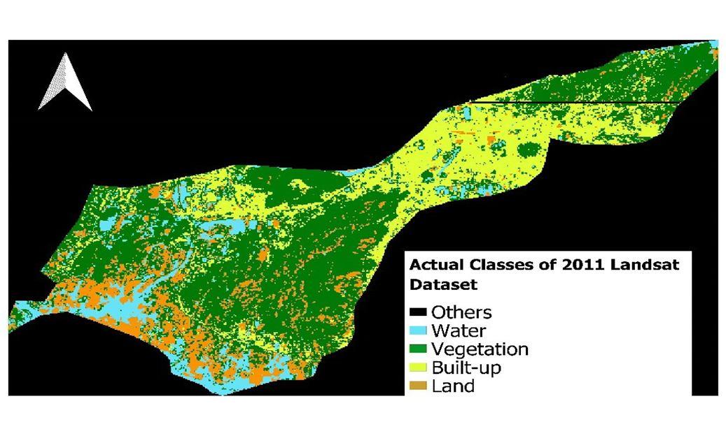
Fig. 3. Actual classification Map of Guwahati City